A Prediction Model of Hydrodynamic Landslide Evolution Process Based on Deep Learning Supported by Monitoring Big Data

Owing to the complex formation mechanism of hydrodynamic landslides and the involvement of multiple influencing factors, the accuracy of the current prediction model of hydrodynamic landslide evolution process is unsatisfactory. This limitation prevents adequate monitoring and early warning on possible landslides in an area. To improve the accuracy of prediction model of hydrodynamic landslide evolution process supported by monitoring big data, the variational mode decomposition (VMD) and support vector regression (SVR) based on deep learning were integrated in the present study. Typical hydrodynamic landslide in the Three Gorges Reservoir Area (TGRA) in China is used as a case study for landslide displacement prediction. First, the VMD was utilized to decompose the cumulative displacement into the trend, periodic, and random terms. Then, external factors were decomposed into subsequences, and those characterized by periodicity and randomness were selected as input datasets. The associated displacement terms were then predicted using the Random Search–Support Vector Regression model. Finally, the total displacement was obtained by superimposing the three predicted components, and this was used to evaluate the performance of the model. The results show that the model improves the performance and accuracy of predicting the displacement associated with a hydrodynamic landslide, and the relative error is ≤2%.

Introduction

A landslide is a geological hazard associated with severe environmental consequences, and it often occurs in China. The prediction of landslide deformation is an established approach for preventing landslide hazards (Tien et al., 2018). Hydrodynamic landslides commonly occur in reservoir areas, and their displacement curves exhibit stages associated with the rainfall and reservoir level changes. These changes and other influencing factors (Huang, 2007; Xu et al., 2008) in the reservoir area manifest after years. Therefore, accurate prediction of landslide displacement is challenging, and thus, this remains an area of significant interest in the field of natural disaster prevention and control.

Following the impoundment of the Three Gorges Reservoir in China in 2009, disasters involving hydrodynamic landslides have occurred frequently in the Three Gorges Reservoir Area (TGRA). These landslides, which have caused tremendous losses, are attributed to changes in the reservoir water level, rainfall, and other factors. Therefore, several studies on the prediction of landslides and the associated damage are available. Studies on landslide displacement prediction can roughly be partitioned based on the duration and prediction method into three groups (Xu et al., 2011). The empirical approach involving the landslide displacement rate was used to generate initial prediction models, which were then improved by comparing the modeled to field monitoring data (Sidle et al., 1985). The statistical approach models, such as the Verhulst (Long et al., 2008), Verhulst inverse function (Belle et al., 2014), golden section, Markov chain prediction (Zhao et al., 2013), and time-series (Mazzanti et al., 2011) then improved landslide deformation prediction. Further, the intelligent analysis and prediction approach, which emerged in the 1990s, involves artificial intelligence-based nonlinear theories, which produce data-driven models for systematic prediction of landslide deformation (Korup and Stolle, 2014).

However, models produced using existing landslide displacement prediction methods are based mainly on geological monitoring data (e.g., reservoir water level, rainfall, and landslide displacement) to predict future displacement (Zhang et al., 2015). Models including the Gray (GM) (Huang et al., 2017), extreme learning machine (ELM) (Bernardie et al., 2014), and support vector machine (SVM) (Lian et al., 2014) involve different neural networks (Bergstra and Bengio, 2012; Hochreiter and Schmidhuber, 1997) (e.g., back propagation (BPNN), recurrent (RNN), etc.) and have generated varying prediction results. In fact, different models are associated with advantages and drawbacks. The GM, for example, involves a simple structure but the prediction accuracy is unsatisfactory, while the ELM is fast and requires little training data, and the BPNN commonly produces an unsatisfactory fitting performance for complex nonlinear curves.

The support vector regression (SVR) model is based on the machine learning theory, and it involves few training samples and a simple structure. Its prediction performance is better than that of a conventional neural network model, and thus, it is suitable for landslide displacement prediction involving a short monitoring period. SVR parameter search methods include the following: particle swarm optimization (PSO), genetic algorithm (GA), grid search (GS), and random search (RS). The GA and PSO are heuristic algorithms involving complex operations, while the GS algorithm encompasses all possible solutions for a given parameter range, and thus, it exhibits a higher classification accuracy. Compared to other methods, the RS algorithm is associated with a comparable prediction performance and it is computationally inexpensive (Wen et al., 2017).

The evolution of landslide displacement is influenced by many factors involving complex relationships that are difficult to characterize accurately. Therefore, in data-driven multivariate prediction models, time series decomposition methods are commonly introduced to simplify the problem (Xu et al., 2011). The displacement time series is decomposed into parts associated with varying data characteristics such as, the trend, periodic, and random terms, and varied models serve in forecasting the decomposition terms. The prediction accuracy of a model increases as the factors considered are increased. The moving average method (Huang et al., 1998; Xu et al., 2011) and the empirical mode decomposition (EMD) (Liu et al., 2020) are methods commonly employed for decomposition in hydrodynamic landslide displacement prediction studies that produce satisfactory results. However, controlling the decomposition terms obtained by these methods is challenging, and therefore, correlations between different factors and the displacement decomposition terms are poor. In addition, the physical meaning of each decomposition term is inadequately explained using these methods (Dragomiretskiy and Zosso, 2014). The variational mode decomposition (VMD) method (Wang and Min, 2014) employed in the present study resolves these shortcomings. Similar to the EMD, the VMD is a signal processing method suitable for handling non-smooth and non-linear signals. It was recently applied at the displacement decomposition stage of landslide deformation prediction (Dragomiretskiy and Zosso, 2014) and produced good results.

In the present study, the Bazimen landslide, which occurred in the TGRA, was used as a case study to establish a hydrodynamic landslide displacement prediction model by integrating the VMD and RS–SVR methods. In the time series model, the VMD method was used to decompose the cumulative monitored displacement into the trend, periodic, and random terms, thereby assigning a clear physical meaning to each decomposition term. After determining factors strongly correlated to each term, the RS–SVR method was utilized to predict the landslide displacement. The prediction results were then compared with those for the KRR, ELM, LSTM, and GS–SVR models.

Methodology

Time Series Analysis

In general, according to the additive time series, the cumulative displacement of a landslide can be expressed as follows:

$X\left(t\right)=\varphi \left(t\right)+\eta \left(t\right)+\epsilon \left(t\right)(1)$

where $X\left(t\right)$ denotes the time series displacement value, $\varphi \left(t\right)$ represents the trend term displacement function, $\eta \left(t\right)$ is the periodic term displacement function, and $\epsilon \left(t\right)$ designates the random term displacement function involving uncertainty. Landslide deformation is mainly controlled by intrinsic (topography, geological structure, etc.) and external (temperature, rainfall, reservoir level, etc.) factors (Li and Xu, 2003). The trend term displacement associated with intrinsic factors is an approximate function that increases monotonically with time. It reflects the overall landslide cumulative displacement. Conversely, the periodic term displacement is an approximate function controlled by factors such as, rainfall, reservoir level change, etc. Unpredictable episodic factors including human activities and seismic effects also influence the evolution of landslide displacement, and this is expressed as the random term displacement (Vapnik, 1995; Zheng et al., 2005).

Variational Mode Decomposition

VMD is an adaptive non-recursive approach for mode variation and signal processing. The technique is advantageous because the mode decompositions can be determined. Its adaptiveness is demonstrated by evaluating mode decompositions associated with a given sequence according to the actual situation. The subsequent search and solution steps can be adaptively matched to the optimal central frequency and the finite bandwidth of each mode. Consequently, effective separation of the intrinsic mode component (IMF), frequency domain partitioning of the signal, and the N-efficient decomposition components of a given signal can be achieved. This approach is suitable for finding the optimal solution of a variational problem because it overcomes the endpoint effect and mode component mixing issues associated with the EMD method. In addition, it involves a better mathematical foundation suitable for reducing the complexity and nonlinearity of time series non-stationarity, decomposition into relatively smooth sub-series involving different frequency scales, and handling of non-stationary sequences. In fact, the basis of the VMD is to formulate and solve variational problems.

First, the variational problem is formulated by assuming that the original signal f can be decomposed into k components, and the decomposed sequence is guaranteed to represent a finite bandwidth mode component characterized by a central frequency. The sum of the estimated bandwidths of each mode is minimized, with the sum of all modes equaling the monitored signal as the constraint. The constrained variational problem is then expressed as follows:

$\begin{array}{l}\underset{\left\{u_k\right\},\left\{{\omega }_k\right\}}{\min }\left\{{\displaystyle \sum _k{\Vert \left[{\partial }_t\left[\left(\delta \left(t\right)+j/\pi t\right)\ast u_k\left(t\right)\right]e^{-j{\omega }_{k}t}\right]\Vert }_2^2}\right\}\\ s.t.{\displaystyle \sum _{k=1}^K{u}_k=f}\end{array}(2)$

where K represents the modes requiring decomposition (positive integer), $\left\{u_k\right\},\left\{{\omega }_k\right\}$ denote the central frequency of the kth mode component after decomposition, $\delta \left(t\right)$ is the Dirac function, and $\ast$ designates the convolution operator.

Equation 2 is then solved, and the Lagrange multiplier λ is used to convert the constrained variational problem into an unconstrained variational problem. The generalized Lagrange expression obtained is given as follows:

$\begin{array}{l}L\left(\left\{u_k\right\},\left\{{\omega }_k\right\},\lambda \right)=\alpha {\displaystyle \sum _k{\Vert [{\partial }_t\left[\left(\delta \left(t\right)+\raisebox{1ex}{$j$}\!\left/ \!\raisebox{-1ex}{$\pi t$}\right.\right)\ast u_k\left(t\right)\right]e^{-j{\omega }_{k}t}\Vert }_2^2}+\\ {\Vert f\left(t\right)-{\displaystyle \sum _k{u}_k\left(t\right)}\Vert }_2^2+\langle \lambda \left(t\right),f\left(t\right)-{\displaystyle \sum _k{u}_k\left(t\right)}\rangle \end{array}(3)$

where α is a quadratic penalty factor which reduces the Gaussian noise interference. The alternating directional multiplier (ADM) iterative algorithm combined with the Parseval-Plancheral theorem and Fourier isometric transforms were employed for optimization to obtain each mode component and the central frequency. The saddle point of the extended Lagrange function was then sought by iterations involving $u_k$, ${\omega }_k$, and $\lambda$. The detailed process involved the following equations:

${\widehat{u}}_k^{n+1}\left(w\right)\leftarrow \frac{\widehat{f}\left(w\right)-\underset{i\ne k}{{\displaystyle \Sigma }}{\widehat{u}}_i\left(\omega \right)+\widehat{\lambda }\left(\omega \right)/2}{1+2\alpha {\left(\omega -{\omega }_k\right)}^2}(4)$

${\omega }_k^{n+1}\leftarrow \frac{{\displaystyle {\int }_0^{\infty }\omega {\left|{\widehat{u}}_k^{n+1}\left(\omega \right)\right|}^{2}d\omega }}{{\displaystyle {\int }_0^{\infty }{\left|{\widehat{u}}_k^{n+1}\left(\omega \right)\right|}^{2}d\omega }}(5)$

${\widehat{\lambda }}^{n+1}\left(\omega \right)\leftarrow {\widehat{\lambda }}^n\left(\omega \right)+\gamma \left(\widehat{f}\left(\omega \right)-{\displaystyle \sum _k{\widehat{u}}_k^{n+1}\left(\omega \right)}\right)(6)$

where γ is the noise tolerance, which satisfies the fidelity requirement of signal decomposition, and ${\widehat{u}}_k^{n+1}\left(\omega \right)$, ${\widehat{u}}_i\left(\omega \right)$, $\widehat{f}\left(\omega \right)$, and $\widehat{\lambda }\left(\omega \right)$ are the Fourier transforms of ${\widehat{u}}_k^{n+1}\left(t\right)$, $f\left(t\right)$, and $\lambda \left(t\right)$, respectively.

The iterative solution process of VMD is summarized as follows:

S1: initialize ${\widehat{u}}_k^1,{\omega }_k^1,{\lambda }^1$ and maximize the iterations N, $n\leftarrow 0$.

S2: update ${\widehat{u}}_k$ and ${\omega }_k$ using Eqs. 4, 5.

S3: update $\widehat{\lambda }$ using Eq. 6

S4: If the accuracy convergence criterion is $\underset{k}{{\displaystyle \Sigma }}{\Vert {\widehat{u}}_k^{n+1}-{\widehat{u}}_k^n\Vert }_2^2/{\Vert {\widehat{u}}_k^n\Vert }_2^2<\epsilon$ and $n<N$ is not satisfied, then return to the second step, otherwise complete the iteration and obtain the final ${\widehat{u}}_k$ and ${\omega }_k$.

Support Vector Regression

The SVR model proposed by Vapnik (1995) has been widely used for solving nonlinear problems. In this model, the sample data is divided into training and test samples. Then, the pre-selected input vector (training samples) is mapped to a high-dimensional feature space. The best fit is then obtained in the space of optimal decision function models and the testing samples are utilized to validate the results. This approach is primarily intended for predictive analysis (Üstün et al., 2005; Wang et al., 2004; Yilmaz, 2010). Coordinates {$x_j$, $y_j$} are the feature vectors of the sample data, where $x_j =\left\{x_{j1},x_{j2},\cdots ,x_{jp}\right\}$ is the factor controlling $y_j$ and p is the number of values in $y_j$. The regression estimation function of the support vector machine (SVM) is expressed as follows:

$f\left(x\right)=W^T\varnothing \left(x\right)+b(7)$

where $\varnothing \left(x\right)$ is the nonlinear mapping function of the sample data, which is mapped to the feature space, $W^T$ represents the autocovariance coefficient of the estimation function, and b is the bias of the estimation function. The parameters $W^T$ and b can be obtained by minimizing the following equation:

$D\left(f\right)=\frac{1}{2}\Vert W^2\Vert +\frac{C}{n}{\displaystyle \sum }_{j=1}^n{R}_{\epsilon }\left[y_j,f\left(x_j\right)\right](8)$

where $D\left(f\right)$ is a generalized optimal classification plane function, which considers the minimum number of incorrect sample points and the maximum classification interval, $W^2$ represents the complexity of the model, C designates the penalty parameter, and $R_{\epsilon }$ denotes the error control function of $\text{ε}$. Thus, the optimization problem can be expressed as follows:

$\text{minQ}\left(\text{W},\text{ξ}\right)=\frac{1}{2}\Vert W^2\Vert +C{\displaystyle \sum }_{j=1}^n{\xi }_j+{\xi }_j^{\text{*}}(9)$

$W^T\varnothing \left(x_j\right)+b-y_j\le \epsilon +{\xi }_j(10)$

$y_j-W^T\varnothing \left(x_j\right)-b\le \epsilon +{\xi }_j^{\text{*}}(11)$

${\xi }_j\ge 0,{\xi }_j^{\text{*}}\ge 0\left(j=\mathrm{1,2},\cdots ,n\right)(12)$

where ${\xi }_j$, ${\xi }_j^{\text{*}}$ are relaxation factors.

If partial derivatives of W, b, and ${\xi }_j$ are 0, then, based on the Lagrange equation and duality theory, the double optimization problem can be expressed as follows:

$\text{L}\left(\text{W,a,b,}\epsilon \text{,y}\right)=\text{min}\frac{1}{2}{\displaystyle \sum }_{r,j=1}^n{\left(a_r-a_r^{\ast }\right)}^T{H}_{r,j^{\text{*}}}(13)$

$\left(a_r-a_r^{\text{*}}\right)+\epsilon {\displaystyle \sum }_{r,j=1}^n\left(a_r-a_r^{\text{*}}\right)+{\displaystyle \sum }_{r=1}^n{y}_r\left(a_r-a_r^{\text{*}}\right)(14)$

${\displaystyle \sum }_{r=1}^n\left(a_r-a_r^{\text{*}}\right)=0,\left(0\le a_r,a_r^{\ast }\le C\right)(15)$

$H_{r,j}=K\left(x_r,x_j\right)=\varnothing {\left(x_r\right)}^T\varnothing \left(x_j\right),\left(r=\mathrm{1,2},\cdots ,n\right)(16)$

Here, $K\left(x_r,x_j\right)$ is the kernel function, which in the present study is a Gaussian kernel function (RBF). Thus, the SVR model can be expressed as follows:

$f\left(x\right)={\displaystyle \sum }_{j=1}^n\left(a_j^{\text{*}}-a_j\right)K\left(x_j,x\right)+b(17)$

Linear problems in engineering can be solved using the inseparable SVM. Based on a mapping function, the linearly inseparable problem is mapped to a linearly separable problem in a high-dimensional space. This model, which is based on the statistical learning theory requires few samples for learning. Thus, it performs better than conventional feedback (BP) neural networks because of its simple structure. Therefore, this model is suitable for predicting landslide displacement involving a short monitoring period.

Case study:Bazimen Landslide

Data Source and Description

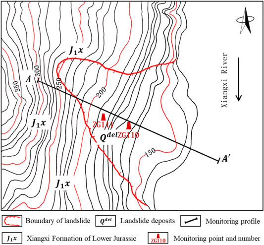
The Bazimen landslide is located on the right bank of the Xiangxi River in TGRA, as shown in Figure 1, with the following geographical coordinates: longitude 110°45′30″, latitude 30°58′16″. The slope is oriented north-south, the landslide is spread in a winnowing fan shape at the foot of the slope, in the range of 139～280m in elevation, high in the west and low in the east, sloping to the east, and the ground slope of the landslide is 10–30°, which is ladder-like and undulating. The part of the landslide above the water surface is 380 m long, 100–500 m wide, 10–35 m thick, and has a volume of about two million cubic meters.

FIGURE 1

FIGURE 1. Illustration of the monitoring layout in the Bazimen landslide area.

Ten deformation monitoring points are present across the landslide area, and the oldest points (ZG110 and ZG111) are in the area associated with the largest landslide deformation. These representative points adequately reflect the evolution trend of the displacement linked to the Bazimen landslide. In the present study, the monitoring data from the ZG110 point was utilized. According to the data, the landslide deformation rate increased annually from May to September, and the cumulative displacement curve is steeper in this interval, as shown in Figure 2. As of December 31, 2018, the cumulative horizontal displacement and cumulative displacement direction of the ZG110 monitoring point were 1,525.73 mm and 117°, respectively.

FIGURE 2

FIGURE 2. Relationship between the cumulative displacement, reservoir water level, and rainfall in the Bazimen landslide area.

The TGRA is characterized by an intense rainy season, and the average annual rainfall exceeds 1,000 mm. Rainfall, which significantly impacts the evolution of the landslide deformation in the TGRA, exhibits an obvious periodicity, which reflects the rainy and dry seasons (Figure 2). In the TGRA, rainfall is mainly concentrated between May–September, and the maximum monthly rainfall commonly exceeds 220 mm, with an average of 321.3 mm during the monitoring period. Considering that the Three Gorges Hydropower Station has been operational since 2009, in the present study, the reservoir water level dispatch data from 2009 to 2018 were utilized. Owing to flood control and water storage requirements, the reservoir water level change data, which involve a maximum variation of 30 m, exhibit obvious cyclical characteristics. Considering a cycle from October 2016 to October 2017 as an example, the reservoir water level rose from November to May, and stayed high during operation in June, and then decreased from July to September (Figure 2).

Prediction of Landslide Evolution Process Supported by Monitoring Big Data

In the present study, monitoring data for the ZG110 point from January 2009 to December 2018 were used to assess the suitability of our model. Monitoring data for the first 100 months served as the training samples, while data for the next 20 months were used as the testing samples. To minimize the impact of missing data or information in the displacement decomposition and model training, and to enhance learning of the monitoring data during the entire process by the prediction model, the sequence “displacement decomposition → partitioning of the dataset into training and testing samples” was not pursued. In contrast, the approach used involved “dividing the dataset into training and testing samples → displacement decomposition”. Finally, indicators, such as the absolute error (AR), relative error (RE), and root mean square error (RMSE), were used to evaluate the prediction performance of the model, and the entire process is illustrated in Figure 3.

FIGURE 3

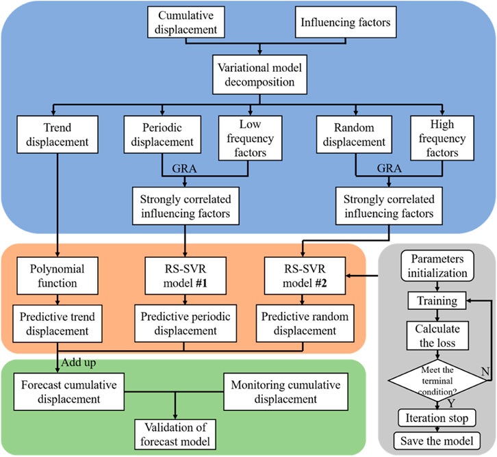
FIGURE 3. Flowchart of the components utilized for landslide displacement prediction. Decomposition of the cumulative displacement and the controlling factors.

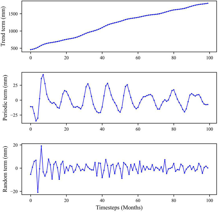
The VMD model was used to decompose the cumulative displacement associated with the Bazimen landslide into the trend, periodic, and random terms (Figure 4). The IMF parameter K in the VMD model, α, the tolerance of the convergence criterion τ, and the time step were set to 3, 1, 10⁻⁶, and 0.01, respectively. In the model decomposition results, the low-frequency component corresponds to the displacement of the periodic term, while the high-frequency component represents the displacement of the random term, and the residual component is the displacement of the trend term.

FIGURE 4

FIGURE 4. Plot showing the decomposition of the cumulative displacement.

Infiltration of rainfall alters the physical and mechanical properties of the landslide mass, and this increases the water content and bulk weight of the slope mass. Besides, infiltration also changes the shear strength, sliding force, and slip resistance of the slope mass because of effects of the static and dynamic water pressures. These impacts are prominent during long-term or intense rainfall, which significantly affects the stability of the landslide mass.

Scouring of the landslide mass associated with rainfall also affects the slope stability. Intense rainfall produces slope runoff, which promotes scouring of the surface of the landslide mass and erosion of its base, and this ultimately, changes the structure of the landslide mass. The resulting increase in the area and mass of the landslide prolapse severely affect the stability of the landslide mass. Concurrently, rainfall can easily penetrate the slip zone through fractures produced by the landslide area deformation. This significantly reduces the strength of the slip zone and further weakens the stability of the landslide area. To assess the impact of long-term rainfall, the rainfall of a month (R1) and that of the chosen and previous month (R2) were selected as the main factors controlling the landslide deformation.

The physical and mechanical properties of the slope mass within the influence of the reservoir water level are also affected because the landslide area soil mass comprises mainly siltstones and sandstones. Therefore, the shear strength of the soil mass beneath the water level is significantly decreased. Simultaneously, the scouring caused by the rise and decline of the reservoir water alters the morphology of the slope angle and landslide mass, which is detrimental to the stability of the landslide mass.

The mechanical impact of the reservoir water level change on the landslide mass is mainly associated with hydrostatic and dynamic water pressures. The hydrostatic pressure acts vertically on the landslide mass, which enhances the stability of the landslide area. However, the submerged soil particles also experience buoyancy simultaneously, which reduces the stability of the slope mass. The dynamic action mainly involves the force generated by groundwater in pores between soil particles in the slope mass. The central gentle section of the Bazimen landslide area is mostly beneath the 145 m level because of the rapid reservoir water level decline and the low permeability of the landslide mass. Therefore, the groundwater level in the slope mass lags the reservoir water level decline, and this produces a positive drop in the reservoir water level. Thus, groundwater seeps from the landslide mass, and the infiltration pressure is directed towards the exterior of the slope mass, thereby significantly deforming the slope mass during the sudden reservoir water level decline. Considering that the impact of the reservoir water level fluctuation is a slow process, changes in a month (W1) and 2 months (W2) were considered controlling factors. The increase of the landslide displacement in a month (D1) and the cumulative increment for 2 months (D2) were also selected as influencing factors.

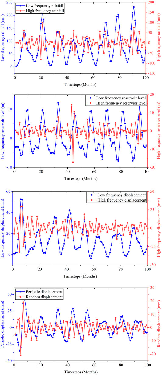
If the IMF parameter K is set to two in the VMD model, each influencing factor is decomposed into a high-frequency and a low-frequency term, while other parameters in the model are unchanged. Decomposition results associated with the rainfall (R1), the reservoir level change (W1), and the incremental displacement (D1) in a month as well as the cumulative landslide displacement are displayed in Figure 5. The dotted lines in blue represent the low-frequency terms of each indicator, and these are characterized by steady cyclical variations. The eight peaks and troughs associated with the indicator curve for each influencing factor correspond to the eight monitoring periods of the selected training dataset. Similarly, the dotted lines in red depict the high-frequency term of various indicators, and the curves exhibit irregular variation during the monitoring period. Therefore, the high-frequency term is suitable for predicting the random displacement, while the low-frequency term is useful for forecasting the periodic displacement.

FIGURE 5

FIGURE 5. Plots exhibiting the decomposition of different influencing factors.

Based on GRA method, the grey correlation degree ${\gamma }_k$ between the periodic displacement, the random displacement, and the controlling factor decomposition terms were calculated and the results are presented in Table 1. A ${\gamma }_{k }$ value >0.6 between the displacement decomposition term and the decomposition term of a controlling factor indicates that they are closely related (Schölkopf, 2008) and validates the rationale for utilizing the chosen factors as the prediction model input.

TABLE 1

TABLE 1. GRA results between the displacement periodic and random terms and the influencing factors.

In this study, the amount of discrete data used for fitting is small, the curve shape is smooth, and complex fitting methods are not required. The ideal effect can be achieved by using cubic polynomial fitting. First, fitting of the trend term was achieved using the following least squares-based polynomial:

$\text{ε}\left(\text{t}\right)=\text{a}{t}^3+b{t}^2+ct+d(18)$

The calculated data for various parameters are presented in Table 2, and the best-fit curve based on the cubic polynomial least squares method was obtained. The main purpose of the least squares curve-fitting is to generate the minimum sum of squares for each error, and the prediction results are shown in Figure 6.

TABLE 2

TABLE 2. Data for displacement trend parameters associated with the polynomial fitting.

FIGURE 6

FIGURE 6. Plot showing the prediction of the trend displacement.

Periodic Displacement Prediction

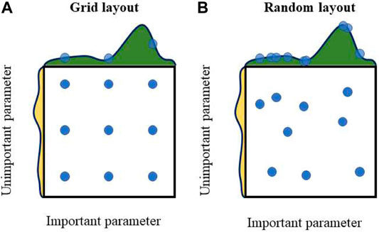
The periodic displacement reflects the influence of external factors, such as rainfall and the reservoir water level on the landslide displacement. In the present study, the RS–SVR model was employed for prediction of the periodic displacement. RS algorithm is a simple direct method used to find the best parameter set of an SVR model. The parameters C and γ in the model are independent, and thus, the optimal-parameter-searching process can be performed simultaneously after selecting sets of values for both parameters. Each pair of γ and C values is then evaluated through cross-validation, and that with the highest accuracy is considered the optimal solution. In RS algorithm, the parameter-search process is random, where each parameter setting value is sampled from a distribution to obtain the possible value. The following are the advantages of the RS relative to the GS: the freedom to choose a budget independent of the number of parameters and possible values and the negligible effect on the efficiency because of the addition of parameters with no effect on the performance. Bergstra and Bengio empirically and theoretically demonstrated the superiority of the RS relative to the GS. The performance of the RS and GS for identical searches are shown in Figure 7.

FIGURE 7

FIGURE 7. Illustration of the (A) grid and (B) random search layouts.

According to existing studies, when using SVM algorithms for training and classification of datasets, the choice of parameters, such as the kernel and penalty factors significantly impact the accuracy and performance of the prediction model (Schölkopf, 2008). Therefore, reasonable model parameters can enhance the prediction accuracy and significantly elevate the efficiency of the model. The PSO (Eberhart and Kennady, 2002), GA (Chen et al., 2004), RS, and GS (Kennedy and Eberhart, 2002) are the most commonly used SVM parameter search methods. However, the parameter optimizations associated with the GA and PSO are characterized by randomness and chance, and thus, the optimal parameters determined may be local. Therefore, these algorithms classified as heuristic involve shortcomings. Conversely, the RS algorithm explores all possible solutions within a particular range, thereby yielding a more accurate final parameter selection.

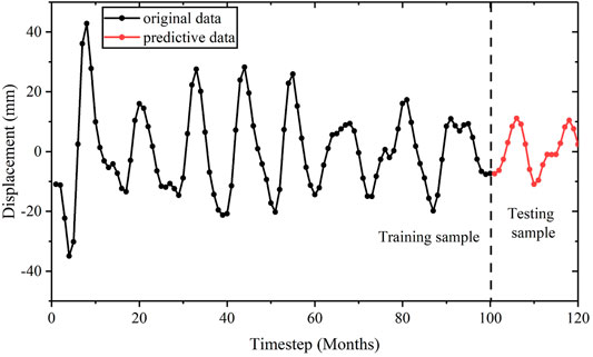
In the training phase of the model, the low-frequency components of the selected influencing factors associated with a timestep t served as the input. The optimal model parameters generated by the RS algorithm are presented in Table 3, while the training and validation data for the periodic term displacement are displayed in Figure 8. Obviously, the smooth curves of the prediction data exhibit periodic variation, which demonstrates the excellent performance of the RS-SVR prediction model.

TABLE 3

TABLE 3. Data for parameters of the GS-SVR model used for periodic displacement prediction.

FIGURE 8

FIGURE 8. Plot displaying the prediction of periodic displacement.

Random Displacement Prediction

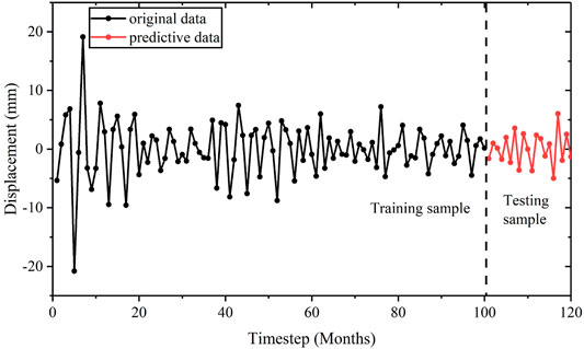
The random term displacement highlights the influence of uncertainty factors (e.g., human activities, earthquakes, etc.) on the change in landslide displacement. The displacement curve is characterized by obvious fluctuations. However, the RS-SVR model also displays excellent fitting and prediction performance for such data. In the training phase of the model, high-frequency components of controlling factors with a timestep t served as the input. Optimal parameters obtained using the RS algorithm are presented in Table 4, while the training and validation data of the random term displacement are shown in Figure 9. The smooth curves of the prediction data evidently display periodic variation, which also demonstrates the excellent performance of the RS-SVR prediction model.

TABLE 4

TABLE 4. Data for parameters of RS-SVR model used for the random displacement prediction.

FIGURE 9

FIGURE 9. Plot highlighting the prediction of random displacement.

Cumulative Displacement Prediction

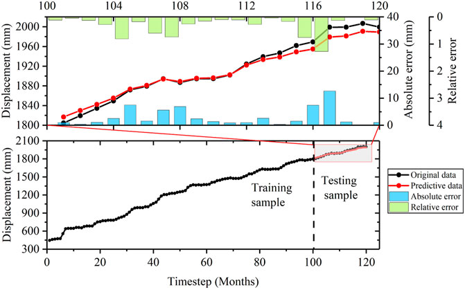
From Eq. 1, the cumulative displacement of the landslide was obtained through the linear summation of the trend, periodic, and random terms, and the prediction results are shown in Figure 10. The AE of the accumulated displacement associated with the Bazimen landslide displacement monitoring point ZG110 is less than 20 mm, while the RE is less than 2.0% for each month of the prediction duration. The prediction results demonstrate that the RS-SVR prediction model is consistent with the monitoring data. The predicted cumulative displacement also exhibits the step-like variation associated with the displacement monitoring curve. Therefore, the RS-SVR model adequately predicts the landslide displacement.

FIGURE 10

FIGURE 10. Plots highlighting the prediction of the cumulative displacement.

Evaluation and Comparison of Prediction Results

To demonstrate the superiority of the RS-SVR compared to other algorithms, the prediction results were compared with those of the KRR, ELM, LSTM and GS-SVR models. Monitoring data for the Bazimen landslide periodic displacement were utilized as the validation dataset, and the results are shown in Figure 11. Relative to the other four models, the RS-SVR (dotted lines in red) produced a better fit of the monitored periodic displacement and a superior performance. The RMSE values for the RS-SVR, GS-SVR, ELM, LSTM, and KRR models presented in Table 5 are 4.3950, 10.3673, 81.5314, 121.8, and 12.8, respectively. The values of 81.5314, 121.8974 and 88.4979 fully accommodate the prediction performance of each model.

FIGURE 11

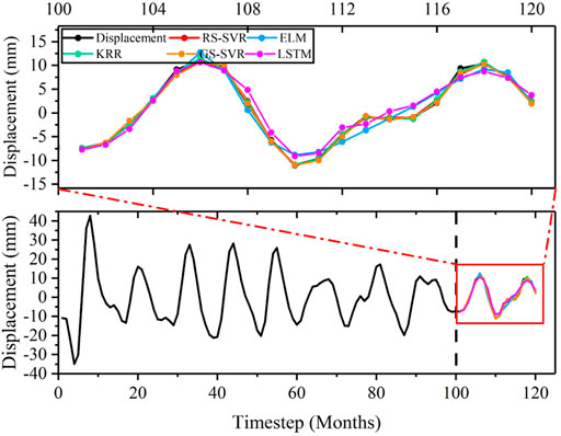
FIGURE 11. Plots showing a comparison of prediction accuracy of the periodic displacement for multiple models

TABLE 5

TABLE 5. RMSE data obtained for different prediction models.

However, this model also has applicable conditions and the biggest difficulty in the application of the new prediction model of landslide are: when the data size is insufficient, there is a chance of overfitting, resulting in a decrease in prediction accuracy; in addition, due to the small training data set, the model may not be able to learn all the features of the original data set. When using the new data set as the model input, the prediction accuracy of existing models will also decrease.

Conclusion

In the present study, the variational mode decomposition and random search-support vector regression algorithms were integrated to predict landslide displacement, and the results were validated using monitoring data for the Bazimen landslide. The findings of the study are summarized as follows:

1) VMD method has the advantage that the number of mode decompositions can be determined, and its adaptiveness is demonstrated by determining the number of mode decompositions of the given sequence according to the actual situation. And the VMD model can reasonably explain the physical meaning of each decomposition item: the monotonically increasing term is the periodic displacement, the high-frequency term is the random displacement, and the low-frequency term is the periodic displacement.

2) The model is based on statistical learning theory and has many advantages. Particularly, it requires only a very small sample for learning, has a simple statistical structure, and performs better than traditional backpropagation neural networks. Thus, the model is appropriate for predicting the displacement of landslides with only short-period observational data.

3) The results confirmed the decomposition of landslide displacement based on the VMD theory into the trend, periodic, and random terms, with each term associated to a distinct physical meaning. The cumulative displacement predicted represented the sum of predicted results for various decomposition terms. This approach produced a high decomposition efficiency and clear results, which validated its applicability in engineering.

4) Based on the cumulative displacement of the landslide and the influencing factors obtained using the VMD method, three decomposition terms associated with the displacement were predicted. The displacement prediction results obtained from the periodic and random terms demonstrated an outstanding prediction performance using the RS-SVR model, and the displacement prediction error was <2%.

5) The prediction accuracy of the RS-SVR model exceeded those of the GS-SVR, ELM, LSTM, and KRR models. Therefore, in the displacement prediction of hydrodynamic landslides, the RS-SVR model exhibits broad application prospects.

Data Availability Statement

The original contributions presented in the study are included in the article/Supplementary Material, further inquiries can be directed to the corresponding author.

Author Contributions

Contribution of KZ is the prediction of landslide evolution process supported by monitoring big data. The contribution of JQ is the trend displacement prediction. The contribution of WX is the critical revision of the manuscript for important intellectual content. The contribution of YL is the cumulative displacement prediction. The contribution of HH is the monitoring data analysis of Bazimen Landslide.

Funding

This work is supported by the National Natural Science Foundation of China (No.51939004), the Fundamental Research Funds for the Central Universities (No. B200204008), the Open Foundation of National Field Observation and Research Station of Landslides in the TGRA of Yangtze River, China Three Gorges University (2018KTL03). We thank the National Field Observation and Research Station of Landslides in the TGRA of Yangtze River for their help in providing monitoring data for this study.

Conflict of Interest

The authors declare that the research was conducted in the absence of any commercial or financial relationships that could be construed as a potential conflict of interest.

Publisher’s Note

All claims expressed in this article are solely those of the authors and do not necessarily represent those of their affiliated organizations, or those of the publisher, the editors and the reviewers. Any product that may be evaluated in this article, or claim that may be made by its manufacturer, is not guaranteed or endorsed by the publisher.

References

Anonymous, R. C., Pearce, A. J., and O'Loughlin, C. L. (1985). Hillslope Stability and Land Use. Eos Trans. AGU 66 (44), 740. doi:10.1029/EO066i044p00740

CrossRef Full Text | Google Scholar

Belle, P., Aunay, B., Bernardie, S., Grandjean, G., Ladouche, B., Mazué, R., et al. (2014). The Application of an Innovative Inverse Model for Understanding and Predicting Landslide Movements (Salazie Cirque Landslides, Reunion Island). Landslides 11 (3), 343–355. doi:10.1007/s10346-013-0393-5

CrossRef Full Text | Google Scholar

Bergstra, J., and Bengio, Y. (2012). Random Search for Hyper-Parameter Optimization. J. Mach. Learn. Res. 13 (1), 281–305. doi:10.1016/j.chemolab.2011.12.002

CrossRef Full Text | Google Scholar

Bernardie, S., Desramaut, N., Malet, J.-P., Gourlay, M., and Grandjean, G. (2014). Prediction of Changes in Landslide Rates Induced by Rainfall. Landslides 12 (3), 481–494. doi:10.1007/s10346-014-0495-8

CrossRef Full Text | Google Scholar

Chen, P. W., Wang, J. Y., and Lee, H. M. (2004). “Model Selection of SVMs Using GA Approach,” in Paper presented at the IEEE International Joint Conference on Neural Networks, Budapest, Hungary, 25-29 July 2004 (IEEE).

Google Scholar

Dragomiretskiy, K., and Zosso, D. (2014). Variational Mode Decomposition. IEEE Trans. Signal. Process. 62 (3), 531–544. doi:10.1109/tsp.2013.2288675

CrossRef Full Text | Google Scholar

Eberhart, R., and Kennedy, J. (2002). “A New Optimizer Using Particle Swarm Theory,” in Paper presented at the Mhs95 Sixth International Symposium on Micro Machine & Human Science, Nagoya, Japan, 4-6 Oct. 1995 (IEEE).

Google Scholar

Hochreiter, S., and Schmidhuber, J. (1997). Long Short-Term Memory. Neural Comput. 9 (8), 1735–1780. doi:10.1162/neco.1997.9.8.1735

PubMed Abstract | CrossRef Full Text | Google Scholar

Huang, F., Huang, J., Jiang, S., and Zhou, C. (2017). Landslide Displacement Prediction Based on Multivariate Chaotic Model and Extreme Learning Machine. Eng. Geology. 218 (Complete), 173–186. doi:10.1016/j.enggeo.2017.01.016

CrossRef Full Text | Google Scholar

Huang, N. E., Shen, Z., Long, S. R., Wu, M. C., Shih, H. H., Zheng, Q., et al. (1971). The Empirical Mode Decomposition and the Hilbert Spectrum for Nonlinear and Non-stationary Time Series Analysis. Proc. R. Soc. Lond. A. 454, 903–995. doi:10.1098/rspa.1998.0193

CrossRef Full Text | Google Scholar

Huang, R. (2007). Large-scale Landslides and Their Sliding Mechanisms in China since the 20th century. Chin. J. Rock Mech. Eng. 26 (3), 433–454. doi:10.3321/j.issn:1000-6915.2007.03.001

CrossRef Full Text | Google Scholar

Kennedy, J., and Eberhart, R. (2002). “Particle Swarm Optimization,” in Paper presented at the Icnn95-international Conference on Neural Networks, Perth, WA, Australia, 27 Nov.-1 Dec. 1995 (IEEE).

Google Scholar

Korup, O., and Stolle, A. (2014). Landslide Prediction from Machine Learning. Geology. Today 30 (1), 26–33. doi:10.1111/gto.12034

CrossRef Full Text | Google Scholar

Lian, C., Zeng, Z., Yao, W., and Tang, H. (2014). Extreme Learning Machine for the Displacement Prediction of Landslide under Rainfall and Reservoir Level. Stoch Environ. Res. Risk Assess. 28 (8), 1957–1972. doi:10.1007/s00477-014-0875-6

CrossRef Full Text | Google Scholar

Liu, Z.-q., Guo, D., Lacasse, S., Li, J.-h., Yang, B.-b., and Choi, J.-c. (2020). Algorithms for Intelligent Prediction of Landslide Displacements. J. Zhejiang Univ. Sci. A. 21 (6), 412–429. doi:10.1631/jzus.A2000005

CrossRef Full Text | Google Scholar

Long, W., Lin, J., Xu, X., Liao, X., and Peng, X. (2008). Selection of Initial Prediction Time for Landslide with Verhulst Inverse Function Model. Chin. J. Rock Mech. Eng. 27 (S1), 3298–3304.

Google Scholar

Mazzanti, P., Rocca, A., Bozzano, F., Cossu, R., and Floris, M. (2011). “Landslides Forecasting Analysis by Time Series Displacement Derived from Satellite InSAR Data: Preliminary Results,” in Paper presented at the Fringe 2011 Workshop, Frascati, Italy.

Google Scholar

Schölkopf, B. (2008). Choosing Multiple Parameters for Support Vector Machines. Mach. Learn. 46 (01), 131–159. doi:10.1023/A:1012450327387

CrossRef Full Text | Google Scholar

Üstün, B., Melssen, W. J., Oudenhuijzen, M., and Buydens, L. M. C. (2005). Determination of Optimal Support Vector Regression Parameters by Genetic Algorithms and Simplex Optimization. Analytica Chim. Acta 544 (1-2), 292–305. doi:10.1016/j.aca.2004.12.024

CrossRef Full Text | Google Scholar

Van Tien, P., Sassa, K., Takara, K., Fukuoka, H., Dang, K., Shibasaki, T., et al. (2018). Formation Process of Two Massive Dams Following Rainfall-Induced Deep-Seated Rapid Landslide Failures in the Kii Peninsula of Japan. Landslides 15 (4), 1761–1778. doi:10.1007/s10346-018-0988-y

CrossRef Full Text | Google Scholar

Vapnik, V. N. (1995). The Nature of Statistical Learning Theory. New York: Springer.

Google Scholar

Wang, X., and Han, M. (2014). Online Sequential Extreme Learning Machine with Kernels for Nonstationary Time Series Prediction. Neurocomputing 145 (dec.5), 90–97. doi:10.1016/j.neucom.2014.05.068

CrossRef Full Text | Google Scholar

Wang, Y., Yin, K. L., and An, G. F. (2004). Grey Correlation Analysis of Sensitive Factors of Landslide. Rock Soil Mech. 25 (1), 91–93. doi:10.2116/analsci.20.717

CrossRef Full Text | Google Scholar

Wen, T., Tang, H., Wang, Y., Lin, C., and Xiong, C. (2017). Landslide Displacement Prediction Using the GA-LSSVM Model and Time Series Analysis: A Case Study of Three Gorges Reservoir, China. Nat. Hazards Earth Syst. Sci. 17 (12), 2181–2198. doi:10.5194/nhess-17-2181-2017

CrossRef Full Text | Google Scholar

Li, X., and Xu, Q. (2003). Models and Criteria of Landslide Prediction. J. Catastrophology 18 (4), 71–78. doi:10.3969/j.issn.1000-811X.2003.04.014

CrossRef Full Text | Google Scholar

Xu, F., Wang, Y., Du, J., and Ye, J. (2011). Study of Displacement Prediction Model of Landslide Based on Time Series Analysis. Chin. J. Rock Mech. Eng. 30 (4), 746–751. doi:10.1007/s12182-011-0118-0

CrossRef Full Text | Google Scholar

Xu, Q., Tang, M., Xu, K., and Huang, X. (2008). Research on Space-Time Evolution Laws and Early Warning-Prediction of Landslides. Yanshilixue Yu Gongcheng Xuebao/Chinese J. Rock Mech. Eng. 27 (6), 1104–1112. doi:10.1016/S1876-3804(08)60015-4

CrossRef Full Text | Google Scholar

Yilmaz, I. (2010). Comparison of Landslide Susceptibility Mapping Methodologies for Koyulhisar, Turkey: Conditional Probability, Logistic Regression, Artificial Neural Networks, and Support Vector Machine. Environ. Earth Sci. 61 (4), 821–836. doi:10.1007/s12665-009-0394-9

CrossRef Full Text | Google Scholar

Zhang, J., Yin, K., Wang, J., and Huang, F. (2015). Displacement Prediction of Baishuihe Landslide Based on Time Series and Pso-Svr Model. Chin. J. Rock Mech. Eng. 34 (2), 382–391. doi:10.13722/j.cnki.jrme.2015.02.017

CrossRef Full Text | Google Scholar

Zhao, Y. N., Niu, R. Q., Li, J., Peng, L., and Wang, Y. (2013). Prediction of Landslide Displacement Based on Kernel Principal Component Analysis and Neural Network-Markov Chain. Amr 726-731, 1512–1520. doi:10.4028/www.scientific.net/AMR.726-731.1512

CrossRef Full Text | Google Scholar

Zheng, D. J., Gu, C. S., and Wu, Z. R. (2005). Time Series Evolution Forecasting Model of Slope Deformation Based on Multiple Factors. Chin. J. Rock Mech. Eng. 24 (17), 3180–3184. doi:10.1007/s11769-005-0036-4

CrossRef Full Text | Google Scholar