A record of Holocene climate changes in central Asia derived from diatom-inferred water-level variations in Lake Kalakuli (Eastern Pamirs, western China)

The unique geographical and climatic settings of the eastern Pamirs make this region sensitive to the Westerlies and global climate change. Holocene fluctuations in water-level of Lake Kalakuli, a proglacial lake located to the northwest of the Muztag Ata glacier, were reconstructed based on diatoms from a ∼15 m long sediment core spanning the last ∼9,900 years. To establish how diatom species distribute in relation to water depth in Lake Kalakuli, a dataset of 45 surface sediment samples was retrieved from different water depth. Statistical analyses such as cluster analysis (TWINSPAN) and redundancy analysis (RDA) were used to demonstrate that the water depth gradient is the main environmental gradient driving the distribution of these diatom assemblages. A diatom-water depth transfer function, was then developed using a weighted averaging partial least squares component 2 model (R² = 0.89, RMSEP = 1.85 m) and applied to the Holocene diatom sequence from Lake Kalakuli. Due to the large residual errors in the model only the general trends in water level are proposed. Effective moisture increased rapidly during the early Holocene, as the water depth reached a high level from the lowest level within about two thousand years. Only small amplitude fluctuations were recorded during the mid- and late Holocene until the last few hundred years when a marked increase occurred. Changes in summer insolation over the northern hemisphere drove the advances and retreats of the Muztag Ata glacier, which in turn controlled the fluctuations of water level in this lake. The diatom-derived paleoclimatic trend from Lake Kalakuli is consistent with the Holocene climate evolution in the Westerlies-dominated area of Central Asia.

Introduction

`The westerlies, which correspond to the prevailing winds from the west toward the east in the middle latitudes between 30 and 60° in latitude, are key components of the trans-Eurasian atmospheric teleconnection that links the Arctic, North Atlantic and Asian monsoon regions, and therefore, are of special significance to the study of global climate change (Herzschuh et al., 2019). The Holocene is the period most closely related to the development of human civilizations, and understanding the natural variability and the mechanisms behind climate change during the Holocene gives us perspective on the current trends and future change. In the regions dominated by the westerlies, the instability of the Holocene climate has been documented in various geological archives such as marine sediments (Bond et al., 1997), ice cores (Meese et al., 1994; Vinther et al., 2003) and speleothem records (Cheng et al., 2016). In the westerlies-dominated region of China however, there are few high-resolution lake sediment sequences that record the climatic instability of the entire Holocene (Chen et al., 2019). Chen et al. (2019) who synthesized the evidence from twelve high-quality lake sediment records from the core area of the westerlies-dominated region (that includes the Pamirs Mountains), found that most lakes were dry or at a low level during the early Holocene (i.e. until 8 ka BP), with high lake levels and a more humid climate during the mid- and late Holocene (i.e., after 8 ka BP).

There are a large number of glacier ice caps in the eastern Pamirs, their melted water is the most important water resource in the area. Proglacial lakes often exist on the front of these glacier ice caps, forming a continuous glacier-river-lake system. The geomorphological relics and sedimentary records from those lakes usually represent valuable archives for studying past climate, environmental processes, and glacier activities (Liu et al., 2014; Zhang et al., 2017; Rousseau et al., 2020). One of these proglacial lakes, Lake Kalakuli (also called Karakul), is located on the front edge of the Muztag Ata Glacier, and has been the subject of various scientific investigations in recent years. Liu et al. (2014) reconstructed the glacier expansion history in the late Holocene from the fluctuations in grain size, magnetic susceptibility and elements detected from a sediment core spanning the past 4,200 years. From the same core, Aichner et al. (2015) used leaf wax carbon and hydrogen isotopic to infer past climatic conditions. Later, Yan et al. (2019) used grain-size and geochemical proxies to reconstruct the hydrological and climatic history of Lake Kalakuli from a short core spanning the past 160 years. These studies have shown that the sediment record from Lake Kalakuli can be used to infer the evolution of glaciers and climate in this area. These studies however, do not cover the entire Holocene and as they do not use biological indicators, did not address how this lake ecosystem evolved during this period.

Among the biological indicators, diatoms, which are unicellular algae present in all aquatic ecosystems, can sensitively record changes in the physical and chemical conditions of the lakes in which they live. Diatoms also produce remains that can accumulate in lake sediments and thus they represent powerful tools for inferring past changes in climate and environment from a wide variety of lake sedimentary records (e.g. Smol and Stoermer, 2010; Li et al., 2015; Wang et al., 2018; Muiruri et al., 2021; Mackay et al., 2022). Diatoms are also very diverse, and the different species show strong preference for the various habitats within a lake. Water depth is often one of the ecological gradients that best explain the distribution of diatom species within a lake. Thus, diatoms in sediment sequences have often been used to reconstruct past changes in lake level. Such reconstructions are important evidence of past changes in effective moisture in the lake area, and therefore are very valuable to reconstruct Holocene hydroclimate, especially in arid regions (Chiba et al., 2016).

In this study, we first investigated the changes in the composition of diatom assemblages along a transect of surficial sediments to establish how diatom species distribute in relation to water depth in Lake Kalakuli. This ecological information is then used to interpret the changes in diatom assemblages observed in a 15.3 m long, ¹⁴C dated, sediment core retrieved from the center of the lake, in terms of fluctuations in lake water-level. This record from Lake Kalakuli is then discussed in the context of Holocene climatic and environmental changes of the wider study region.

Materials and methods

Regional settings

Lake Kalakuli (38°25.32' - 38°27.57′N, 75°02.27' - 75°04.17′E, 3,645 m a.s.l.) is a moraine lake formed during the last glacial (Marine Isotope Stage 3), and located at the crack point where the Gongger and Taxkorgan faults intersect (Wang et al., 2016). The original lake was at least 20.05 km², and it has now been divided into three smaller lakes (Zhang, 2010). Lake Kalakuli is the largest of these lakes with an area of ∼4.73 km² while the two other, smaller lakes are located on the northwest side of Lake Kalakuli across the China-Pakistan Highway, with areas of 1.59 km² and 0.49 km² (Zhang, 2010; Wang et al., 2016). In Lake Kalakuli, the average and maximum water depths are 15 m and 20 m, respectively. The meltwater of the Muztagh Ata glacier, located about 80 km to the southeast, is the main supply source of water to the lake. A small outflow is situated at the northern corner of Lake Kalakuli and joins the Kangxiwa River.

This region is in the westernmost edge of the Tibetan Plateau, principally influenced by the westerly circulation. Due to obstruction of the mountains, the humid air currents from the Atlantic and Mediterranean realms are forced to uplift, forming precipitation in the Western Pamirs. After reaching the upper altitude of the lake area, moisture in the air currents is significantly reduced, so this area is cold and arid, showing a typical continental alpine climate (Holzer et al., 2015). According to the meteorological observations from the research station on Muztagh Ata (Xu, 2018), the average annual temperature and precipitation are −1.88°C and 274 mm, the relative humidity and wind speed are 44% and 4.8 m/s (after recordings from January 2011 to December 2016), respectively. August is the warmest month, and January is the coldest month. Precipitation mainly concentrates in summer, so the vegetation has a short growing season and is dominated by ground bud plants of perennial herbs and annual or biennial herbs (graminoids, Artemisia, Stipa (Yang et al., 2012). Lake Kalakuli is a moderately alkaline, mesotrophic lake (Peng et al., 2017). The electrical conductivity and alkalinity of the lake water show little spatial variation, and average 290 μS/cm and 1,575 μeq/L, respectively. During our monitoring of the lake, from the end of 2013 to the beginning of 2015, the lake was ice-covered for about 5 months, from the beginning of November to the end of March of the next year, and the ice was thickest in January, up to 70 cm.

Sediment sampling: Long core and surface sediment samples

In 2013, a team from the Institute of Earth Environment and the Institute of Tibetan Plateau Research, Chinese Academy of Sciences, retrieved a 15.33 m long sediment core (KL13-4) from Lake Kalakuli at a water depth of ∼19 m using a UWITEC piston corer (see coring location in Figure 1). In September 2014, forty five surface sediment samples (1 cm in thickness) taken at ∼1 m water-depth intervals were collected along two transects crossing the lake using a gravity corer (Figure 1).

FIGURE 1

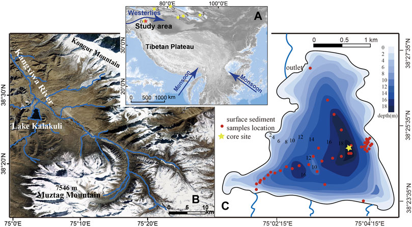
FIGURE 1. Maps of the study area. Map (A) shows the regional atmospheric circulation systems and the location of Lake Kalakuli (red star) in the Pamir Mountains. The yellow dots represent the main paleoclimatic records mentioned in the discussion (1. Bosten Lake; 2. Aibi Lake; 3. Issyk-Kul; 4. Barkol Lake; 5. Chaiwopu Lake; 6. Sate Baile Dikuli Lake). Map (B) shows Lake Kalakuli within its hydrological settings and the position of the Muztag Ata glacier. Map (C) shows the bathymetry of Lake Kalakuli with the locations of the sampling site for the master core (yellow star) and of the surface sediment samples (red dots) used to develop the diatom-based water depth transfer function.

Laboratory analyses

After transport to the laboratory, the core sections were split in two halves longitudinally. One half of the core was kept for XRF scanning while the other half was sectioned at 1 cm intervals. These samples were then vacuum freeze-dried prior to further laboratory analyses.

Dating

Radiocarbon dates were obtained on organic matter from 30 samples from different layers of the master core using accelerated mass spectroscopy (AMS). Eight measurements were carried out at the Xi’an Accelerator Mass Spectrometry Center, China, 5 at the Earth System Science Department, University of California, Irvine, USA and 17 at the Beta Analytic Inc., United States. The chronology of the uppermost 85 cm of the core was determined using the ²¹⁰Pb distribution calculated using the CRS (Constant Rate of Supply) model, together with the location of peaks in the distribution of ¹³⁷Cs (Appleby and Oldfield 1978).

Grain size and geochemical analyses

Grain size were measured with a Mastersizer 2000 laser particle size analyzer (Malvern Company, UK). The measurement range was 0.01–2000 μm, and the average particle size repeated measurement error was less than 3%. The grain size composition the Kalakuli sediments was divided into clay (<2 µm), silt (2–64 µm) and sand (>64 µm). Grain size data are missing for eight out of 45 surface sediment samples, while all samples collected from the master core (n = 1,533) were analyzed.

XRF scanning was carried out with an Itrax Core Scanner (Sweden) to determine the elemental content of the sediment core. The scanning was performed with a voltage of 30 kV, a current of 55 mA, and a scanning interval and time of 0.2 mm and 8 s, respectively. The element content is expressed as KCPS (Kilo-counter per second), which can only be used for a semi-quantitative analysis of the depth variation of each element, and cannot be used for quantitative description and comparison of the actual content of each element. XRF analysis was carried out at the Key Laboratory of the Tibetan Plateau Environmental Change and Land Surface Processes, CAS, in Beijing.

Diatom analysis

Diatom slides were prepared from about 0.05 g of freeze-dried sediment from all 45 surface sediment samples and from 159 of the core subsamples (i.e., about one every 10 cm along the core length). No less than 300 diatom valves were counted per sample under an Olympus BX53 light microscope with a ×1,000 magnification. For samples of the mastercore, due to the mass occurrence of Pantocsekiella comensis (syn. = Cyclotella comensis, = Lindavia comensis), fluctuations of the other species were obscured in some of the samples. In those cases, 200 more valves excluding P. comensis were counted with the final relative abundances calculated in proportion. This ensured higher confidence in the relative abundances of the secondary species while keeping a feasible workload. Diatoms were identified to the lowest taxonomic level possible using standard floras such as Krammer and Lange-Bertalot (1986), Krammer and Lange-Bertalot (1988), Krammer and Lange-Bertalot (1991a), Krammer and Lange-Bertalot (1991b) as well as articles dealing specifically with the flora from Lake Kalakuli (You et al., 2013; You et al., 2015; Peng et al., 2017; Zhang et al., 2017; Rioual et al., 2020). The nomenclature was updated following to the online database Algaebase (Guiry and Guiry, 2022). Diatom concentration in sediment core samples (i.e., the number of diatom valves per gram of dry sediment) was estimated by adding known quantities of divinyl benzene microspheres to the cleaned suspension (Battarbee and Kneen, 1982). To evaluate the preservation (and dissolution) of the diatom assemblages in core samples the F-index was calculated following Ryves et al. (2006). The F-index consists in the ratio between the well-preserved valves (i.e. unbroken valves showing no obvious signs of dissolution under the light microscope) and the total number of diatom valves counted. The F-index ranges between 0 (i.e. all the valves show signs of dissolution) and 1 (i.e. all valves are considered as pristine).

Statistical analyses

Surface sediment dataset

All diatom data are expressed as relative abundances. Cluster analysis using two-way indicator species analysis (TWINSPAN; Hill 1979) was used to determine the main diatoms assemblages composed by groups of surface sediment samples with homogeneous taxonomic composition. TWINSPAN is a top-down, divisive clustering method that is frequently used to classify biological community datasets, including diatom assemblages (Flower and Nicholson, 1987; Gesierich and Kofler, 2010; Mackay et al., 2012; Beauger et al., 2015; Feret et al., 2017). Species with number of occurrences <2 were excluded from the analysis. Due to the dominance of P. comensis in some samples, relative abundances of 0, 3, 4, 20 and 80% were used to define five pseudo-species cut levels instead of the default values of 0, 2, 5, 10 and 20%. Then, the clusters derived from TWINSPAN on the basis of the diatom communities were characterized further by drawing box-plots of their ranges of environmental variables (i.e. water depth and grain size), as done by Feret et al. (2017). Following this, the influences of these environmental variables on the diatom composition of the samples were assessed using redundancy analysis (RDA) with the eight samples missing grain-size data excluded from the analysis. In the RDA, redundant variables were removed by forward selection combined with Monte Carlo permutation tests and Bonferroni correction (p < 0.010; n = 999). The explanatory power and significance of each environmental variable in isolation (i.e. the marginal effect) were determined with a series of RDAs constrained with a single variable and with permutation test, while the unique (or partial) contribution of each variable was assessed using partial RDAs with covariables. Finally, a principal components analysis (PCA) was used to display in the same ordination space all the samples (n = 45), classified according TWINSPAN and contour plots of the important environmental gradients based on generalized additive models (GAM).

The relationship between the composition of the diatom assemblages and the water depth gradient was modelised using several methods including, simple weighted-averaging (WA), Modern Analogue (MAT), weighted-averaging partial-least-squares (WA-PLS) model and a Maximum Likelihood (ML) model. For all models (i.e. transfer functions) only diatom taxa that achieved >1% relative abundance in at least one surface sample were selected.

TWINSPAN was carried out using the free software WinTWINS v2.3 (Hill & Šmilauer 2005), the box-plots were drawn using R (R Core Team, 2019), the PCA and RDA were done in Canoco 5 (ter Braak and Šmilauer, 2012), and the transfer function models were developed using C2 version 1.7 (Juggins, 2014). In both PCA and RDA, diatom data were square root transformed to prevent species with extreme variance to have unduly large influence (ter Braak and Šmilauer 2012).

Sediment core dataset

Principal components analysis (PCA) was used to summarize the main directions of variation in the diatom assemblage data in the core. PCA was performed on square-root transformed diatom data using Canoco 5 (ter Braak and Šmilauer, 2012) and species abundance were graphed using C2 version 1.7 (Juggins, 2014). Stratigraphical zones were defined using CONISS, available in TILIA (https://www.tiliait.com/). Hill’s N2, commonly referred to as “effective” diversity (Hill, 1973), were calculated in C2 for the core assemblages and used as an indication of species evenness. Also using C2, the water transfer function derived from the surface sediment dataset was applied to the down-core diatom data to reconstruct past variations in water depth.

Results

Surface sediment dataset

In the 45 surface sediment samples retrieved from different water depth, 148 diatom species belonging to 56 genera were identified. The most frequent taxa are listed in Table 1 and plotted in Figure 2. Values of the Hill’s N2 vary from 6 to 27, with the less diverse samples and low eveness (N2<10) in the deepest samples, below 14.5 m.

TABLE 1

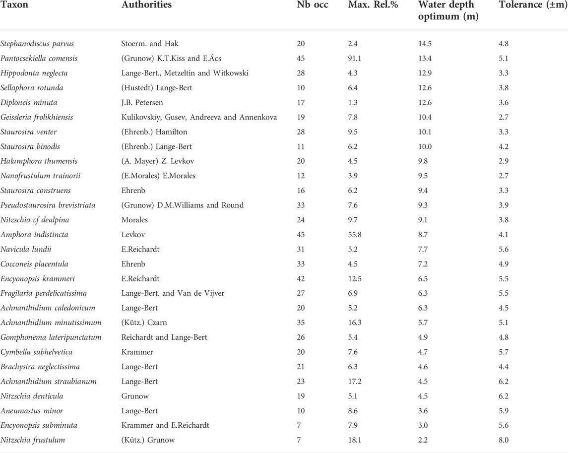
TABLE 1. Water depth optima and tolerance obtained from the WA-PLS model for the main species found in the surface sediment samples of Lake Kalakuli. Taxa are listed according to their water depth optima, in decreasing order.

FIGURE 2

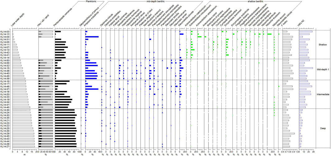
FIGURE 2. Relative percentages of the most abundant diatom taxa, F-index and Hill’s N2 index recorded in the surface sediment samples along the water depth gradient and the grain size data (i.e., percentages of clay, silt and sand). The dotted lines represent the diatom communities identified using cluster analysis (TWINSPAN). The intermediate zone includes samples belonging to the mid-depth and deep communities. Diatom taxa are ordered according to their observed distribution across the water depth gradient: on the left hand-side, in black, are planktonic taxa, in blue are benthic taxa occurring mostly in the mid-depth zone and in green are benthic taxa that mostly occur in the shallow, littoral zone.

The TWINSPAN classification dendrogram of the surface sediment diatom assemblages is shown in Figure 3 along with the box-plots of environmental variables for the groups defined by TWINSPAN. The first division splits the 45 samples into two communities distinguished by the water depth of the samples, with the 11 shallowest samples (with Achnanthidium minutissimum, Encyonopsis krammeri and Brachysira neglectissima as indicator species) on the positive side and the 34 deepest samples on the negative side (with Hippodonta neglecta as indicator species). The second division splits the group of 34 samples into two communities, with on the positive side 23 samples (group 3 on Figure 3) with Pantocsekiella comensis (abundance >20%) as indicator species and Stephanodiscus cf parvus as preferential, and on the negative side 11 samples (group 2 on Figure 3) with Amphora indistincta (>20%), Geissleria frolikhiensis (>4%), Staurosirella pinnata (>4%), Nitzschia cf dealpina (>3%) and Platessa ziegleri as indicator species. The box plots indicate that group 3 consists of samples taken generally at deeper water depth and with higher percentages of clay and silt and lower percentages of sand than the samples included in group 2. The third and last meaningful TWINSPAN division, distinguishes one sample (KL14-12) characterized by Staurosirella minuta as indicator species and Nitzschia frustulum (>4%) and Encyonopsis subminuta (>4%) as preferential from the other shallow samples that are included in group 1. Preferential species for group 1 include Pantocsekiella comensis (>4%), Encyonopsis krammeri (>3%), Cymbella subhelvetica, Fragilaria perdelicatissima, Cocconeis placentula and Nitzschia lacuum. The box-plots indicate that besides being associated with the shallowest water depth, samples in group 1 are characterized by low percentages of clay and silt and high percentages of sand.

FIGURE 3

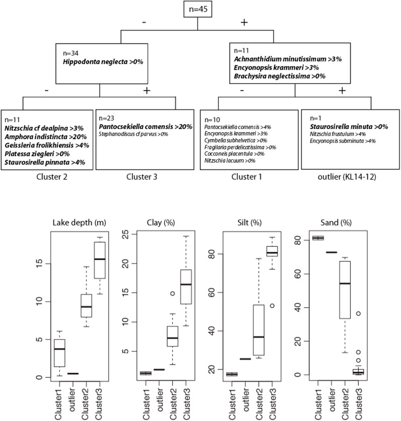
FIGURE 3. TWINSPAN classification dendrogram of the surface sediment diatom assemblages from Lake Kalakuli. Indicator species and their cut level are written in bold, while preferential species are written with normal font. Below the dendrogram are shown the box plots for water depth and grain size components for each diatom clusters defined by TWINSPAN. The 25th and 75th percent quartiles (excluding outliers) are drawn using a box, the median is shown with a horizontal line inside the box. The whiskers represent the upper and lower ‘inner fences’ that are drawn from the edge of the box up to the largest/lowest data point less than 1.5 times the box height. Outliers, i.e., values outside the inner fences, are shown as circles if they lie further from the edge of the box than three times the box height.

The RDA with forward selection determined that water depth and sand% significantly account for almost 40% of the variation in the diatom data (Figures 4A,B), while the other variables are redundant. RDA axis one is controlled by both the water depth and sand% with samples of group 1 on the right (shallow depth and high sand%), samples of group 3 on the left (high depth and low sand%) and samples of group 2 in a intermediate position (Figure 4A). The partial RDAs also show that both depth and sand% have significant unique contribution to the explained variation in the diatom data (p < 0.01, n = 999; Table 2) of 12.1 and 11.4%, respectively. In the PCA unconstrained ordination, for which all 45 samples could be displayed, the first two axes account for 41.3 and 14.3% of the variation in the species data, respectively (Table 2). Compared to the RDA, the positions of the groups in the PCA plots differ as axis one is now mainly associated with sand% while axis two is mainly associated with the depth gradient as shown by the contour plots (Figure 5).

FIGURE 4

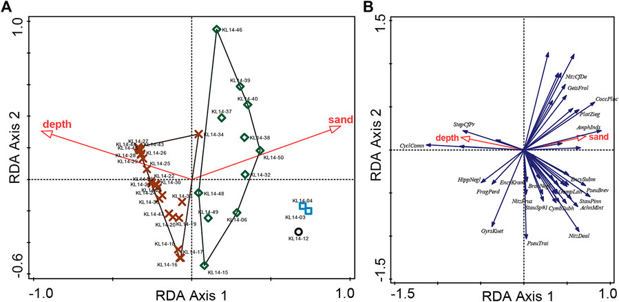
FIGURE 4. Redundancy analysis (RDA) of the surface sediment diatom dataset from Lake Kalakuli with (A) samples coded according to their TWINSPAN groupings and forward selection of the environmental variables (on the left) and (B) the most abundant species on the right (arrows). Only 37 samples, with a complete set of associated environmental variables were included in the analysis.

TABLE 2

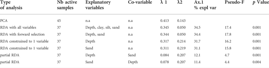
TABLE 2. Summary statistics for the multivariate analyses (PCA, RDAs, partial RDAs) performed on the Kalakuli surface sediment diatom dataset. Significance tests were performed with 999 Monte Carlo permutations.

FIGURE 5

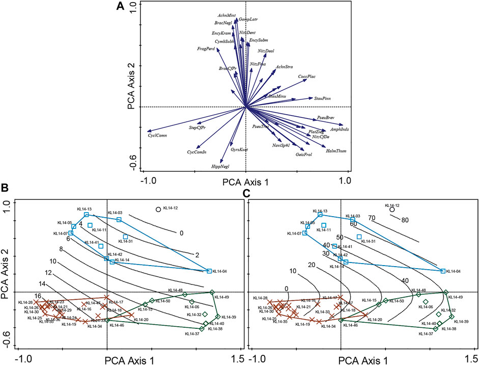
FIGURE 5. Principal components analysis (PCA) of the surface sediment diatom data. (A), shows the 45 most abundant species in the dataset (arrows). (B, C) show the samples coded according to their TWINSPAN groupings as well as the contour plots based on generalized additive models (GAM) for water depth and the percentage of sand in the samples, respectively. In this analysis all 45 surface sediment samples are included.

The three groups of surface sediment samples can be interpreted as depth communities as the box-plots, RDA and PCA show that water depth is the main environmental gradient driving the distribution of these diatom assemblages. These three communities distribute along the water depth gradient with an overlap between the mid-depth and deep water communities and can be described as follows:

(1) Deep water community (11–19 m): This community is found in the part of the basin that is the deepest and further away from the shore. The assemblages are almost exclusively composed of planktonic diatoms with P. comensis representing 80–90% of the assemblages. Stephanodiscus cf parvus, another planktonic species, is common. Hill’s N2 is very low (<10).

(2) Mid-depth community (6.5–14.5 m): This community is found in a depth zone that partly overlaps with that of the deep community. It is characterized by low light conditions and the absence of aquatic plants. The planktonic species P. comensis dominates in the deeper part and the benthic epipsammic species Amphora indistincta in the shallower part, respectively. The most abundant benthic species include several small Fragilariaceae such as Pseudostaurosira brevistriata, Staurosirella pinnata, Nanofrustulum trainorii, Staurosira construens, epipsammic diatoms such as Halamphora thumensis, Planothidium sp cf daui, Platessa ziegleri and epipelic diatoms such as Nitzschia cf dealpina, Geissleria frolikhiensis and Hippodonta neglecta. In addition, numerous benthic diatoms, predominantly nitzschoid and naviculoid taxa occur in low abundance in this zone and contribute to the high Hill’s N2 values of these assemblages.

(3) Shallow water community (below 6.5 m): This is the littoral zone of the lake characterized by the presence of aquatic plants and high light conditions. A large turnover among the benthic species distinguishes this community from the mid-depth community, with the disappearance of several of the species common in the previous community. Pantocsekiella comensis maintains the highest relative abundances (up to 50%). The most abundant benthic species include attached epiphytic taxa such as Achnanthidium minutissimum, Achnanthidium straubianum, Cocconeis placentula, Cymbella subhelvetica, Encyonopsis krammeri, Encyonopsis subminuta, Gomphonema lateripunctatum, the loosely attached colonial species Distrionella incognita, the epipsammic species Amphora indistincta, and numerous motile epipelic species including Aneumastus minor, Brachysira neglectissima, Nitzschia denticula, Nitzschia frustulum (Figure 2).

Diatom-water depth transfer function

The WAPLS component 2 model has a higher correlation coefficient (R² = 0.89) and a smaller error of prediction (RMSEP = 1.85 m) by comparison with the other models (Table 3), and was therefore selected for the transfer function. The residual errors however are quite high, ranging between +4.5 m for a sample taken in the shallow zone to -4.0 m for a sample taken at about 11 m water depth. There is also a bias toward an underestimation of the water depth at the end of the gradient (all samples with a water depth greater than 17 m) (Figure 6). Similar bias has been reported in previous studies on diatom-inferred water depth (Laird et al., 2011).

TABLE 3

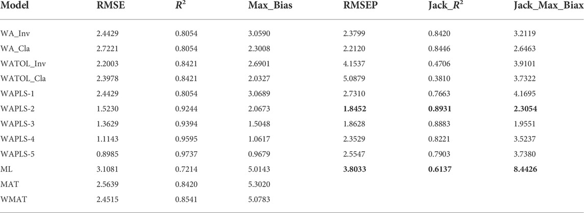
TABLE 3. Statistical performance of the weighted averaging partial least squares (WAPLS) model compared with other models for diatom-water depth transfer function from Lake Kalakuli.

FIGURE 6

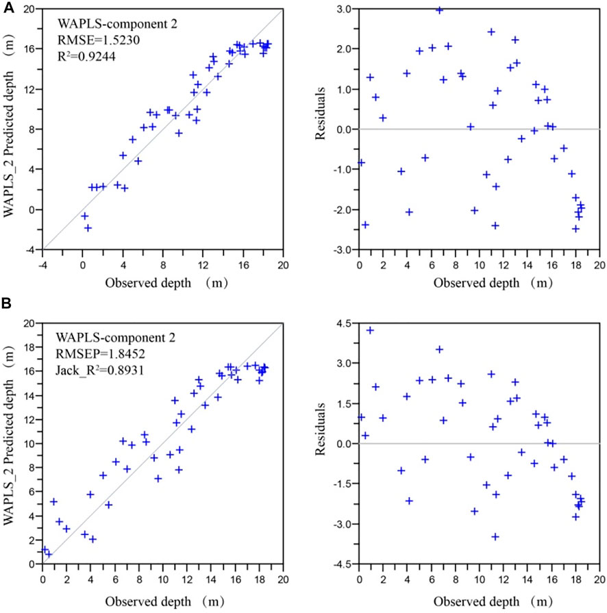
FIGURE 6. Lake Kalakuli diatom-based water depth model. Observed and predicted values of water depth and their residual errors for model WAPLS component 2 (A): apparent error, (B) Leave-one-out cross validation.

Chronology of the long core KL13-4

The development of the chronological model follows the guidelines proposed by Zhang et al. (2016) for radiocarbon-based age model of Holocene lake sediments in arid NW China. The 30 radiocarbon ages plot linearly against core depth suggesting a continuous sedimentary record (Table 4; Figure 7). A polynomial regression closely fits the depth-age relationship of core KL13-4 (R² = 0.9948) with the following equation:

$y=0.00000504x^3-0.00791433x^2+6.42070977x+1833.4$

TABLE 4

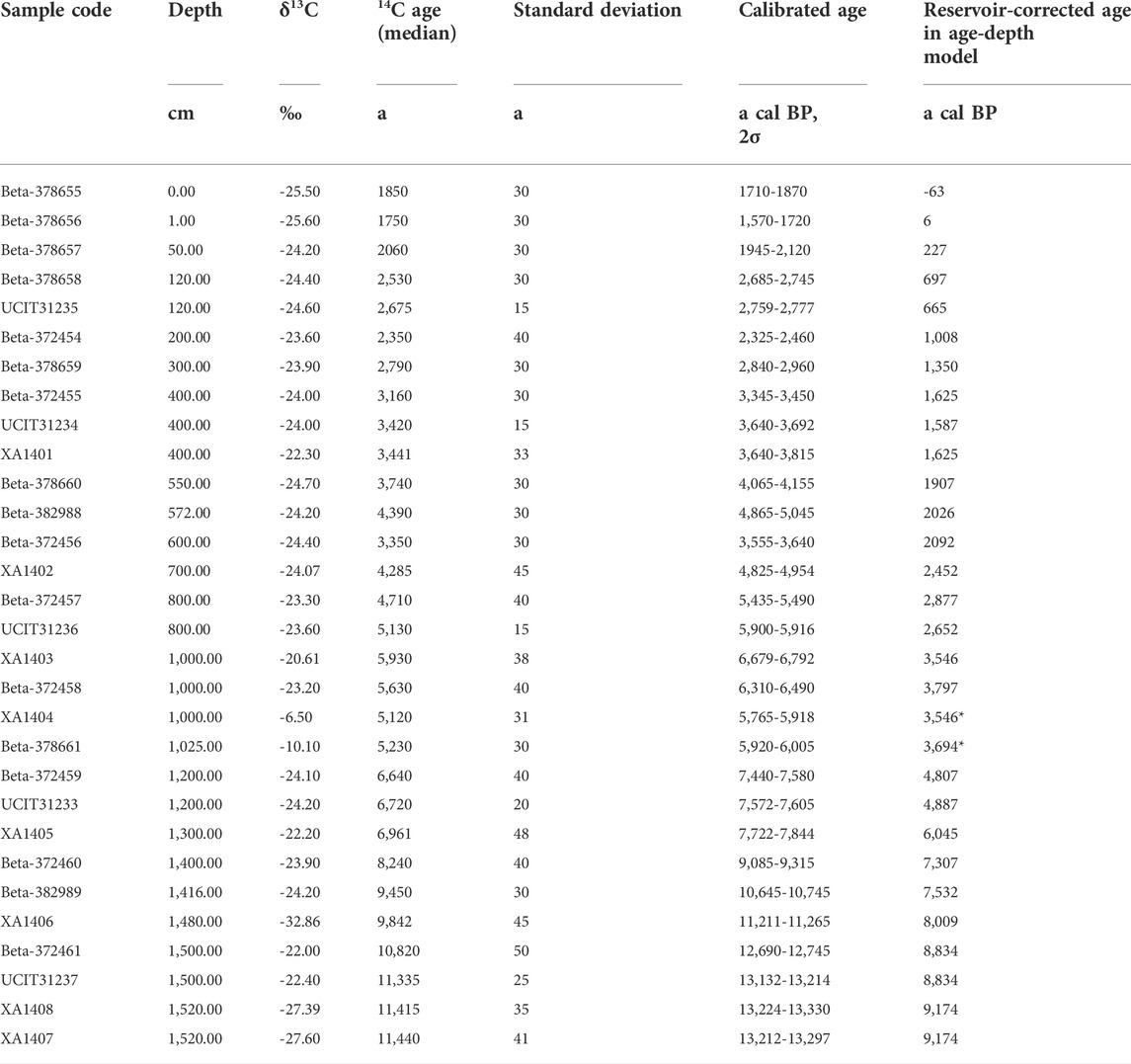
TABLE 4. Measured AMS¹⁴C ages and reservoir-corrected¹⁴C ages of dated samples from core KL13-4. *Dates excluded from the model.

FIGURE 7

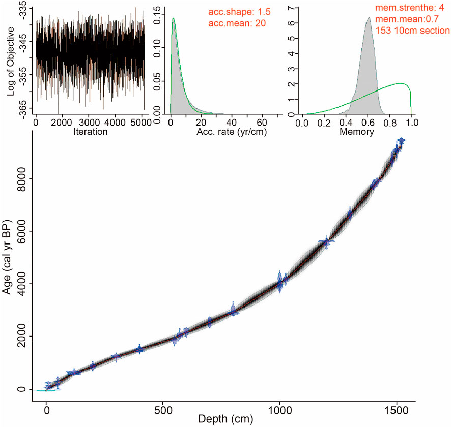
FIGURE 7. Age-depth model for the Lake Kalakuli sediment sequence KL13-4 produced by Bacon 2.2 (light blue symbols are ¹⁴C dates, the red dashed line shows the weighted mean ages and grey dashed lines show 95% confidence intervals).

The reservoir effect calculated based on the average deposition rate of ²¹⁰Pb_ex is 1983 years, and the old carbon age in Lake Kalakuli measured by Liu et al. (2014) is 1880 years. These two ages are very close to the solution of the polynomial equation for the top of the core, i.e. 1833 years. Therefore, this age can be regarded as the reservoir effect for the core KL13-4, while the curve derived from the regression represents changes in deposition rate (Zhang et al., 2016).

After correcting the carbon reservoir effect for the AMS ¹⁴C ages of all samples, ages were calibrated. The model resolution was 10 cm and calibrated using IntCal 13 data set (Reimer et al., 2013). The age-depth model was built in R with Bacon 2.2, using the Bayesian method (Blaauw and Christen, 2011). The ages are therefore reported as calibrated years (and/or thousand years) before present, set by convention at 1950 CE, using the following notation: a (ka) cal BP.

The age of 15.28 m at the bottom of the sequence is 9,831 a cal. BP, and the age of 15.33 m at the bottom of the drill hole is 9,880 a cal. BP by extrapolation of the deposition rate over the interval 15.20–15.28 m (Table 4; Figure 7).

Diatom assemblages of core KL 13-4

A total of 205 diatom taxa belonging to 58 genera were identified from the sediment core from the central basin of Lake Kalakuli. Amphora indistincta, Pantocsekiella comensis, Staurosira construens, Staurosirella pinnata and Staurosirella minuta are the only 5 species with abundance greater than 20% in at least one sample. The number of species per sample varies between 18 and 48, while the Hill’s N2 varies between 1.3 and 10.9. The samples showing the highest evenness (high N2) are in the bottom of the sequence, while the rest of the samples have low N2 (i.e. with low evenness and the dominance of a single species). The F-index ranges between 0.5 and 0.85 and is ∼0.7 on average (Figure 8). This indicates that although a large proportion of the diatoms contained in the sediment sequence show signs of dissolution, it can be assumed that the diatom record has no gap during which diatoms would have been completely dissolved. Dissolution is not a critical factor for this sequence.

FIGURE 8

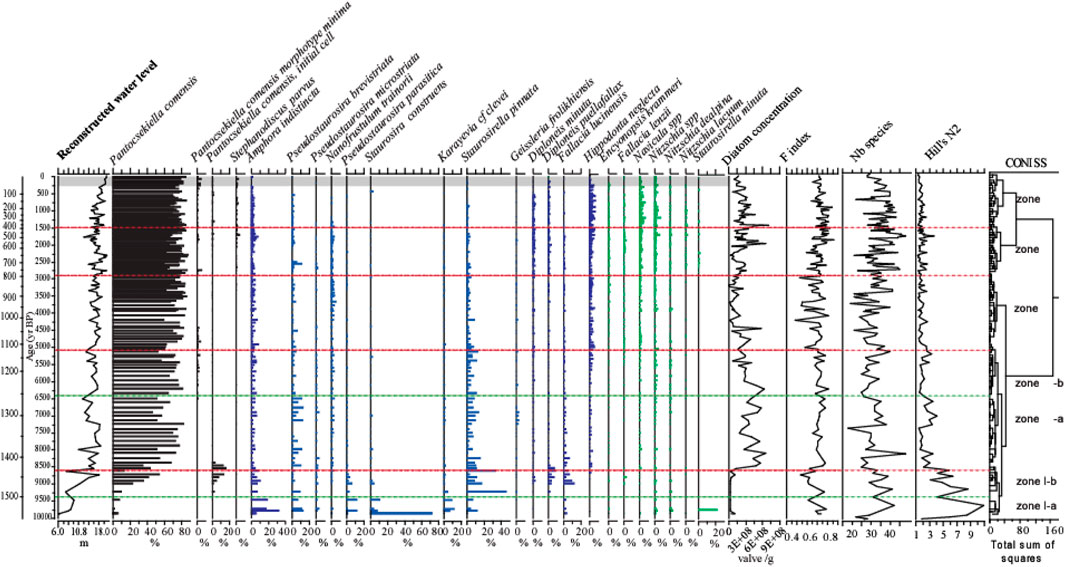
FIGURE 8. Summary diatom diagram for core KL 13-4. The curve on the left hand-side shows the reconstructed water level fluctuations derived from the diatom-water level transfer function developed for Lake Kalakuli. Diatom zones are based on a stratigraphically constrained cluster analysis (CONISS), main zones marked by red dashed lines, sub-zones marked by green dashed lines. The grey band at the top of the sequence symbolizes the modern conditions with a lake level highstand. Planktonic taxa are on the left of the diagram, from P. comensis to S. cf parvus, all other taxa are benthic and split according to their apparent preference for the mid-depth (in blue) and shallow zones (in green). On the right hand-side are plotted the diatom concentration in the sediment (as an indicator of diatom productivity), the F-index that estimates the preservation of the assemblages, the number of species found in each sample and the Hill’s N2 diversity index.

The first two axes of the PCA explain respectively 26.1% and 9.5% of the variance in the down-core diatom assemblages. On the ordination biplot for the first two PCA axes (Figure 9) the planktonic taxon P. comensis plots at the negative end of the first axis, while the benthic taxa A. indistincta, S. construens and S. pinnata plot at the positive end. This opposition between planktonic/benthic diatoms indicates that water level is the main environmental gradient influencing the assemblage composition of the sedimentary sequence. This is confirmed by the strong correlation (r² = 0.74) observed between the PCA scores on axis one and the water depth reconstruction derived from the WA-PLS model.

FIGURE 9

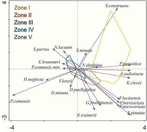
FIGURE 9. PCA ordination biplots showing the main diatom species (arrows) and samples from the sediment core KL 13–4 grouped into enveloped corresponding to the stratigraphical zones defined by CONISS cluster analysis.

The sequence could be divided into five zones using CONISS (Figure 8).

Zone I (1,533–1,441 cm, 9.9–8.5 cal ka BP):

Low diatom concentration (5.12×10⁷ valves/g) characterizes this zone, compared to the rest of the core. The zone can be divided into two sub zones: I-a (1,533–1,500 cm, 9.9–9.2 cal ka BP) and I-b (1,500–1,441 cm, 9.2–8.5 cal ka BP). Between 9.9 and 9.2 cal ka BP (Zone I-a), Fragilariaceae, small-sized benthic taxa with a preference for cold water, are dominant in the assemblages. The relative abundance of Staurosira construens at the bottom of the core is as high as 73%, with Amphora indistincta, Pseudostaurosira brevistriata, Pseudostaurosira parasitica, Staurosirella pinnata and Karayevia clevei also common. Pantocsekiella comensis is the only planktonic species and has a relative abundance below 10%. In Zone I-b, the abundances of Amphora indistincta, Pseudostaurosira brevistriata, Pseudostaurosira parasitica, Staurosira construens and Karayevia clevei declined while those of Diploneis puellafallax, Diploneis minuta and Fallacia lucinensis increase. At the same time, the planktonic species P. comensis becomes dominant. Initial valves of P. comensis are common.

Zone II (1,441–1,140 cm, 8.5–5.1 cal ka B.P.):

Total diatom concentration increased 4 times during the mid-Holocene, with an average of 2.16×10⁸ valves/g. Two subzones can be distinguished; II-a (1,441–1,260 cm, 8.5–6.4 cal ka BP) and II-b (1,260–1,030 cm, 6.4–5.1 cal ka BP). In Zone II-a, P. comensis has completely replaced benthic species as the dominant species, with an average relative abundance of 77% at 7.8–7.2 cal ka BP. There were decreases in small size benthic diatoms including Amphora indistincta, Staurosirella pinnata, Pseudostaurosira parasitica, Staurosira construens and Karayevia clevei, while a few benthic species with larger size, such as Geissleria frolikhiensis, Hippodonta neglecta and Navicula spp, began to appear in the core. In Zone II-b, P. comensis morphotype minima appeared. Pseudostaurosira brevistriata decreased significantly while Hippodonta neglecta and Nitzschia spp slightly increased.

Zone III (1,140–790 cm, 5.1–2.8 cal ka B.P.):

Diatom concentration fluctuated and generally decreased. P. comensis became even more dominant. Among benthic species the abundances of Amphora indistincta and small Fragilariaceae remain low while that of Hippodonta neglecta and Navicula spp increased.

Zone IV (790–400 cm, 2.8–1.5 cal ka B.P.):

Diatom concentration increased slightly, with an average of 2.16×10⁸ valves/g. P. comensis remains the dominant species with an average relative abundance of 75%. Stephanodiscus parvus began to appear. Among benthic species, small Fragilariaceae decreased further, while the genera Diploneis, Navicula and Nitzschia all showed small increases in diversity and abundance.

Zone V (400–0 cm, 1.5 cal ka B.P.):

Diatom concentration continues to increase with an average of 2.83×10⁸ valves/g. The dominant taxon for the most recent sediments of the core remains the planktonic P. comensis, maintaining abundances of up to 70% during the last 1,500 years. The relative abundance of benthic species Amphora indistincta and the small Fragilariaceae decline further during the last ∼500 years. Hippodonta neglecta, Navicula spp and Nitzschia spp dominate the benthic component of the assemblages.

Discussion

Modern diatom distribution and diversity across the water depth gradient in Lake Kalakuli

The diatom analysis of the surface sediment samples revealed three communities that distribute along the water depth gradient in Lake Kalakuli: 1) a deep water community (11–19 m), 2) a mid-depth community (6.5–14.5 m) and 3) a shallow water community (below 6.5 m). Similar distributions have been reported from various lakes across the world. For example in Lake Tovel, an oligotrophic mountain lake in Italy, Angeli and Cantonati (2005) also found maximum percentages of Staurosirella pinnata, Pseudostaurosira brevistriata and small Amphora in the mid-depth zone of this lake, while the deepest part was dominated by planktonic taxa (Cyclotella and Fragilaria spp in their case) and the shallow zone was dominated by a diverse assemblage of benthic species including Achnanthidium minutissimum, Brachysira, Encyonopsis and various motile Navicula. Also in Europe, Hofmann et al. (2020) observed in the subalpine Lake Oberer Soiernsee (Southern Germany), a shallow zone dominated by species of Achnanthidium, Encyonopsis, Brachysira with motile species of Navicula and Nitzschia and a deeper zone dominated by small Fragilariaceae and small Amphora. In North America, Laird et al. (2011), Kingsbury et al. (2012) and Gushulak and Cumming (2020) found consistently the same pattern in several lakes of northern Ontario (Canada), with Achnanthidium minutissimum being dominant in the shallow zone (<5 m depth) while Staurosirella pinnata and other small Fragilariaceae dominate the mid-depth zone. In China, the few studies that reported on the depth distribution of diatoms gave contrasting results. In Yulong Lake, an alpine lake in Yunnan (southern China), small Fragilariaceae are dominant throughout the shallow zone from 0 to 5.5 m, and remain abundant in the profundal zone (Zou et al., 2020). In Huguang Maar Lake, a volcanic lake in Guangzhou Province (S. China), Achnanthidium minutissimum and Encyonopsis spp dominate the shallow zone but only few Fragilariaceae are present and no clear mid-depth assemblage can be distinguished (Li et al., 2021). Finally, in Lugu Lake, a deep lake on the Yunnan Plateau, a mid-depth assemblage was observed but it was mainly composed of Diploneis species while the shallow zone (below 10 m depth) was dominated by small Fragilariaceae, with significant contribution of Achnanthidium minutissum, small Amphora and diverse motile species of Navicula and Nitzschia (Wang et al., 2012). These results suggest that some taxa have a rather specific distribution most likely driven by their tolerance to low light conditions, more than the actual depth of the water. However, the morphological profile of the depth-transects (e.g. steepness of the basin slope) and physicochemical characteristics of the lakes that are sampled greatly influence the depth distribution pattern of species from lake to lake (and even from transect to transect in some large, complex lakes) as already observed by Angeli and Cantonati (2005).

In Lake Kalakuli the bimodal distribution of P. comensis, which is completely dominant in the deep zone, very abundant in the shallow zone with a marked decrease in the mid-depth zone, suggests that this planktonic diatom habits in the shallow zone for a part of its life-cycle. The settling of live cells on the shallow sediment permits to the population of this species to survive summer periods of strong thermal stratification. Indeed, while cells in the deep zone will die if they settle in dark, deep waters below the photic zone, those deposited at shallow depth can remain alive and be quickly resuspended in the water column during periods of mixing. This allows this species to re-colonize the pelagic zone.

Generally, the littoral zone of a lake includes a variety of habitats such as rocks, sand, mud, and aquatic plants, which can provide a variety of substrates for diverse benthic diatoms to grow upon. By contrast, in deep water areas benthic diatoms cannot grow because not enough light reaches the bottom of the lake (Hayashi, 2011) and the assemblages that sediment below the water column are generally dominated by planktonic species that grow in the photic zone. As planktonic diatoms are generally much less diverse than benthic diatoms, such deep-water assemblages have low diversity. Therefore, over long time scales such as those recorded in the sedimentary record, a rise in lake water level may reduce the proportions of benthic species and thus the overall diatoms diversity found in the core assemblages.

Diatom-inferred water-level changes from Lake Kalakuli

The fossil diatom assemblage from the KL13-4 sediment core reveals several changes over the last ∼9.9 cal ka BP which, in combination with sediment–geochemical parameters, enables the reconstruction of major climate episodes and environmental conditions.

The diatom-based depth water reconstruction (Figure 8) shows that the lake depth varied between 6.1 and 17.5 m during the duration of the sequence. This reconstruction is an underestimation as we mentioned previously that the transfer function has a bias for the deep end of the depth gradient. However, as mentioned earlier the strength of the correlation between the PCA sample scores on axis-1 and the water depth reconstruction suggests that diatom-inferred depth is a good reflection of the assemblage changes. Thus, while the diatom-based water depth reconstruction should not be considered as an absolute record of lake level fluctuations, it is showing the general trends in lake level. The lake water level increased greatly from a low level in the Early Holocene. In the middle and late Holocene, water level fluctuated slightly with a slight upward trend while in the last few hundred years, it has increased significantly, and is now at its highest.

Fossil diatoms at the bottom of Lake Kalakuli sequence recorded a low lake water level, about 13 m below the current level. During the late Pleistocene (16-11 ka BP), glaciers including those from the Muztagh Ata and Kongur Shan, advanced in the alpine regions of Central Asia (Sevastyanov et al., 1990). The climate was cold and dry, causing a decrease input of glacier melt water, and a large number of lakes dried up or even disappeared. The total abundance of diatoms was very low, and the assemblages mainly consisted of small fragilarioid taxa, which are often reported to represent pioneer diatom communities (Väliranta et al., 2011) in early postglacial tundra environments. These species prefer poor light conditions (Anderson, 2000), oligotrophic and alkaline conditions with cold temperatures and short growing seasons (Laing et al., 1999; Biskaborn et al., 2012). Their highest abundances are reached at water temperatures below approximately 6 °C (Joynt and Wolfe, 2001). We could infer a cold lake environment with long seasonal ice cover.

In the early Holocene, as temperature rose, the glaciers receded and this resulted in large increase in the influx of glacial melt water and coarse mineral particles into the lake basin. As a result, the clay mineral content at the bottom of the core was low (Figure 10). As reported for other alpine lakes in the region (Chen et al., 2008), Lake Kalakuli started to refill during this period, and lake levels fluctuated before stabilizing. Two sudden drops in water level occurred at 8.7 and 8.2 cal ka BP, which may be related to the Muztag Ata glacier advance at around 8.4 ka (Seong et al., 2009). The diatom concentration and relative abundance of planktonic species were quite low during this period, most likely due to the low water level of the lake that limited the space available for planktonic diatoms to grow, as well as the low water temperature associated with large influx of glacial meltwater, which is not conducive to the massive growth of diatoms. Interestingly, the benthic species that dominate the bottom part of the sequence are part of the mid-depth community in the modern lake while few species forming the modern shallow zone community are present. This suggests that aquatic plants were absent and light conditions were low, in agreement with large supply of cold and turbid glacial meltwater.

FIGURE 10

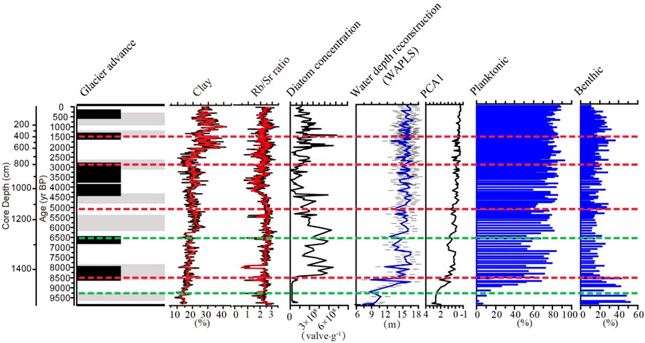
FIGURE 10. Record of glacier advance from Seong et al. (2009), on the left hand-side, compared with geochemical and diatom data derived from the Lake Kalakuli sequence. From left to right: percentage of clay, Rb/Sr ratio, diatom concentration, diatom sample scores on PCA axis-1 (x-axis is reversed), diatom-based water depth reconstruction (with error bars corresponding to the RMSEP as dashed lines, in grey) and relative abundances of planktonic and benthic diatoms plotted against core depth and chronology. The red and green dashed lines indicate the diatom assemblage zones and subzones, respectively (see caption of Figure 8 for details).

In the Mid-Holocene (∼8–4 cal ka BP), water level returned to high levels and the average abundance of diatoms at this stage is the highest of the Holocene, reflecting a more productive lake, associated with a warm and humid climate in the East Pamir during that period, corresponding to the Holocene warm period in China (Shi et al., 1992; An et al., 1993). Although the climatic conditions were relatively stable during this stage, there were fluctuations around 7.2–6.5 cal ka BP, 5.0 cal ka BP, and 4.2 cal ka BP, which were manifested in the decrease of lake water level and slight increase in the diversity index Hill’s N2 (Figure 8). The records of ¹⁰Be terrestrial cosmogenic nuclide surface exposure dating of moraines indicate that glacier advanced around 7.0–6.5 cal ka BP and 4.2 cal ka BP (Seong et al., 2009) (Figure 10). Thus, the lowering of the lake water level during this period was probably related to the advancement of glaciers that reduced the supply of melt water. From the perspective of diatom productivity, the diatom concentration during the periods of 7.2–6.5 cal ka BP and 5.0 ka BP was lower than the average value of the warm period, while the diversity increased during the same period.

In the late Holocene (∼4 cal ka BP to the present), the lake level fluctuates frequently but with low amplitude. During this period, three periods of glacier advance and two periods of retreat are recorded (Seong et al., 2009). During this period, there is a noticeable increase in the percentages of motile diatoms such as Hippodonta neglecta, Navicula spp and Nitzschia spp. that correspond with the large increase in clay content in the core (Figures 8, 10). With such influx of fine sediment, benthic diatoms that can move and avoid burial are favored over non-motile diatoms (Jones et al., 2014). The rise of the lake water level in modern times may be related to climate warming caused by human activities and increase in the supply of glacial melt water.

Regional comparison and climatic significance

According to the trends in water level in Lake Kalakuli, the evolution of the lake can be roughly divided into three stages: the rising period of the water level in the Early Holocene, the relatively stable period of the mid-late Holocene, and the modern rising period. This trend can be compared with the climate records of the westerlies-dominated region in Central Asia.

During the early Holocene period before 8.0 cal ka BP in the Kalakuli region, the climate was relatively arid but effective moisture was increasing. Studies on other lakes from the arid regions of Central Asia also reflect a cool and dry environment and low lake levels during the early Holocene, which are in good agreement with the climate characteristics revealed by the Kalakuli records. For example, Bosten Lake, once the largest freshwater lake in inland China, was still dry before 8.4 cal ka BP (Huang et al., 2009); Lake Aibi, situated in the western margin of Junggar Basin, was a marsh or wetland between 13.9-7.4 ka BP (Wang et al., 2013); Lake Issyk-Kul, located on the west side of the Tianshan Mountains, was also formed at around 8 cal ka BP (Ricketts et al., 2001). Analyses based on δ¹⁸O, δ¹³C and grain size from Barkol Lake also show relatively arid conditions in the early Holocene (9.4–7.4 ka BP) (Xue and Wei, 2011).

In the middle and late Holocene, the water level of the Lake Kalakuli was steady with a slight upward trend, reflecting the continuous increase of effective humidity in the area since the Holocene. Wang and Feng (2013) based on the integrated humidity curve of four lakes located in northern Xinjiang, also show that humidity increased from 8 cal ka BP. The records of Barkol Lake (An et al., 2012), the peat records of Chaiwopu in central Xinjiang (Hong et al., 2014), and the pollen records of the Caspian Sea (Leroy et al., 2014) all reflect the same climatic characteristics as in the Kalakuli region. In their review, Chen et al. (2008) and Mathis et al. (2014) summarized the trends observed for the lakes located in the westerlies region of Central Asia that the highest lake level occurred in the Mid-Holocene, corresponding to the humid environment, and the lake level decreased in the late Holocene as the climate gradually became dry. Pollen (Huang et al., 2009) and aeolian sedimentary records (Long et al., 2014) also show that the inland area of ​​Asia was very arid in the early Holocene, then reached the wettest state in the Middle Holocene after a rapid increase in moisture at about 8 ka BP, and gradually began to dry out in the late Holocene. The water level trend of Lake Kalakuli is therefore completely consistent with the climate evolution of the region as described in the literature.

Driving mechanisms of climate variation

This pattern of an early Holocene dry phase and a mid-late Holocene humid climate has universal significance in the inland westerlies region of Central Asia. The early Holocene drought in the inland westerlies region of Asia is considered to be related to the high solar radiation in the northern hemisphere in summer as radiation increases the temperature (Kutzbach and Guetter, 1986; Berger and Loutre, 1991), narrowing the difference between the high and low latitudes. The temperature difference between the latitudes and the subtropical high caused the subtropical high to move northward and strengthen, the westerlies belt moved northward and the intensity of the westerlies jet stream decreased, and the activity of mid-latitude cyclones also weakened. At the same time, the injection of a large amount of melt water from the Laurentide Ice Sheet into the North Atlantic made the sea surface water temperature (SST) lag behind. The lower water vapor evaporation in the North Atlantic then leads to a reduction in the amount of water vapor carried by the westerlies wind (Carlson et al., 2008). In addition, the strong radiation also caused an increase in the sinking airflow on the northern edge of the Qinghai-Tibet Plateau. Therefore, these changes of solar radiation in the northern hemisphere in summer led to less precipitation and more evaporation in the westerlies region of Central Asia in the Early Holocene. During the Lateglacial period and the Younger Dryas (YD) event, the Muztag Ata glacier advanced, and the glacier melt water was reduced dramatically or even dried up, which caused extremely low lake level in the early Holocene. After the YD event, rapid warming caused the melting of alpine glaciers, and the rapid rise of the Lake Kalakuli water level at ∼8.0 ka BP.

In the mid-late Holocene, solar radiation in the northern hemisphere decreased, which increased the temperature difference between high and low latitudes. The weakened subtropical high moved south, which led to the southward movement and increasing intensity of the westerlies jet, while the activity of mid-latitude cyclones also increased (Magny et al., 2007). At the same time, around 8.0 ka BP, the volume of the Laurentide ice sheet had shrunk to 10% of the peak area reached during the Last Glacial Maximum, and completely disappeared at 6.0 cal ka BP (Dyke et al., 2013). Then, the North Atlantic SST gradually increased to the highest value of the Holocene, and so the water vapor brought into Central Asia with the westerlies winds also gradually increased. During the mid-Holocene, water level fluctuations and the diatom productivity record reflect the “cold wet/warm dry” hydrothermal configuration pattern, which may be due to the northward movement of the westerlies belt in the warm period, the weakening of the strength of the westerlies jet, and the reduced activity of mid-latitude cyclones, as well as increased evaporation caused by temperature rise, and vice versa.

The temperature changes reflected by the organic carbon content of the sediments of Lake Sate Baile Dikuli, located next to Lake Kalakuli (Li et al., 2018) and the temperature record of the northeastern Qinghai-Tibet Plateau (Wang et al., 2015) both show that the rapid warming at the end of the 20th century was the highest in the past 200 years. Such rapid temperature increase has triggered a rapid response of mountain glaciers, especially in the Qinghai-Tibet Plateau glacial area (Duan et al., 2007). Therefore, the water level rise in Lake Kalakuli in recent years can be regarded as a direct manifestation of the large amount of meltwater caused by the loss of ice in the Muztag Ata glacier, where the magnitude of warming is extremely large, around 2.0–2.4°C per decade according to the δ¹⁸O record from the Muztag Ata ice core (Tian et al., 2006).

Conclusion

Diatom assemblage variations in Lake Kalakuli show that the trends in climate in this area are basically consistent with climate evolution in the westerlies region of Central Asia. In the early Holocene, the lake water level was the lowest for the entire Holocene and rose after 9 cal ka BP. In the middle and late Holocene, the lake level was relatively stable with only small fluctuations, and the overall trend was a slight increase. These results show that effective humidity in this area was low and increased rapidly in the early Holocene; the humidity was higher in the middle and late Holocene. In the last 200 years, the lake level increased significantly and reached the highest value for the whole sequence, which may be related to the increase supply of glacier melt water caused by global warming. The fundamental driving mechanism of the moisture and temperature changes of arid Asia during the Holocene is the change of westerlies circulation caused by changes in solar radiation, while the Muztag Ata glacier activity has a direct and key impact on the change of the lake water level.

Data availability statement

The original contributions presented in the study are included in the article/supplementary material, further inquiries can be directed to the corresponding authors.

Author contributions

YP: conceptualization, methodology, analysis, and writing–original manuscript. PR: statistical analysis, writing, reviewing and editing. ZJ: supervision, project administration and funding acquisition. All authors contributed to the article and approved the submitted version.

Funding

ZJ acknowledges his current support from the Research Center for Ecology and Environment of Central Asia, CAS and CAS Strategic Priority Research Program (XDA2007010202). PR acknowledges his current support from the Strategic Priority Research Program of the Chinese Academy of Sciences (grant No XDB 26000000). YP acknowledges her current support from the National Natural Science Foundation of China (grant No 42102233), the National Natural Science Foundation of Hunan Province, China (grant No 2020JJ5518), and the Research Foundation of Education Bureau of Hunan Province, China (grant No 19C1669).

Conflict of interest

The authors declare that the research was conducted in the absence of any commercial or financial relationships that could be construed as a potential conflict of interest.

Publisher’s note

All claims expressed in this article are solely those of the authors and do not necessarily represent those of their affiliated organizations, or those of the publisher, the editors and the reviewers. Any product that may be evaluated in this article, or claim that may be made by its manufacturer, is not guaranteed or endorsed by the publisher.

Acknowledgments

We are grateful to Zhang Fei from the Institute of Earth Environment, Chinese Academy of Sciences and Xie Ying from the Institute of Tibetan Plateau Research, Chinese Academy of Sciences for their help with field work. We also thank the reviewers and the editor for their constructive comments that helped us improve our manuscript.

References

Aichner, B., Feakins, S. J., Lee, J. E., Herzschuh, U., and Liu, X. Q. (2015). High-resolution leaf wax carbon and hydrogen isotopic record of the late Holocene paleoclimate in arid Central Asia. Clim. Past. 11, 619–633. doi:10.5194/cp-11-619-2015

CrossRef Full Text | Google Scholar

An, Z., Bott, S., Wu, X. H., Kutzbach, J., Wang, S. M., Liu, X. D., et al. (1993). Holocene optimum and east monsoon change in middle-east China. Chin. Sci. Bull. 38, 1302–1305.

Google Scholar

An, C. B., Lu, Y. B., Zhao, J. J., Tao, S. C., Dong, W. M., Li, H., et al. (2012). A high-resolution record of Holocene environmental and climatic changes from Lake Balikun (Xinjiang, China): Implications for central Asia. Holocene 22 (1), 43–52. doi:10.1177/0959683611405244

CrossRef Full Text | Google Scholar

Anderson, N. J. (2000). Miniview: Diatoms, temperature and climatic change. Eur. J. Phycol. 35, 307–314. doi:10.1080/09670260010001735911

CrossRef Full Text | Google Scholar

Angeli, M., and Cantonati, M. (2005). Depth-distribution of surface sediment diatoms in Lake Tovel, Italy. SIL Proc. 1922-2010 29 (1), 539–544. doi:10.1080/03680770.2005.11902072

CrossRef Full Text | Google Scholar

Appleby, P. G., and Oldfield, F. (1978). The calculation of lead-210 dates assuming a constant rate of supply of unsupported 210Pb to the sediment. Catena 5 (1), 1–8. doi:10.1016/s0341-8162(78)80002-2

CrossRef Full Text | Google Scholar

Battarbee, R. W., and Kneen, M. J. (1982). The use of electronically counted microspheres in absolute diatom analysis. Limnol. Oceanogr. 27 (1), 184–188. doi:10.4319/lo.1982.27.1.0184

CrossRef Full Text | Google Scholar

Beauger, A., Delcoigne, A., Voldoire, O., Serieyssol, K., and Peiry, J.-L. (2015). Distribution of diatom, macrophyte and benthic macroinvertebrate communities related to spatial and environmental characteristics: The example of a cut-off meander of the river allier (France). Cryptogam. Algol. 36 (3), 323–355. doi:10.7872/crya/v36.iss3.2015.323

CrossRef Full Text | Google Scholar

Berger, A., and Loutre, M. F. (1991). Insolation values for the climate of the last 10 million years. Quat. Sci. Rev. 10 (4), 297–317. doi:10.1016/0277-3791(91)90033-Q

CrossRef Full Text | Google Scholar

Biskaborn, B. K., Herzschuh, U., Bolshiyanov, D., Savelieva, L., and Diekmann, B. (2012). Environmental variability in northeastern Siberia during the last ∼ 13,300 yr inferred from lake diatoms and sediment-geochemical parameters. Palaeogeogr. Palaeoclimatol. Palaeoecol. 329-330, 22–36. doi:10.1016/j.palaeo.2012.02.003

CrossRef Full Text | Google Scholar

Blaauw, M., and Christen, J. A. (2011). Flexible paleoclimate age-depth models using an autoregressive gamma process. Bayesian Anal. 6 (6), 457–474. doi:10.1214/ba/1339616472

CrossRef Full Text | Google Scholar

Bond, G., Showers, W., Cheseby, M., Lotti, R., Almasi, P., deMenocal, P., et al. (1997). A pervasive millennial-scale cycle in North Atlantic Holocene and glacial climates. Science 278, 1257–1266. doi:10.1126/science.278.5341.1257

CrossRef Full Text | Google Scholar

Carlson, A. E., LeGrande, A., Oppo, D. W., Came, R. E., Schmidt, G. A., Anslow, F. S., et al. (2008). Rapid early Holocene deglaciation of the Laurentide ice sheet. Nat. Geosci. 1, 620–624. doi:10.1038/ngeo285

CrossRef Full Text | Google Scholar

Chen, F. H., Yu, Z. C., Yang, M. L., Ito, E., Wang, S. M., Madsen, D. B., et al. (2008). Holocene moisture evolution in arid central Asia and its out-of-phase relationship with Asian monsoon history. Quat. Sci. Rev. 27 (3-4), 351–364. doi:10.1016/j.quascirev.2007.10.017

CrossRef Full Text | Google Scholar

Chen, F. H., Chen, J. H., Huang, W., Chen, S. Q., Huang, X. Z., Jin, L. Y., et al. (2019). Westerlies Asia and monsoonal Asia: Spatiotemporal differences in climate change and possible mechanisms on decadal to sub-orbital timescales. Earth-Science Rev. 192, 337–354. doi:10.1016/j.earscirev.2019.03.005

CrossRef Full Text | Google Scholar

Cheng, H., Spötl, C., Breitenbach, S. F. M., Sinha, A., Wassenburg, J. A., Jochum, K. P., et al. (2016). Climate variations of Central Asia on orbital to millennial timescales. Sci. Rep. 6, 36975. doi:10.1038/srep36975

PubMed Abstract | CrossRef Full Text | Google Scholar

Chiba, T., Endo, K., Sugai, T., Haraguchi, T., Kondo, R., Kubota, J., et al. (2016). Reconstruction of Lake Balkhash levels and precipitation/evaporation changes during the last 2000 years from fossil diatom assemblages. Quat. Int. 397, 330–341. doi:10.1016/j.quaint.2015.08.009

CrossRef Full Text | Google Scholar

Duan, K. Q., Yao, T. D., Wang, N. L., Tian, L. D., Xu, B. Q., and Wu, G. J. (2007). Records of precipitation in the Muztag Ata ice core and its climate significance to glacier water resources. J. Glaciol. Geocryol. 29 (5), 680–684. doi:10.3969/j.issn.1000-0240.2007.05.002

CrossRef Full Text | Google Scholar

Dyke, A. S., Moore, A., and Robertson, L. (2003). “Deglaciation of north America,” in Geological survey of Canada open file, 1574. doi:10.4095/214399

CrossRef Full Text | Google Scholar

Feret, L., Bouchez, A., and Rimet, F. (2017). Benthic diatom communities in high altitude lakes: A large scale study in the French alps. Ann. Limnol. - Int. J. Lim. 53, 411–423. doi:10.1051/limn/2017025

CrossRef Full Text | Google Scholar

Flower, R. J., and Nicholson, A. J. (1987). Relationships between bathymetry, water quality and diatoms in some Hebridean lochs. Freshw. Biol. 18, 71–85. doi:10.1111/j.1365-2427.1987.tb01296.x

CrossRef Full Text | Google Scholar

Gesierich, D., and Kofler, W. (2010). Epilithic diatoms from rheocrene springs in the eastern alps (vorarlberg, Austria). Diatom Res. 25 (1), 43–66. doi:10.1080/0269249x.2010.9705828

CrossRef Full Text | Google Scholar

Guiry, M. D., and Guiry, G. M. (2022). AlgaeBase. World-wide electronic publication. Galway: National University of Ireland. Available at: https://www.algaebase.org.

Google Scholar

Gushulak, C. A. C., and Cumming, B. F. (2020). Diatom assemblages are controlled by light attenuation in oligotrophic and mesotrophic lakes in northern Ontario (Canada). J. Paleolimnol. 64, 419–433. doi:10.1007/s10933-020-00146-w

CrossRef Full Text | Google Scholar

Hayashi, T. (2011). Monospecific planktonic diatom assemblages in the Paleo-Kathmandu Lake during the middle Brunhes Chron: Implications for the paradox of the plankton. Palaeogeogr. Palaeoclimatol. Palaeoecol. 300 (1), 46–58. doi:10.1016/j.palaeo.2010.12.007

CrossRef Full Text | Google Scholar

Herzschuh, U., Cao, X., Laepple, T., Dallmeyer, A., Telford, R. J., Ni, J., et al. (2019). Position and orientation of the westerly jet determined Holocene rainfall patterns in China. Nat. Commun. 10, 2376. doi:10.1038/s41467-019-09866-8

PubMed Abstract | CrossRef Full Text | Google Scholar

Hill, M. O. (1973). Diversity and evenness: A unifying notation and its consequences. Ecology 54, 427–432. doi:10.2307/1934352

CrossRef Full Text | Google Scholar

Hill, M. O., and Šmilauer, P. (2005). TWINSPAN for Windows version 2.3. České Budějovice: Centre for Ecology & Hydrology and University of South Bohemia.

Google Scholar

Hill, M. O. (1979). “Twinspan: A fortran program for arranging multivariate data in an ordered two-way table by classification of the individuals and attributes,” in Section of Ecology and systematics (Ithaca, NY: Cornell University), 106.

Google Scholar

Hofmann, A. M., Geist, J., Nowotny, L., and Raeder, U. (2020). Depth-distribution of Lake benthic diatom assemblages in relation to light availability and substrate: Implications for paleolimnological studies. J. Paleolimnol. 64 (3), 315–334. doi:10.1007/s10933-020-00139-9

CrossRef Full Text | Google Scholar

Holzer, N., Vijay, S., Yao, T., Xu, B., Buchroithner, M., Bolch, T., et al. (2015). Four decades of glacier variations at Muztagh Ata (eastern Pamir): A multi-sensor study including hexagon KH-9 and pléiades data. Cryosphere 9 (2), 2071–2088. doi:10.5194/tc-9-2071-2015

CrossRef Full Text | Google Scholar

Hong, B., Gasse, F., Uchida, M., Hong, Y. T., Leng, X. T., Shibata, Y., et al. (2014). Increasing summer rainfall in arid eastern-Central Asia over the past 8500 years. Sci. Rep. 4, 5279. doi:10.1038/srep05279

PubMed Abstract | CrossRef Full Text | Google Scholar

Huang, X. Z., Chen, F. H., Fan, Y. X., and Yang, M. L. (2009). Dry late-glacial and early Holocene climate in arid central Asia indicated by lithological and palynological evidence from Bosten Lake, China. Quat. Int. 194, 19–27. doi:10.1016/j.quaint.2007.10.002

CrossRef Full Text | Google Scholar

Jones, J. I., Duerdoth, C. P., Collins, A. L., Naden, P. S., and Sear, D. A. (2014). Interactions between diatoms and fine sediment. Hydrol. Process. 28, 1226–1237. doi:10.1002/hyp.9671

CrossRef Full Text | Google Scholar

Joynt III, E. H., and Wolfe, A. P. (2001). Paleoenvironmental inference models from sediment diatom assemblages in Baffin Island lakes (Nunavut, Canada) and reconstruction of summer water temperature. Can. J. Fish. Aquat. Sci. 58 (6), 1222–1243. doi:10.1139/f01-071

CrossRef Full Text | Google Scholar

Juggins, S. (2014). C2 version 1.7. Available at: https://www.staff.ncl.ac.uk/stephen.juggins/software/C2Home.html.

Google Scholar

Kingsbury, M. V., Laird, K. R., and Cumming, B. F. (2012). Consistent patterns in diatom assemblages and diversity measures across water-depth gradients from eight Boreal lakes from north-Western Ontario (Canada). Freshw. Biol. 57 (6), 1151–1165. doi:10.1111/j.1365-2427.2012.02781.x

CrossRef Full Text | Google Scholar

Krammer, K., and Lange-Bertalot, H. (1986). “Bacillariophyceae: Naviculaceae,” in Süsswasserflora von Mitteleuropa. Bd. 2, teil 1. Editors H. Ettl, J. Gerloff, H. Heynig, and D. Mollenhauer (Stuttgart: Gustav Fischer).

Google Scholar

Krammer, K., and Lange-Bertalot, H. (1988). “Bacillariophyceae: Bacillariaceae, epithemiaceae, surirellaceae,” in Süsswasserflora von Mitteleuropa. Bd. 2, teil 2. Editors H. Ettl, J. Gerloff, H. Heynig, and D. Mollenhauer (Stuttgart: Gustav Fischer).

Google Scholar

Krammer, K., and Lange-Bertalot, H. (1991a). “Bacillariophyceae: Centrales, Fragilariaceae, eunotiaceae,” in Süsswasserflora von Mitteleuropa. Bd. 2, teil 3. Editors H. Ettl, J. Gerloff, H. Heynig, and D. Mollenhauer (Stuttgart: Gustav Fischer).

Google Scholar

Krammer, K., and Lange-Bertalot, H. (1991b). “Bacillariophyceae: Achnanthaceae, Kritische Ergänzungen zu Navicula (Lineolatae) und Gomphonema Gesamtliterarurverzeichnis,” in Süsswasserflora von Mitteleuropa. Bd. 2, teil 4. Editors H. Ettl, J. Gerloff, H. Heynig, and D. Mollenhauer (Stuttgart: Gustav Fischer).

Google Scholar

Kutzbach, J. E., and Guetter, P. J. (1986). The influence of changing orbital parameters and surface boundary conditions on climate simulations for the past 18 000 years. J. Atmos. Sci. 43 (16), 1726–1759. doi:10.1175/1520-0469(1986)043<1726:tiocop>2.0.co;2

CrossRef Full Text | Google Scholar

Laing, T. E., Rühland, K. M., and Smol, J. P. (1999). Past environmental and climatic changes related to tree-line shifts inferred from fossil diatoms from a lake near the Lena River Delta, Siberia. Holocene 9, 547–557. doi:10.1191/095968399675614733

CrossRef Full Text | Google Scholar

Laird, K. R., Kingsbury, M. V., Lewis, C. F. M., and Cumming, B. F. (2011). Diatom-inferred depth models in 8 Canadian boreal lakes: Inferred changes in the benthic:planktonic depth boundary and implications for assessment of past droughts. Quat. Sci. Rev. 30, 1201–1217. doi:10.1016/j.quascirev.2011.02.009

CrossRef Full Text | Google Scholar

Leroy, S. A. G., López-Merino, L., Tudryn, A., Chalié, F., and Gasse, F. (2014). Late Pleistocene and Holocene palaeoenvironments in and around the middle Caspian basin as reconstructed from a deep-sea core. Quat. Sci. Rev. 101 (5), 91–110. doi:10.1016/j.quascirev.2014.07.011

CrossRef Full Text | Google Scholar

Li, Y., Rioual, P., Shen, S., and Xiao, X. Y. (2015). Diatom response to climatic and tectonic forcing of a palaeolake at the southeastern margin of the Tibetan Plateau during the late Pleistocene, between 140 and 35ka BP. Palaeogeogr. Palaeoclimatol. Palaeoecol. 436 (3), 123–134. doi:10.1016/j.palaeo.2015.06.039

CrossRef Full Text | Google Scholar

Li, S. H., Jin, Z. D., Zhang, F., Zhang, X. L., Xie, Y., and Xu, B. Q. (2018). Temperature variation in Muztag Ata region over the past 200 years recorded by total organic carbon of lake sediments in Little Kalakul Lake. J. Earth Environ. 9 (2), 137–148. doi:10.7515/JEE182010

CrossRef Full Text | Google Scholar

Li, J., Wang, L., Zou, Y., and Li, J. (2021). Spatial variation of diatom diversity with water depth at Huguang Maar Lake, Southern China. J. Paleolimnol. 68, 119–131. doi:10.1007/s10933-021-00218-5

CrossRef Full Text | Google Scholar

Liu, X., Herzschuh, U., Wang, Y., Kuhn, G., and Yu, Z. T. (2014). Glacier fluctuations of Muztagh Ata and temperature changes during the late Holocene in westernmost Tibetan Plateau, based on glaciolacustrine sediment records. Geophys. Res. Lett. 41 (17), 6265–6273. doi:10.1002/2014GL060444

CrossRef Full Text | Google Scholar

Long, H., Shen, J., Tsukamoto, S., Chen, J. H., Yang, L. H., Frechen, M., et al. (2014). Dry early Holocene revealed by sand dune accumulation chronology in Bayanbulak Basin (Xinjiang, NW China). Holocene 24 (5), 614–626. doi:10.1177/0959683614523804

CrossRef Full Text | Google Scholar

Mackay, A. W., Davidson, T., Wolski, P., Woodward, S., Mazebedi, R., Masamba, W. R. L., et al. (2012). Diatom sensitivity to hydrological and nutrient variability in a subtropical, flood-pulse wetland. Ecohydrol. 5, 491–502. doi:10.1002/eco.242

CrossRef Full Text | Google Scholar

Mackay, A. W., Felde, V. A., Morley, D. W., Piotrowska, N., Rioual, P., Seddon, A. W. R., et al. (2022). Long-term trends in diatom diversity and palaeoproductivity: A 16 000-year multidecadal record from lake baikal, southern siberia. Clim. Past. 18, 363–380. doi:10.5194/cp-18-363-2022

CrossRef Full Text | Google Scholar

Magny, M., de Beaulieu, J.-L., Drescher-Schneider, R., Vannière, B., Walter-Simonnet, A., Miras, L., et al. (2007). Holocene climate changes in the central Mediterranean as recorded by lake-level fluctuations at Lake Accesa (Tuscany, Italy). Quat. Sci. Rev. 26 (13-14), 1736–1758. doi:10.1016/j.quascirev.2007.04.014

CrossRef Full Text | Google Scholar

Mathis, M., Sorrel, P., Klotz, S., Huang, X. T., and Oberhänsli, H. (2014). Regional vegetation patterns at lake son kul reveal Holocene climatic variability in central tien Shan (Kyrgyzstan, central Asia). Quat. Sci. Rev. 89 (2), 169–185. doi:10.1016/j.quascirev.2014.01.023

CrossRef Full Text | Google Scholar

Meese, D. A., Gow, A. J., Grootes, P. M., Stuiver, P. A., Mayewski, M., Zielinski, M., et al. (1994). The accumulation record from the GISP2 core as an indicator of climate change throughout the Holocene. Science 266, 1680–1682. doi:10.1126/science.266.5191.1680

PubMed Abstract | CrossRef Full Text | Google Scholar

Muiruri, V., Owen, R. B., Potts, R., Deino, A. L., Behrensmeyer, A. K., Riedl, S., et al. (2021). Quaternary diatoms and palaeoenvironments of the Koora Plain, southern Kenya rift. Quat. Sci. Rev. 267, 107106. doi:10.1016/j.quascirev.2021.107106

CrossRef Full Text | Google Scholar

Peng, Y. M., Rioual, P., Williams, D. M., Zhang, Z. Y., Zhang, F., Jin, Z. D., et al. (2017). Diatoma kalakulensissp. nov. - A new diatom (Bacillariophyceae) species from a high-altitude lake in the Pamir Mountains, Western China. Diatom Res. 32 (2), 175–184. doi:10.1080/0269249X.2017.1335239

CrossRef Full Text | Google Scholar

R Core Team (2019). R: A language and environment for statistical computing. Vienna, Austria: R Foundation for Statistical Computing. Available at: https://www.R-project.org/.

Google Scholar

Reimer, P., Bard, E., Bayliss, A., Beck, J., Blackwell, P., Ramsey, C., et al. (2013). IntCal13 and Marine13 radiocarbon age calibration curves 0-50,000 Years cal BP. Radiocarbon 55 (4), 1869–1887. doi:10.2458/azu_js_rc.55.16947

CrossRef Full Text | Google Scholar

Ricketts, R. D., Johnson, T. C., Brown, E. T., Rasmussen, K. A., and Romanovsky, V. V. (2001). The Holocene paleolimnology of lake issyk-kul, Kyrgyzstan: Trace element and stable isotope composition of ostracodes. Palaeogeogr. Palaeoclimatol. Palaeoecol. 176 (1–4), 207–227. doi:10.1016/S0031-0182(01)00339-X

CrossRef Full Text | Google Scholar

Rioual, P., Peng, Y. M., Jin, Z. D., Lami, A., Marchetto, A., Mischke, S., et al. (2020). Re-examination of Cyclotella lacunarum Hustedt (Bacillariophyta) from lakes in the Pamir Mountains, Western China, and description of two similar Lindavia taxa collected from Tajikistan and Nepal. Diatom Res. 35 (1), 63–84. doi:10.1080/0269249X.2020.1745896

CrossRef Full Text | Google Scholar

Rousseau, M., Demory, F., Miramont, C., Brisset, E., Guiter, F., Sabatier, P., et al. (2020). Palaeoenvironmental change and glacier fluctuations in the high Tian Shan Mountains during the last millennium based on sediments from Lake Ala Kol, Kyrgyzstan. Palaeogeogr. Palaeoclimatol. Palaeoecol. 558, 109987. doi:10.1016/j.palaeo.2020.109987

CrossRef Full Text | Google Scholar

Ryves, D. B., Battarbee, R. W., Juggins, S., Fritz, S. C., and Anderson, N. J. (2006). Physical and chemical predictors of diatom dissolution in freshwater and saline lake sediments in North America and west Greenland. Limnol. Oceanogr. 51, 1355–1368. doi:10.4319/lo.2006.51.3.1355

CrossRef Full Text | Google Scholar

Seong, Y. B., Owen, L. A., Yi, C. L., and Finkel, R. C. (2009). Quaternary glaciation of Muztag Ata and Kongur Shan: Evidence for glacier response to rapid climate changes throughout the late glacial and Holocene in westernmost tibet. Geol. Soc. Am. Bull. 121 (3-4), 348–365. doi:10.1130/B26339.1

CrossRef Full Text | Google Scholar

Sevastyanov, D. V., Berdovskaya, G. N., N. Berdovskaya, A. A., and Liiva, A. A. (1990). Evolution of mountain lakes of central Asia in late quaternary. J. Lake Sci. 2 (2), 17–24. doi:10.18307/1990.0203

CrossRef Full Text | Google Scholar

Shi, Y. F., Kong, Z. C., Wang, S. M., Tang, L. Y., Wang, F. B., Yao, T. D., et al. (1992). Climatic fluctuant and great events during the Holocene in China. Sci. China (Series B) 12, 1300–1308. doi:10.3321/j.issn:1006-9240.1992.12.003

CrossRef Full Text | Google Scholar

Smol, J., and Stoermer, E. F. (2010). The diatoms: Applications for the environmental and earth sciences. 2nd edition. New York: Cambridge University Press.

Google Scholar

ter Braak, C. J. F., and Šmilauer, P. (2012). Canoco reference manual and user’s guide. Ithaca, NY, USA: Microcomputer Power. Software for ordination (version 5.0).

Google Scholar

Tian, L., Yao, T., Li, Z., MacClune, K., Wu, G., Xu, B., et al. (2006). Recent rapid warming trend revealed from the isotopic record in Muztagata ice core, eastern Pamirs. J. Geophys. Res. 111, D13103. doi:10.1029/2005JD006249

CrossRef Full Text | Google Scholar

Väliranta, M., Weckström, J., Siitonen, S., Seppä, H., Alkio, J., Juutinen, S., et al. (2011). Holocene aquatic ecosystem change in the boreal vegetation zone of northern Finland. J. Paleolimnol. 45 (3), 339–352. doi:10.1007/s10933-011-9501-5

CrossRef Full Text | Google Scholar

Vinther, B. M., Johnsen, S. J., Andersen, K. K., Clausen, H. B., and Hansen, A. W. (2003). NAO signal recorded in the stable isotopes of Greenland ice cores. Geophys. Res. Lett. 30 (7), 1387. doi:10.1029/2002GL016193

CrossRef Full Text | Google Scholar

Wang, J., Yang, B., and Ljungqvist, F. C. (2015). A Millennial Summer Temperature Reconstruction for the Eastern Tibetan Plateau from Tree-Ring Width. J. Clim. 28 (13), 5289–5304. doi:10.1175/JCLI-D-14-00738.1

CrossRef Full Text | Google Scholar

Wang, W., and Feng, Z. (2013). Holocene moisture evolution across the Mongolian plateau and its surrounding areas: A synthesis of climatic records. Earth-Science Rev. 122 (3), 38–57. doi:10.1016/j.earscirev.2013.03.005

CrossRef Full Text | Google Scholar

Wang, L., Zhao, J. D., and Zheng, H. J. (2016). The formation and age of the Karakul Lake, eastern Pamir. J. Glaciol. Geocryol. 38 (1), 100–106. doi:10.7522/j.issn.1000-0240.2016.0011

CrossRef Full Text | Google Scholar

Wang, Q., Yang, X., Hamilton, P. B., and Zhang, E. (2012). Linking spatial distributions of sediment diatom assemblages with hydrological depth profiles in a plateau deep-water lake system of subtropical China. Fottea 12 (1), 59–73. doi:10.5507/fot.2012.005

CrossRef Full Text | Google Scholar

Wang, W., Feng, Z., Ran, M., and Zhang, C. (2013). Holocene climate and vegetation changes inferred from pollen records of lake Aibi, northern Xinjiang, China: A potential contribution to understanding of Holocene climate pattern in east-central Asia. Quat. Int. 311, 54–62. doi:10.1016/j.quaint.2013.07.034

CrossRef Full Text | Google Scholar

Wang, L., Jiang, W., Jiang, D., Zou, Y. F., Liu, Y. Y., Zhang, E. L., et al. (2018). Prolonged heavy snowfall during the younger Dryas. J. Geophys. Res. Atmos. 123 (24), 13748–13762. doi:10.1029/2018JD029271

CrossRef Full Text | Google Scholar

Xu, B. (2018). Meteorological observation data from the integrated observation and research station of the Western environment in Muztagh Ata (2003-2016). Natl. Tibet. Plateau Data Cent. file.CSTR:18406.11.Atmos Environ.tpe.00000045.file. doi:10.11888/AtmosEnviron.tpe.00000045

CrossRef Full Text | Google Scholar

Xue, J. B., and Zhong, Z. (2011). Holocene climate variation denoted by Barkol Lake sediments in northeastern Xinjiang and its possible linkage to the high and low latitude climates. Sci. China Earth Sci. 54 (4), 603–614. doi:10.1007/s11430-010-4111-z

CrossRef Full Text | Google Scholar

Yan, D. N., Xu, H., Lan, J. H., Zhou, J. X., Ye, Y., Zhang, J., et al. (2019). Solar activity and the westerlies dominate decadal hydroclimatic changes over arid Central Asia. Glob. Planet. Change 173, 53–60. doi:10.1016/j.gloplacha.2018.12.006

CrossRef Full Text | Google Scholar

Yang, Q. L., Zhai, W., Yan, P., and Huang, G. (2012). The plant species diversity of Karakul lake area, Pamir plateau, China. Jiangsu Agric. Sci. 40 (2), 259–261. doi:10.3969/j.issn.1002-1302.2012.02.105

CrossRef Full Text | Google Scholar

You, Q., Kociolek, J. P., and Wang, Q. (2013). New gomphoneis cleve (bacillariophyceae: Gomphonemataceae) species from Xinjiang Province, China. Phytotaxa 103 (1), 1. doi:10.11646/phytotaxa.103.1.1

CrossRef Full Text | Google Scholar

You, Q., Kociolek, J. P., and Wang, Q. (2015). The diatom genus hantzschia (bacillariophyta) in Xinjiang Province, China. Phytotaxa 197 (1), 1. doi:10.11646/phytotaxa.197.1.1

CrossRef Full Text | Google Scholar

Zhang, J. W., Ma, X. Z., Qiang, M. R., Huang, S., Li, X. Y., Guo, A. C., et al. (2016). Developing inorganic carbon-based radiocarbon chronologies for Holocene lake sediments in arid NW China. Quat. Sci. Rev. 144, 66–82. doi:10.1016/j.quascirev.2016.05.034

CrossRef Full Text | Google Scholar

Zhang, J. F., Xu, B. Q., Turner, F., Zhou, L. P., Gao, P., Lü, X. M., et al. (2017). Long-term glacier melt fluctuations over the past 2500 yr in monsoonal High Asia revealed by radiocarbon-dated lacustrine pollen concentrates. Geology 45 (4), 359–362. doi:10.1130/G38690.1

CrossRef Full Text | Google Scholar

Zhang, R. J. (2010). A genetic analysis of the Karakul Lake based on remote sensing images. Remote Sens. Land Resour. 86, 69–71. doi:10.6046/gtzyyg.2010.s1.16

CrossRef Full Text | Google Scholar

Zou, Y., Wang, L., Xu, H., Yan, Y., Zhang, J., Liu, Y., et al. (2020). Do changes in water depth and water level influence the diatom diversity of Yunlong Lake, in Yunnan Province, Southwest China? J. Paleolimnol. 64 (3), 273–291. doi:10.1007/s10933-020-00137-x

CrossRef Full Text | Google Scholar