 Hemin Yuan
- 1School of Geophysics and Information Technology, China University of Geosciences (Beijing), Beijing, China
- 2School of Geosciences, China University of Petroleum (East China), Qingdao, China
- 3Research Institute of Petroleum Exploration and Development, Beijing, China
- 4SINOPEC Geophysical Research Institute, Nanjing, China
Heavy oil is an important unconventional oil resource with huge availability worldwide, which also forms the primary oil source in Fengcheng oilfield, XinJiang, China. The elastic properties and consolidation status of heavy oil sands are of significant values as they can provide guidance for reservoir exploration and production. However, due to the lack of detailed rock physics investigation of the heavy oil sands in Fengcheng oilfield, the knowledge about their micro-scale elastic properties and consolidation status is still limited. Based on the well log data and laboratory measurements, we performed rock physics analysis of the heavy oil sands’ elastic properties. We first analyzed the well logs to determine the oil sands formations and then quantitatively delineated the relations between density, porosity, and velocity. Combining with laboratory measured data, we applied theoretical rock physics models to characterize the consolidation status of the heavy oil sands. Our results show that the oil sands in this area are poorly consolidated with a loose rock frame. Overall, this study highlights the micro-scale elastic properties of the heavy oil sands in Fengcheng oilfield and also reveals the consolidation status. It presents a method of integrating well log, laboratory data, and rock physics analysis to evaluate the consolidation status of heavy oil sands, which can facilitate the future detailed petrophysical analysis and provide important information for seismic characterization and drilling risk evaluation.
1 Introduction
Heavy oil is an important alternative oil resource to conventional oil and gas reservoirs because of its huge availability all over the world, which is twice the conventional oil reservoirs (Meyer and Attanasi, 2003). It also constitutes over 20% of China’s oil reservoirs, making it an important reservoir type in China (Zhang et al., 2005). Fengcheng oilfield is located at the northwest of the Junggar Basin, about 130 km northeast of Karamay city. This oilfield was initially discovered in the late 1950s and covers an area of 200 km2 with 3.6 × 10⁸ t heavy oil in store (Zhou, 2016), making it the third largest sub-oilfield in the Xinjiang oilfield system. The map in Figure 1 shows the geographical location, the oil-bearing zone, and the exploratory wells of Fengcheng oilfield, providing a brief view of the geographical background.
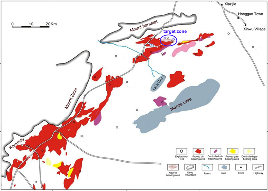
FIGURE 1. Geographical location map of Fengcheng oilfield (adapted from Zhou, 2016).
Geologically, the regional structure of Fengcheng oilfield is located in the Mesozoic overlap pinch out zone on the hanging wall of the Xiahongbei fault in the Wuxia fault fold belt, northwest margin of the Junggar basin. From top to bottom, the formations can be divided into the Cretaceous Tugulu group, Jurassic Qigu formation, Sangonghe formation, Badaowan Formation, Triassic, Permian, and Carboniferous. The Jurassic system is in angular unconformity contact with the overlying and underlying strata, and the upper and lower Jurassic systems are also in angular unconformity contact (Huang et al., 2020). Oil sands in this area mainly develop in shallow strata of Cretaceous Qingshuihe Formation K1q and Jurassic Qigu formation J3q (Huang et al., 2020), and our target strata is located in J3q.
Compared to conventional oil reservoirs, the heavy oil reservoir in Fengcheng oilfield generally locates at shallow depth (several hundred meters). Oil has a density of .96 g/cm3 (API = 16), close to water density, making it difficult to distinguish the oil formations from water formations. Moreover, it has a viscosity over 5 × 10⁵ mPa s (at 20°C) (Huang et al., 2020), increasing the difficulty of production. The high density plus high viscosity also cause troubles for reservoir exploration and production assessment. To better characterize the heavy oil reservoir through seismic methods and to improve the evaluation of drilling risks in production, it requires inspecting the heavy oil sands elastic properties and consolidation status under in situ conditions. However, current methods for characterizing the elastic properties of Fengcheng heavy oil reservoirs mainly involve well logs inspection without rock physics analysis and modeling (Huang et al., 2020); thus, they cannot be integrated with seismic methods effectively, resulting in limited knowledge of the reservoirs in large scales.
This rock physics study is performed to systematically investigate the elastic properties and consolidation status of heavy oil sands in Fengcheng oilfield. Petrophysical analysis of the well logs was firstly conducted to determine the oil sands formations and the corresponding elastic properties. Then, the porosity log was predicted by combining the neutron and density logs, and the velocity differences in different sections were also analyzed. Based on the identified heavy oil formations and laboratory measurement, the heavy oil sands’ velocities were theoretically modeled, and the rocks’ consolidation status was evaluated. Finally, the modeling results of the two nearby wells were compared, and the reasons of the differences were explained.
2 Methodology
The available data include two sets of well logs (from well #1 and well #2 as indicated in the blue circle in Figure 1), laboratory measured porosity and oil saturation of 6 samples (Table 1), and statistical grain sizes of the formations in well #1. The laboratory data are from the measurements in the Applied Petrophysics Lab (APL) in China University of Petroleum (East China).
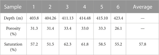
TABLE 1. Measured porosity and oil saturation of the core samples from well #1.
2.1 Well log analysis
The well logs of well #1 include GR, RT, CNL, DTC, DTS, and DEN logs, which are shown in Figure 2.
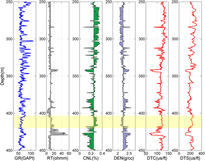
FIGURE 2. Well logs of well #1 from Fengcheng oilfield. GR means gamma ray log; RT means resistivity log; CNL means compensated neutron log; DEN means density log; DTC means compressional wave slowness log; DTS means shear wave slowness log; and the yellow section marks the target zone.
In Figure 2, it can be seen that 342–346 m depth section has relatively low GR, high RT, low CNL, low DTC, low DTS, and high DEN, which means it has low clay content, low porosity, high P-wave velocity (Vp), high S-wave velocity (Vs), and high density. These characteristics suggest that it is impossible to be oil sands; rather, it is more likely to be tight sand or limestone. The 379–383 m section has similar characteristics as the 342–346 m section, except that the GR is higher, suggesting the higher clay content, thus it is probably shale. The 386–392 m depth section has low GR and high RT, and CNL is around 30%. The Vp, Vs, and density are smaller than those of the above and beneath layers. It might be oil sands. The 403–425 m section is featured with low GR, high RT, high CNL, high DTC, high DTS, and low DEN, which are the typical characteristics of oil sands. We conclude it as the oil sands layer, which is also confirmed by the core samples (Table 1). The 426–430 m section is featured with high GR, high RT, low CNL, low DTC, low DTS, and high DEN, suggesting it has high clay content, low porosity, high Vp, high Vs, and high density. It is highly possible that this section is corresponding to a shale layer. Considering that the laboratory measured samples are from the depth of 403–425 m, to better integrate the log data and laboratory measurements, we take this depth section as the target zone (the yellow marked zone in Figure 2). All the following processing and analysis of well #1 are based on this section.
2.2 Porosity estimation
It is essential to first obtain the porosity to characterize the oil sands properties. The porosities of six core samples were measured using mercury intrusion porosimetry, which was conducted in APL, as shown in Table 1. However, to quantitatively analyze the rock properties of the whole depth section, it is necessary to estimate the porosity log. Here, we combine the density log and neutron log to predict the porosity. First, we assume the oil sands are fully saturated (by oil and water). Then, the rock bulk density can be represented as follows:
where ρb is the rock bulk density; ρg, ρo, and ρw are the densities of the grains, oil, and water, respectively. The strata are sand, and so, the grain density is assumed to be 2.65 g/cm3. ϕρ is porosity; So and Sw are the oil and water saturation, respectively; and
In Eq. 1, since the porosity and oil saturation are unknown, it is impossible to invert the porosity with these available data. Considering that the oil density (.96 g/cm3) is close to water density (1.0 g/cm3), we further assume the oil has the same density as water (the uncertainty will be analyzed in the Discussion section), then Eq. 1 can be simplified.
and the porosity can be calculated with the following equation:
Then, following the method of Aliyeva et al. (2012), true porosity ϕ can be estimated by averaging this density-porosity ϕρ and neutron—porosity ϕN (CNL log in Figure 2) in the following equation :
The estimated porosity is compared with the laboratory measured porosity in Figure 3. It can be seen that the CNL-log predicted result evidently overestimates the porosity, while the density-log predicted result underestimates the porosity. Comparatively, the calculated porosity log matches well with the measured core data, demonstrating that the prediction is reliable.
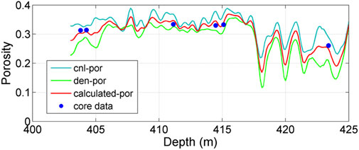
FIGURE 3. Calculated porosity log. The cyan line indicates the CNL-log predicted porosity, the green line indicates the density-log predicted porosity, and the red line indicates the estimated porosity using the current method. It is clear that the estimation matches the laboratory measured data, demonstrating the reliability of the estimation results.
2.3 Velocity analysis
To better understand the relations between the velocities, Vp/Vs ratios, depth, density, and porosity, we plot the scattered data in Figures 4, 5.
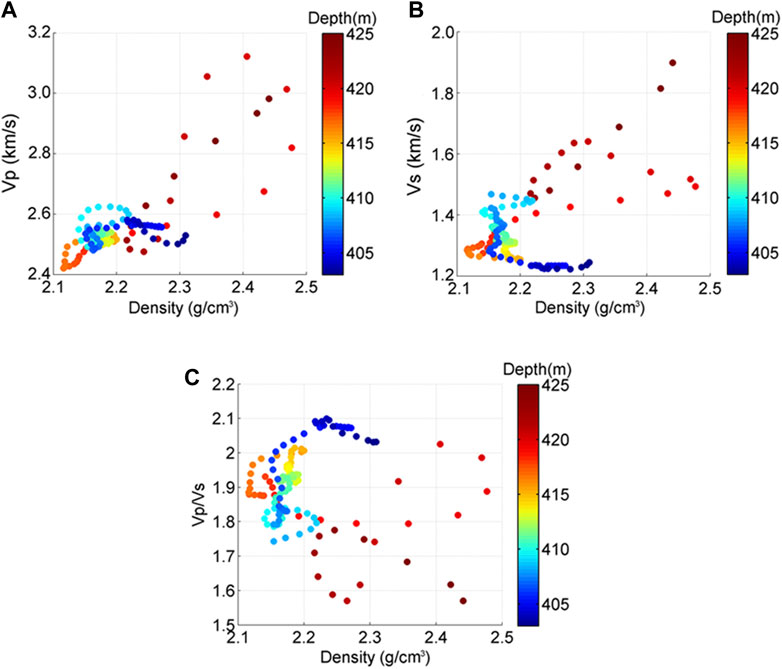
FIGURE 4. Cross-plot of density, depth, and (A) Vp, (B) Vs, and (C) Vp/Vs ratio.
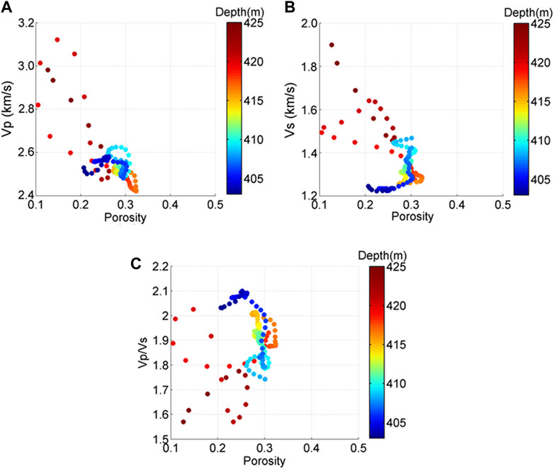
FIGURE 5. Cross-plot of porosity, depth, and (A) Vp, (B) Vs, and (C) Vp/Vs ratio.
In Figure 4, one most evident observation is that the oil sands formation is very shallow, only around 400 m. This depth is much shallower than the conventional oil reservoirs, which are generally buried over one thousand meters. The density is between 2.1 and 2.5 g/cm3, Vp is between 2.4 and 3.1 km/s, and Vs is between 1.2 and 1.9 km/s, relatively smaller than conventional oil-bearing sandstones. In addition, it can be found that the data distribute in two distinct zones: the data of 403–418 m depth section mainly cluster around 2.1–2.3 g/cm3 with Vp of 2.4–2.62 km/s and Vs of 1.2–1.48 km/s; while the data of 418–425 m depth section have relative larger density between 2.3 and 2.5 g/cm3, larger Vp of 2.6–3.1 km/s, and larger Vs of 1.4–1.9 km/s. Considering that the two sections do not have much depth gap, the differences are impossible to be caused by the compaction and pressure; rather, it should be owing to other factors, e.g., matrix heterogeneity. Figure 6 shows the statistical distribution of grain sizes of the sections. It can be observed that the 418–425 m section has more large-size grains (size above .25 mm) and less middle-size grains (.063–.25 mm) than the 403–418 m section. On the other hand, the 403–418 m section has relatively better sorting as its grain sizes focus in a narrower range. These different grain size distributions and sorting can cause heterogeneity of the sand matrix. This is also verified by the porosity log in Figure 3, which shows that the 403–418 m section has relatively larger and stable porosities than the 418–425 m section. Hence, the matrix heterogeneity is a possible reason for the different velocities (more discussion is shown in the Discussion section).

FIGURE 6. Statistical distribution of the grain size.
The oil sands have large porosities (Figure 5), which could go up to .33. In addition, porosity distributes in a wide range between .11 and .33, further justifying the heterogeneity. The Vp/Vs ratios are mostly above 1.75, which are relatively larger than conventional sandstones. In addition, the deep-section sands (418–425 m) have relatively lower porosity, consistent with the porosity log in Figure 3; and their Vp/Vs ratios are smaller compared to the shallow section sands (403–418 m), which can also be attributed to the matrix heterogeneity as explained previously. Overall, most of the data are clustered at Vp of 2.4–2.65 km/s and Vs of 1.2–1.48 km/s, evidently smaller than conventional sandstones.
3 Rock physics modeling
3.1 Fluid mixture modeling
To simulate the oil sands elastic properties, it is essential to know the frame and fluid properties. According to the previous studies in this area (Guo and Han, 2016; Huang et al., 2020), the rock frame is primarily composed of quartz sand grains. Hence, the moduli of the rock matrix can be referred to the moduli of quartz with a bulk modulus of 37 GPa and shear modulus of 45 GPa.
Because heavy oil properties are highly temperature-dependent, it is necessary to figure out the heavy oil properties under in situ conditions. The in situ pressure is around 5 MPa (Guo and Han, 2016). Considering that the surface temperature is around 10°C, the depth is around 400 m, the geothermal gradient is around 25°C/km, and the in situ temperature is approximately 20°C. The density of the fluid mixture can be calculated by the following equation:
where ρR is the effective density of the mixture and fi and ρi are the fraction and density of the ith component, respectively. The calculated mixture density is shown in Figure 7A.
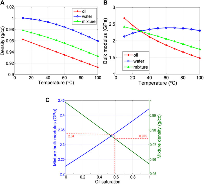
FIGURE 7. Variation of (A) bulk modulus and (B) density of the heavy oil, water, and fluid mixture with temperature. (C) Variation of bulk modulus and density of the fluid mixture with oil saturation. The bulk modulus of the fluid mixture is predicted using Wood’s equation.
According to the prediction of the FLAG program (developed by FLUIDS/DHI consortium of University of Houston and Colorado School of Mines), the bulk modulus of heavy oil and water under different temperatures are presented in Figure 7B (the oil shear modulus is around .038 GPa under the in situ condition, which has negligible influence on the elastic properties of oil sands and, thus, is not presented). It is clear that the bulk modulus of heavy oil decreases quickly with increasing temperature, revealing the high temperature-sensitivity of the oil, which also justifies the popularity of the thermal production method of heavy oil reservoirs (Yuan et al., 2017). Moreover, it can be seen that the bulk modulus of heavy oil and water are 2.46 and 2.25 GPa, respectively, at 20°C. Since the pores are filled with oil and water, it is necessary to figure out the moduli of the fluid mixture, which is assumed under iso-stress condition and can be estimated through the Wood equation (Wood, 1955) given as follows:
where KR is the effective bulk modulus of the mixture and fi and Ki are the fraction and bulk modulus of the ith component, respectively. As shown in Figure 7B, the bulk modulus of the fluid mixture also decreases with increasing temperature, demonstrating the effect of heavy oil in pore fluids; moreover, it is approximately 2.34 GPa at 20°C. Notably, since the water shear modulus is zero, the mixture shear modulus should also be zero according to the Wood equation.
Given that the average saturation is around 58% (Table 1), the predicted mixture density and bulk moduli are .975 g/cm3 and 2.34 GPa, respectively, as shown in Figure 7C. After the effective bulk modulus of the pore fluid mixture is obtained, the moduli of the oil sands can be estimated with theoretical models. In the subsequent section, we choose the Hertz–Mindlin model, Voigt–Reuss-Hill average, and iso-frame model to conduct the simulation, which are effective and commonly used in characterizing rocks’ consolidation status.
3.2 Hertz–Mindlin modeling
The first model we use is the Hertz–Mindlin model, which establishes the relations between rock moduli, porosity, grain contact, and pressure and can be used to predict the elastic properties of precompacted granular rocks (Mindlin, 1949). It has also been used to estimate the frame modulus of heavy oil sands (Lerat et al., 2010). We use this model to calculate the effective moduli of the dry rock frame and then use the Gassmann equation (Gassmann, 1951) to predict the velocities of the fully saturated oil sands. Figure 8 shows the modeling results.
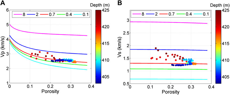
FIGURE 8. Hertz–Mindlin model simulation results of (A) P-wave velocity and (B) S-wave velocity. Different lines indicate simulation results with different coordination numbers. It is clear that most of the data locate around the line with a coordination number of .7.
In Figure 8, the simulation results vary significantly with the coordination number, which describes the number of grain contacts and is an important parameter in the Hertz–Mindlin model. A coordination number of 8, which is a commonly used value for unconsolidated rocks (Hossain et al., 2011), evidently overestimates both Vp and Vs. A coordination number of 1 still overestimates the velocities, while the .4 and .1 coordination numbers underestimate the velocities. The simulation results of .7 coordination number match both Vp and Vs of the data, which indicates that the contacts between the sand grains are quite scarce. This suggests that most of the sand grains are isolated by the pore fluids without much contact and the rock frame is poorly compacted, which is reasonable in light of the shallow depth.
3.3 Voigt–Reuss–Hill (VRH) modeling
To further analyze the rock properties, we also apply the Voigt–Reuss modeling, which describes the iso-strain and iso-stress conditions of the rock components (Hill, 1952), and they are also recognized as the physical upper and lower bounds of the rocks’ moduli. Hill modeling is also applied, which is the average of the Voigt and Reuss bounds and is commonly used to estimate the effective properties of rocks with multiple components (Domenico, 1976; Mavko et al., 2009). This VRH model has also been adopted to analyze oil sands velocities in previous works (Javanbakhti, 2018; Yuan et al., 2020). The modeling results are shown in Figure 9.
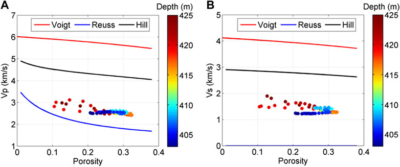
FIGURE 9. VRH simulation results of (A) P-wave velocity and (B) S-wave velocity.
In Figure 9, the data are far below the upper Voigt bound and even below the Hill average. On the other hand, it is close to the Reuss bound, suggesting that most of the components of the oil sands are under iso-stress condition. This further indicates that the sand grains are mostly in the suspension status, which is also consistent with the aforementioned analysis that the grains have few contacts and the frame is poorly consolidated.
3.4 Iso-frame (IF) modeling
The iso-frame model is another effective tool to analyze the rock elastic properties, which is developed by Fabricius (2003). It describes the rock’s elastic properties between the modified upper and lower Hashin–Shtrikman bounds (Hashin and Shtrikman, 1963) and assumes that part of the sand grains are supporting the frame, while the remaining part are in the suspension status (Fabricius, 2003). It can also be used to analyze the rock consolidation status. This model uses an IF parameter to represent the percentage of grains in a load-bearing frame, and thus 1-IF is the percentage of grains in suspension. The modeling results are shown in Figure 10.
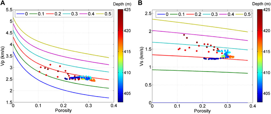
FIGURE 10. Iso-frame model simulation results of (A) P-wave velocity and (B) S-wave velocity. Different lines represent the modeling results with different IF values.
In Figure 10, for Vp, all the data distribute between IF = .1 and IF = .3 with the most gathering around IF = .2. For Vs, most of the data locate between IF = .2 and IF = .4, and the largest cluster is also around IF = .2. Hence, it suggests that approximately 80% of the sand grains are in the suspension status, while only 20% grains are supporting the frame. This further demonstrates that the rock frame is quite loose and poorly consolidated, which is consistent with the aforementioned analysis.
3.5 Modeling results of well #2
Among the abovementioned three models, it seems that compared to the VRH model, the Hertz–Mindlin model and IF model can provide more quantitative assessment of the rock consolidation status (Hertz–Mindlin model with .7 coordination number and IF model with .2 IF value), and they generally match the data better. Hence, we also apply them on the logs of well #2 (Figure 11) to evaluate the consolidation status, which is located near well #1. The simulated sections are the sections of 77.6–86.1, 89.2–95.5, 99.1–102.1, and 104.0–124.4 m. These sections show low GR, high RT, high CNL, low DEN, and high DTC logs, and thus are assumed oil sands formations. Since well #2 does not include the S-wave velocity log, we only show the modeling results of the P-wave velocity. The modeling results are shown in Figure 12.

FIGURE 11. Well logs of well #2. Note that this well does not include the S-wave velocity log.
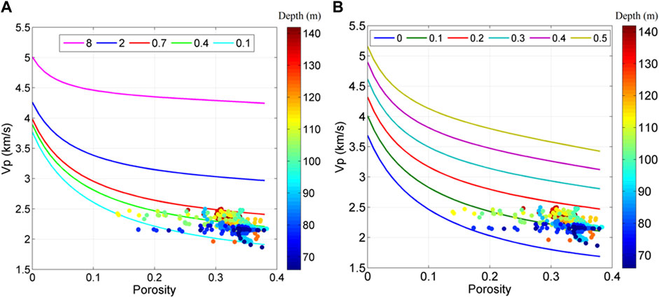
FIGURE 12. Simulated P-wave velocities with (A)the Hertz–Mindlin model and (B) iso-frame model.
In the Hertz–Mindlin modeling in Figure 12A, most of the data distribute around the curve of .4 coordination number, indicating that the average grain contact is around .4. In the IF modeling in Figure 12B, the data mainly cluster around the curve of .1 IF value, suggesting that only about 10% sand grains are supporting the load-bearing frame, while the remaining 90% are in the suspension status. These simulation results both demonstrate that the sand grains are barely, connected and the oil sands are poorly consolidated.
4 Discussion
The oil sands layers are generally featured with large porosity, low Vp, and low Vs, and since the rock matrix is mainly composed of quartz sands, the GR log is of low value. In well #1, we use 403–425 m as the target oil sands section, which does not rule out the possibility of the other sections. For instance, the sections of 350–370 and 386–392 m also show some characteristics of oil sands formation. We use the 403–425 m section because in this section we have laboratory-measured core samples that can confirm the oil presence and also can combine with the section of logs to jointly characterize the oil sands properties. In well #2, we did not perform detailed analysis of the section and assumed the 77.6–86.1, 89.2–95.5, 99.1–102.1, and 104.0–124.4 m sections as the oil sands formations since they have similar characteristics with the oil sands formation in well #1. Moreover, all the data are concentrated in narrow ranges in Figure 12, suggesting that even only a few sections are oil sands layers; they still cluster around the simulation results.
In porosity estimation, the oil density is assumed the same as water density (1.0 g/cm3), which can introduce uncertainty. To analyze the uncertainty, we replace the water with oil completely and then calculate the changes. Then, Eq. 3 changes to the following equation:
Also, the relative error can be obtained through the following equation:
In addition, if according to Table 1, the oil saturation is 58%, then the density of fluid mixture ρm is
and the corresponding uncertainty is
Both the two cases have very small uncertainties. To visually inspect the uncertainties, we plot them in Figure 13. It is clear that the uncertainties are so small that the predicted porosity logs almost overlap each other, which justifies that the assumption of the same density of oil and water leads to trivial uncertainty and has ignorable influence on the estimated porosity.
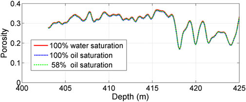
FIGURE 13. Predicted porosity logs under the cases of different oil saturations.
The section of 418–425 m has relatively higher velocities than the section of 403–418 m. Considering that these two sections only have around a 20 m depth gap with up to 5% pressure difference, the pressure and compaction effect cannot be the reason. Instead, it is more possibly to be caused by the matrix heterogeneity induced by the grain size distribution pattern. As illustrated in Figure 6, the deep section (418–425 m) has more large-size grains, while the shallow section (403–418 m) has better sorting with relatively narrower-ranged grain sizes. According to the measurements and analysis of Han et al. (2007), the heavy oil sands with larger grain sizes tend to have larger velocities, and the oil sands with better sorting tend to have smaller velocities. Hence, the grain size distribution and sorting caused matrix heterogeneity, which is also confirmed by the porosity log in Figure 3, appears as a possible reason for the velocity difference of the two sections.
Due to the lack of XRD/thin section analysis of the core samples, detailed mineral components of the matrix are unknown. However, based on the previous studies conducted in the same area (Guo and Han, 2016; Huang et al., 2020), the matrix is mainly composed of quartz sand grains. Hence, we also assume the pure quartz sand matrix. On the other hand, however, if the matrix contains clay which has smaller bulk modulus, shear modulus, and density than quartz, then the matrix density and moduli would both be smaller. In such case, the predicted porosity would be larger, and the predicted velocities would be smaller than the current values.
A lot of rock physics models are available for simulating oil sands elastic properties (Guo and Han, 2016; Yuan et al., 2020; Qi et al., 2021; Zhang et al., 2021; Zhang et al., 2022). However, only three models (Hertz–Mindlin model, Voigt–Reuss–Hill average, and iso-frame model) are used here, mainly due to two reasons. First of all, the target of the study is to evaluate the consolidation status of the oil sands, and these three models can best serve the purpose through the associated parameters (coordination number in the Hertz–Mindlin model, closeness to Reuss bound in the VRH model, and IF value in the iso-frame model). In particular, the Hertz–Mindlin model and iso-frame model can provide the quantitative assessment of the consolidation status (e.g., coordination number = .7 in the Hertz–Mindlin model and IF = .2 in the iso-frame model). Moreover, these models have also been adopted to simulate the elastic properties of oil sands before (Lerat et al., 2010; Wolf, 2010; Yuan et al., 2020), suggesting that they are suitable for oil sands modeling. Hence, considering the aforementioned two factors, we choose these models to simulate the oil sands.
In the modeling process, a constant oil saturation of 58% is used, which is derived from the average value in Table 1. However, the true oil saturation based on the core measurement varies from 51.5% to 62.3%. To further inspect the influence of saturation variation, the associated bulk modulus and density are picked in Figure 7C, which can be used to calculate uncertainties, as shown in Table 2. It is clear that the uncertainties of the bulk modulus and density of the fluid mixture caused by saturation variation are quite small (bulk modulus uncertainty is below .7%, and density uncertainty is below .3%).
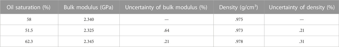
TABLE 2. Uncertainties of the fluid mixture bulk modulus and density. The uncertainties are calculated by comparing the modulus and density values with the values at 58% saturation.
Given that the pore fluids consist of heavy oil and water (oil saturation is around 58%, and water saturation is around 42%), they are assumed under iso-stress condition, and the Wood equation is adopted for pore fluids mixing. Hence, the shear modulus of the fluids mixture is zero. However, the heavy oil under in situ condition is at a semisolid state with a shear modulus (Trippetta and Geremia, 2019), which is around .038 GPa as predicted by the FLAG program. This viscous oil might choke the pore throats and reduce pore connectivity, resulting in patchy distribution of the pore fluids. In such case, the pore fluids are under iso-strain condition, which is more appropriate to simulate with Voigt bound (Mavko et al., 2009). Thus, the corresponding shear and bulk moduli of the fluids mixture would be .022 and 2.35 GPa, respectively, which, however, is not much different from the current value using the Wood equation (2.34 GPa). Therefore, it can be inferred that the fluids mixing with Voigt bound could have some influences on the modeling results, but the differences cannot be significant.
The simulation results of the VRH model and IF model both suggest that the oil sands’ frame is very loose. The Hertz–Mindlin model results directly demonstrate that the grain contacts are quite scarce and most of the grains are in the suspension status, further justifying the poorly consolidated rock frame. These aforementioned results are consistent with the laboratory SEM observations in Figure 14. It is evident that the grains are separated without much contact between them, which justifies that the oil sands are poorly consolidated.
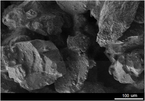
FIGURE 14. The SEM image of oil sands from Fengcheng oilfield.
On the other hand, however, even all the aforementioned models reach the same conclusion of loose frame and rarely-connected grains, the grains are not completely isolated, and the frame does have some consolidation. In the Hertz–Mindin modeling result, the coordination number is around .7, meaning that the average grain contact is .7, which, although small, is still above 0. In the VRH modeling result, the data distributes close to Reuss bound, but there is still some gap between them. This gap is because the grains are not completely separated, and there are still some grain contacts remaining. In the IF modeling, although the results suggest that 80% of the grains are in suspension, there are still 20% remaining in the load-bearing frame.
Comparing Figures 8, 10, 12, it can be found that well #2 has a smaller coordination number and IF value than well #1, which suggests that the rock frame of oil sands in well #2 is weaker than that in well #1. We think there are three possible reasons. The first one is that the formations in #2 are shallower than in #1 (100 m compared to 400 m). The shallower depth means smaller overburden pressure, and thus the rock frame is less compacted than that in well #1. Under this condition, the simulation results have no problem and correctly reveal the consolidation status of these formations in well #2. The second reason is related to the clay content. By comparing Figures 2, 11, it can be found that well #2 has higher values of GR log than well #1, which indicates it has higher clay content. This higher clay content makes the true rock matrix “softer” with smaller moduli, and thus the simulation results using the (default) quartz mineral matrix overestimate the velocities, leading to the conclusion of relatively weaker oil sands in well #2. A third possible reason is about the oil saturation. In well #1, the saturation is around 58% (according to Table 1). However, if the saturation of the oil sands in well #2 is lower than 58%, then according to Eq. 6, the true bulk modulus of the fluids mixture will be smaller than 2.34 GPa, resulting in an overestimation of the simulation results which uses 2.34 GPa as the bulk modulus of fluids mixture. Given that the formations in well #2 are shallower than in well #1, this is also a reasonable and possible explanation.
Overall, even though there are differences between the estimated parameters of the Hertz–Mindlin model and IF model in wells #1 and #2, the differences are small and they both demonstrate that the oil sands in this area are loose and poorly consolidated, which can provide useful information for seismic characterization and production evaluation of the oil sands reservoirs in this oilfield.
5 Conclusion
The heavy oil sands in Fengcheng oilfield are located at shallow depth with Vp between 2.4 and 3.1 km/s and Vs between 1.2 and 1.9 km/s. The porosities are mostly between .2 and .4, and the average oil saturation obtained from the laboratory measurement is around 58%.
The predicted porosity through combining the density log and neutron log matches well with the laboratory measured sample porosities, demonstrating the effectiveness of the method. The grain size distribution and different sorting lead to the matrix heterogeneities, which further cause the different velocities of the shallow section (403–418 m) and deep section (418–425 m) in well #1. The theoretical modeling demonstrates that the rock velocities are generally at low level. The results suggest that the grain contacts are scarce, and the frame is loose and poorly consolidated, which are consistent with the SEM observations. Overall, this study demonstrates that the integration of well log, laboratory data, and rock physics models works effectively in analyzing the consolidation status of the heavy oil sands, which can provide valuable implications for seismic characterization and drilling risk evaluation.
Data availability statement
The original contributions presented in the study are included in the article/Supplementary Material; further inquiries can be directed to the corresponding author.
Author contributions
HY: conceptualization, methodology, funding acquisition, and writing—original draft. XH: conceptualization and data acquisition. XZ: writing—revising draft and project administration. YW: writing—revising draft.
Funding
This research was supported by the National Natural Science Foundation of China (Grant 42104118, U1839208, and 41804132) and New Teacher Research Ability Improvement Project in China University of Geosciences (Beijing).
Acknowledgments
The authors are grateful to the colleagues in China University of Geosciences (Beijing) for support and discussion.
Conflict of interest
The authors declare that the research was conducted in the absence of any commercial or financial relationships that could be construed as a potential conflict of interest.
Publisher’s note
All claims expressed in this article are solely those of the authors and do not necessarily represent those of their affiliated organizations, or those of the publisher, the editors, and the reviewers. Any product that may be evaluated in this article, or claim that may be made by its manufacturer, is not guaranteed or endorsed by the publisher.
References
Aliyeva, S., Dvorkin, J., and Zhang, W. (2012). Oil sands: Rock physics analysis from well data, alberta, Canada. Las Vegas, NV: SEG Tech. Program Expanded Abstr, 1–5.
Domenico, S. N. (1976). Effect of brine-gas mixture on velocity in an unconsolidated sand reservoir. Geophysics 41, 882–894. doi:10.1190/1.1440670
Fabricius, I. L. (2003). How burial diagenesis of chalk sediments controls sonic velocity and porosity. AAPG Bull. 87, 1755–1778. doi:10.1306/06230301113
Gassmann, F. (1951). Elastic waves through a packing of spheres. Geophysics 16, 673–685. doi:10.1190/1.1437718
Guo, J., and Han, X. (2016). Rock physics modelling of acoustic velocities for heavy oil sand. J. Petrol. Sci. Eng. 145, 436–443. doi:10.1016/j.petrol.2016.05.028
Han, D. H., Yao, Q. L., and Zhao, H. Z. (2007). Complex properties of heavy oil sand. Seg. Tech. Program Expand. Abstr., 1605. doi:10.1190/1.2792803
Hashin, Z., and Shtrikman, S. (1963). A variational approach to the theory of the elastic behaviour of multiphase materials. J. Mech. Phys. Solids. 11, 127–140. doi:10.1016/0022-5096(63)90060-7
Hill, R. T. (1952). On discontinuous plastic states, with special reference to localized necking in thin sheets. J. Mech. Phys. Solid 1, 19–30. doi:10.1016/0022-5096(52)90003-3
Hossain, Z., Mukerji, T., Dvorkin, J., and Fabricius, I. L. (2011). Rock physics model of glauconitic greensand from the North Sea. Geophysics 76 (6), E199–E209. doi:10.1190/geo2010-0366.1
Huang, W., Wang, X., Sun, X., Xie, Z., Zhou, B., Xiong, W., et al. (2020). Exploration and production practice of oil sands in Fengcheng oilfield of Junggar Basin, China. J. Pet. Explor Prod. Technol. 10, 1277–1287. doi:10.1007/s13202-019-00828-w
Javanbakhti, A. R. (2018). Empirical modeling of the saturated shear modulus in heavy oil saturated rocks. Calgary, AB: Ph.D. Dissertation, University of Calgary.
Lerat, O., Adjemian, F., Baroni, A., Etienne, G., Renard, G., Bathellier, F., et al. (2010). Modelling of 4D seismic Data for the monitoring of steam chamber growth during the SAGD process. J. Can. Petrol.Technol. 49, 21–30. doi:10.2118/138401-pa
Mavko, G., Mukerji, T., and Dvorkin, J. (2009). The rock physics handbook: Tools for seismic analysis in porous cambridge. London, UK: Cambridge University Press.
Meyer, R., and Attanasi, E. (2003). Heavy oil and natural bitumen- strategic Petroleum resources. Reston, VA: U.S. Geological Survey.
Mindlin, R. D. (1949). Compliance of elastic bodies in contact. J. Appl. Mech. 16, 259–268. doi:10.1115/1.4009973
Qi, H., Ba, J., Carcione, J. M., and Zhang, L. (2021). Temperature-dependent wave velocities of heavy oil-saturated rocks. Lithosphere 3, 3018678. doi:10.2113/2022/3018678
Trippetta, F., and Geremia, D. (2019). The seismic signature of heavy oil on carbonate reservoir through laboratory experiments and AVA modelling. J. Petrol Sci. Eng. 177, 849–860. doi:10.1016/j.petrol.2019.03.002
Wolf, K. (2010). Laboratory measurements and reservoir monitoring of bitumen sand reservoirs. Stanford, CA: Stanford University.
Yuan, H., Han, D. H., Li, H., and Zhang, W. (2020). The effect of rock frame on elastic properties of bitumen sands. J. Petrol Sci. Eng. 194, 107460. doi:10.1016/j.petrol.2020.107460
Yuan, H., Han, D. H., and Zhang, W. (2017). Seismic characterization of heavy oil reservoir during thermal production: A case study. Geophysics 82 (1), B13–B27. doi:10.1190/geo2016-0155.1
Zhang, L., Ba, J., and Carcione, J. M. (2021). Wave propagation in infinituple-porosity media. J. Geophys. Res. Solid Earth. 126 (4), e2020JB021266. doi:10.1029/2020jb021266
Zhang, L., Ba, J., Carcione, J. M., and Wu, C. (2022). Seismic wave propagation in partially saturated rocks with a fractal distribution of fluid-patch size. J. Geophys. Res. Solid Earth. 127 (2), e2021JB023809. doi:10.1029/2021jb023809
Zhang, S., Zhang, Y., Wu, S., Liu, S., Li, X., and Li, S. (2005). “Status of heavy oil development in China,” in SPE International Thermal Operations and Heavy Oil Symposium, Calgary, Alberta, Canada, November 1–3, 2005. SPE-97844-MS.
Keywords: heavy oil sands, consolidation status, rock physics modeling, acoustic velocity, unconventional reservoir
Citation: Yuan H, Han X, Zhang X and Wang Y (2023) Evaluation of the consolidation status of heavy oil sands through rock physics analysis: A case study from Fengcheng oilfield. Front. Earth Sci. 10:1103321. doi: 10.3389/feart.2022.1103321
Received: 20 November 2022; Accepted: 21 December 2022;
Published: 06 January 2023.
Edited by:
Qiaomu Qi, Chengdu University of Technology, ChinaCopyright © 2023 Yuan, Han, Zhang and Wang. This is an open-access article distributed under the terms of the Creative Commons Attribution License (CC BY). The use, distribution or reproduction in other forums is permitted, provided the original author(s) and the copyright owner(s) are credited and that the original publication in this journal is cited, in accordance with accepted academic practice. No use, distribution or reproduction is permitted which does not comply with these terms.
*Correspondence: Hemin Yuan, yhm3414@gmail.com