Studies of natural gas production prediction and risk assessment for tight gas in Sichuan Basin

After a new round of tight gas geological evaluation was launched in 2018, a new chapter of tight gas exploration and development has been opened in the Sichuan Basin. In order to make better planning work, it is very important to study the variation rule and risk assessment of tight gas production. In this paper, the peak production is predicted by Ward model. Based on the prediction results, Hubbert and Gauss models were established to study the variation law of tight gas production, and the accuracy and prediction results of the models were determined by the degree of fitting and correlation coefficient. By studying the relationship between URR and production, it is concluded that the production increases in a step, and the future production of tight gas is simulated from the perspective of realization probability. Finally, the risk assessment matrix is established to study the difficulty degree of achieving the production target. The results are as follows: 1) Hubbert model has higher accuracy in predicting tight gas production change. The peak year of tight gas is 2042, the peak production is $\left(86-106\right)\times {{10}^{8}m}^3/\mathrm{a}$, and the final URR recovery degree is about 60%. 2) The realization probability of production is calculated, and the possibility of reaching the target value is evaluated from the perspective of risk, so as to guide the production of tight gas, and finally promote the formulation of tight gas development planning in the Sichuan Basin.

1 Introduction

The breakthroughs made by the natural gas industry have improved the energy structure and promoted the development of a low-carbon economy. Current international development trend is basically green energy, advocating energy saving and carbon reduction, the oil and gas field has turned to natural gas as the focus. Therefore, the efficient development of natural gas is extremely important (Chengzao et al., 2014; Jia, 2018). In natural gas development planning, it is necessary to carry out peak production prediction and risk quantitative analysis. Through peak production prediction and risk quantitative analysis, a judgment mechanism that is coordinated with accuracy and rationality is formed, so as to achieve the purpose of optimizing development benefits. Only by establishing a prediction method that accurately describes the law of production growth and reasonably predicting the change trend of natural gas production can the basin exploration planning work be better formulated, and risk quantification research can be carried out based on the production prediction results (WANG et al., 2016; TONG et al., 2018).

In recent years, the exploration potential of tight gas has been explored and gradually been paid attention to, becoming a new force of natural gas in our country, with large-scale production in Sichuan, Ordos, Songliao and other basins, and has become a key area for increasing oil and gas reserves and production in China. In order to continue to promote the exploration and development of tight gas in the Sichuan Basin, a new round of evaluation of tight gas geological conditions was launched in 2018. The Jinhua-Qilin area in central Sichuan was selected as a pilot area for the integration of tight gas exploration and development, and technical research and management model innovation were carried out. Especially in 2020, the tight gas resource potential of the Sichuan Basin was re-evaluated, and the central Sichuan area was selected as the core production area for tight gas. New drilling and testing of natural gas production have repeatedly hit new highs, opening a new chapter for tight gas exploration and development in the Sichuan Basin (Wu. et al., 2021; Huang. et al., 2022). The development of tight gas in the Sichuan Basin is still in the early stage of exploration, and the proved rate is even less than 20%. There is a huge amount of tight gas exploration, and it is also the focus of development in the Sichuan Basin in the future, which plays a crucial role in the development of natural gas production and economy (DAI et al., 2021; Lin et al., 2021).

However, tight gas reservoirs have the characteristics of strong heterogeneity, small pore size, low permeability, and strong stress sensitivity, which require fracturing development. The particularity of reservoirs, fluid seepage characteristics and the multiple complexity of fracturing stimulation measures make it difficult to predict the productivity of tight gas, it is difficult to obtain the variation law of tight gas production and the actual production value that can be achieved (Zheng et al., 2021). Therefore, it is necessary to predict the growth trend of tight gas production in this area, analyze the realization probability of its peak production, and guide the planning of tight gas based on production prediction and risk assessment.

At present, there are many researches on natural gas production prediction models, such as peak prediction method, grey system method, neural network method, etc (Mohr and Evans, 2011; Zeng. et al., 2020). Comparing these methods, it can be seen that the peak prediction method is more suitable for the study of production variation law (Zheng et al., 2020). For natural gas fields that are still in the early stage of development or production, the peak prediction method is more accurate and more practical for medium and long-term prediction (Ravnik et al., 2021; Wang. et al., 2022). Lao. and Sun. (2022) combined with the dispersion coefficient, established the Bernoulli model with nonlinear distribution, which is also the representative model of grey prediction. The model can accurately analyze those predictions to a certain extent. Finally, the model is used to prediction natural gas consumption and production in China, and corresponding suggestions are given based on the prediction results. The Hubbert model established by Sun et al. (2021) can better predict the change of production, and this model has multiple life cycles, and URR is introduced to participate in the prediction of production. Then, through grey relational analysis, the best consumption curve corresponding to different URR scenarios is selected. Empirical results show that natural gas production of China cannot meet the growing consumption. Therefore, policy measures must be taken to alleviate this situation. Accurate prediction of natural gas production and consumption can inform decision-making and help governments formulate new major policies. Wang et al. (2018) introduced the ultimate recoverable reserves as a boundary condition into the multi-cycle Gauss model to predict the trend of natural gas production (Guo et al., 2021). JamesWard. et al. (2012) used a newly developed model to prediction growth in fossil fuel production. The prediction of the Ward model only needs to combine the production data in recent years and the historical cumulative production. This prediction method is worthy of reference.

At present, there are many research methods for risk quantification of natural gas reserves and production, including probability method, neural network method, fuzzy clustering method, etc (Ward et al., 2018; Yiping et al., 2021). Compared with these methods, it can be seen that the probability method is more suitable for risk assessment, especially for the calculation of the risk level of tight gas in the Sichuan Basin. Probabilistic method can be used to determine the degree of difficulty to achieve the target production, so as to guide the planning of exploration and development. Based on the generalized Weng’s model commonly used in the life cycle model method, Chong et al. (2021) established an improved multi-cycle generalized Weng’s model to determine the number of cycles in oil and gas field production prediction, so as to improve the prediction effect of the model. The improved model is applied to the production prediction of Daqing Oilfield, and it is fitting effect on annual production is obviously better than that of the single-cycle model and the multi-cycle model. Shih-Chi et al. (2005) combined a Bayesian approach with a Monte Carlo approach to quantify and update uncertainty in life cycle assessment results. Flouri et al. (2015) investigated how gas supply disruptions in Algeria, the EU’s third-largest supplier, affect gas security in Europe. Using Monte Carlo simulations, results were analyzed for the most affected countries, emphasizing the importance of supply diversification, reserves and production to enhance gas security.

In order to develop a better tight gas planning scheme, production targets should be studied from multiple perspectives. Among them, it is very important to predict the change rule and peak range of production, calculate the realization probability of target production, and evaluate the risk of production. This paper is based on the actual situation of tight gas core production areas in central Sichuan. First, the Ward model was used to predict the peak production and peak year, and then the ultimate recoverable reserves URR was introduced into the Hubbert and Gauss prediction model as a boundary condition. The accuracy of the two prediction models was compared and analyzed, and the production prediction results of tight gas in the Sichuan Basin were obtained. Then, according to the principle of Monte Carlo method, the realization probability of production in different stages is calculated and analyzed, and compared with the change rule of peak production and model parameters with URR, and the risk assessment of target production in different stages is carried out combined with the degree of dispersion. Through the self-built production grade evaluation matrix, a systematic quantitative research on the production risk of natural gas is carried out. The Figure 1 shows the flow chart of the research work.

FIGURE 1

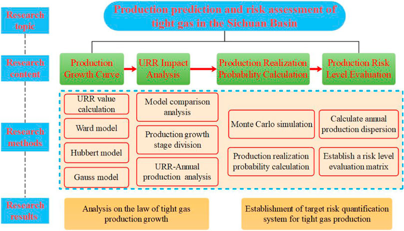
FIGURE 1. Flow chart of tight gas production prediction and risk assessment.

2 Tight gas production prediction and risk quantification theory

2.1 Tight gas production prediction theory

2.1.1 Ward predictive model

Tight gas is currently in the initial stage of development, especially in the core production area of tight gas in Sichuan, where production data is scarce and cannot be fitted with conventional prediction models. Therefore, this paper adopts Ward’s research idea (JamesWard. et al., 2012), takes URR as the qualification, and predicts the future production results according to the specified initial growth rate. The production value of a certain year is used as the initial production for the start of the growth curve, that is, at the beginning of the prediction, an initial production value is specified, and then the trend of production change is studied and the peak production is estimated. The Ward model equations are as follows.

$Q=Q_0{e}^{kt}\left(1-\frac{Q\left(t\right)}{\mathit{U}\mathit{R}\mathit{R}}\right).(1)$

In the formula, $Q$ is the annual production, the unit is ${{10}^{8}m}^3/\mathrm{a}$; $Q_0$ is the initial production; $k$ is the growth rate; t is the time; $Q\left(t\right)$ is the annual cumulative production;URR is the ultimate recoverable reserves.

The Ward predictive model is an asymmetric growth curve of production from a given point, which is a left-biased curve. Compared with the symmetrical curve and the right-biased curve, the left-biased curve allows the production to maintain a longer production growth period and a higher peak production. Therefore, tight gas can be developed as quickly as possible, and the driving effect of tight gas on total natural gas production can be maximized.

2.1.2 Hubbert predictive model

Hubbert model is very suitable for the study of tight gas production trend. After the production of a gas field starts, the production will increase continuously with the increase of time. After experiencing the rapid growth stage and slow growth stage, the production begins to stabilize and reach a stable period, and then the production begins to decline. And the area between the production curve and the time axis is equal to the ultimate recoverable reserves URR (Tilton, 2018). The Hubbert model equations are as follows (Guo et al., 2021).

$P=\frac{\mathit{U}\mathit{R}\mathit{R}}{1+e^{-b\left(t-t_m\right)}}.(2)$

In the formula, $P$ represents the cumulative production, the unit is ${{10}^{8}m}^3/\mathrm{a}$; $\mathit{U}\mathit{R}\mathit{R}$ is the ultimate recoverable reserve, the unit is ${10}^8{m}^3$; $t$ is the production mining time; $t_m$ is the production peak time; $b$ is the model parameter.

Equation 2 can be derived from t to get the formula for calculating annual production:

$Q=\frac{dP}{dt}=\frac{b\times \mathit{U}\mathit{R}\mathit{R}\times e^{-b\left(t-t_m\right)}}{{\left[1+e^{-b\left(t-t_m\right)}\right]}^2}.(3)$

In the formula, $Q$ represents the annual production, the unit is ${{10}^{8}m}^3/\mathrm{a}$.

When $t=t_m$, the production growth peaks. At this time, the rate of change of the cumulative production $P$ is the largest, that is, the $dP/dt$ is the largest. At this time:

$Q_m=b\times \frac{\mathit{U}\mathit{R}\mathit{R}}{4}.(4)$

In the formula, $Q_m$ is the peak annual production, the unit is ${{10}^{8}m}^3/\mathrm{a}$.

Transform Eq. 4 into $\mathit{U}\mathit{R}\mathit{R}=4Q_m/b$, and substitute it into Eq. 3. The annual production calculation formula of the Hubbert model can be obtained (Wang et al., 2016).

$Q=\frac{2Q_m}{1+\mathit{cosh}\left[b\left(t-t_m\right)\right]}(5)$

The curve trend predicted by using the Hubbert model is a gradual increase, and changes from a rapid increase to a slow increase, forming a stable phase around the peak production, and then gradually decreasing.

2.1.3 Gauss predictive model

Gauss model is also suitable for tight gas production prediction. The change trend curve is usually slighter and taller when Gauss model is used for prediction, but the overall change trend is consistent with Hubbert model from a macro perspective, and both of them are symmetrical with the peak yield as the axis of symmetry. Therefore, two models should be used in the study and the more accurate model should be selected (Hu et al., 2020; Luz-Sant’Ana. Patricia Roman-Roman. et al., 2017). The Gauss model equations are as follows.

$f\left(t\right)=\frac{1}{s\sqrt{2\pi }}{e}^{-{\left(t-\mu \right)}^2/2s^2}(6)$

In the formula, $\mu$ is the mean; $s$ is the standard deviation.

In the process of tight gas mining, the cumulative production of mining time in the interval $\left(0-\infty \right)$ is regarded as the ultimate recoverable reserves (URR). Multiply the distribution density function $f\left(t\right)$ by the ultimate recoverable reserves to obtain the formula for calculating the annual production $Q$ (Zhang and Zhao, 2021).

$Q=\frac{URR}{s\sqrt{2\pi }}{e}^{-{\left(t-\mu \right)}^2/2s^2}(7)$

Eq. 7 is derived with respect to the mining time.

$\frac{dQ}{dt}=\frac{\mathit{U}\mathit{R}\mathit{R}}{s\sqrt{2\pi }}{e}^{-{\left(t-\mu \right)}^2/2s^2}\left(-\frac{t-\mu }{s^2}\right)(8)$

When the production change reaches its highest value, annual rate of change in production is $dQ/dt=0$. At this time, the peak time of annual production.

$t_m=\mu (9)$

Substitute $t_m=\mu$ into Eq. 7 to obtain the peak annual production $Q_m$.

$Q_m=\frac{\mathit{U}\mathit{R}\mathit{R}}{s\sqrt{2\pi }}.(10)$

Substituting Eqs 9, 10 into Eq. 7, the annual production calculation formula of the Gauss model can be obtained.

$Q=Q_m{e}^{-{\left(t-t_m\right)}^2/2s^2}.(11)$

In the formula, the model parameter $s$ can characterize the fluctuation of the peak to a certain extent.

2.2 Production risk quantification theory

2.2.1 Monte Carlo probability method

Monte Carlo probability method is based on probability theory and mathematical statistics theory. The basic idea of this method is to establish a probability calculation model, and then obtain the statistical characteristics of the probability through sampling experiments, so as to obtain the approximate result of the realization probability. Monte Carlo method can describe the characteristics of things with random nature more realistically, and it is less limited in calculation. Therefore, this method is suitable for the probability estimation of production and plays an important role in the risk assessment of production in this paper.

When estimating the production probability according to the principle of Monte Carlo method, the problem to be solved should be transformed into the expected value of a probability model, and then the model should be randomly sampled. Finally, a simulation experiment is carried out on the computer, enough random numbers are drawn and statistical analysis is carried out on the problem to be solved (Krupenev. et al., 2020).

Assuming that the distribution density of the known random variable $f\left(x\right)$ is $\psi \left(x\right)$, the mathematical expectation of the variable $f\left(x\right)$ is:

$E={{\displaystyle \int }}_{x_0}^{x_1}f\left(x\right)\psi \left(x\right)\mathrm{d}x.(12)$

According to the distribution density function $\psi \left(x\right)$, N sample points $x_i$ are randomly selected, and the arithmetic mean value of the function value $f\left(x_i\right)$ corresponding to the sample points is used as the integral estimation value.

$\overline{E_N}=\frac{1}{N}{\displaystyle \sum }_{i=1}^{N}f\left(x_i\right).(13)$

According to the probability distribution density function of the variable, the variable values are randomly selected in turn, and the probability density distribution of the objective function can be obtained after a large number of repeated independent simulations of the variable values. Monte Carlo simulation can realize the calculation process of random sampling of variables (Gabriel et al., 2021).

The premise of applying Monte Carlo simulation is to determine the mathematical model of the objective function and the probability distribution of the variables in the model. Each parameter generates a large number of random sample points according to the given probability distribution, which is substituted into the model to calculate the probability density distribution curve of the objective function. The specific steps are shown in Figure 2.

FIGURE 2

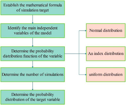
FIGURE 2. Specific steps of Monte Carlo simulation method.

2.2.2 Risk level evaluation matrix

Assessing the risk level of production requires two indicators, the realization probability $P$ and the degree of dispersion of production $C$. The dispersion degree of production represents the degree of difference between a certain production and other production values, that is, the corresponding production value will also change due to the change of risk. The degree of dispersion also indicates the degree of stability of production, that is, the smaller the degree of dispersion of production, the higher its stability (Gutierrez et al., 2016).

The formula for calculating the degree of dispersion is as follows.

$C=1-\frac{\mu }{s}.(14)$

In the formula, $\mu$ is the mean and $s$ is the standard deviation.

Taking into account the two evaluation indicators of production realization probability $P$ and dispersion degree $C$, a risk assessment matrix is established. The production risk is divided into four levels (Figure 3), and the production risk can be comprehensively quantified according to the tight gas production prediction results.

FIGURE 3

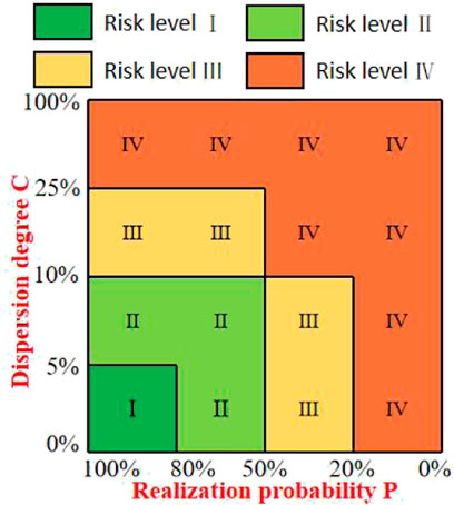
FIGURE 3. Quantitative matrix of production risk level.

The division of the production risk level is mainly determined by the dispersion degree and the realization probability, which is determined by the specific situation of tight gas production. The probability of 80%, 50% and 20% is the most meaningful for the planning. Therefore, these three probabilities are selected as the standard, and the dispersion degree is also divided according to the actual calculation results. The relationship between the grade division principle of risk assessment of production and its corresponding risk matrix is as follows (Guo et al., 2022):

Risk Level I (dark green area in Figure 3): Production targets are very easy to achieve. Division principle: the probability of production realization is $P>80\%$, and the degree of dispersion $C\le 5\%$.

Risk Level II (light green area in Figure 3): Production targets are easy to achieve. Division principle: the probability of production realization is $50\%\le P\le 80\%$, and the degree of dispersion is $C\le 10\%$; or the probability of production realization is $P>80\%$, and the degree of dispersion is $5\%<C\le 10\%$.

Risk Level III (yellow area in Figure 3): Production targets are relatively easy to achieve. Division principle: the probability of production realization is $20\%\le P<50\%$, and the degree of dispersion is $C\le 10\%$; or the probability of production realization is $P>50\%$, and the degree of dispersion is $10\%<C\le 25\%$.

Risk Level IV (orange area in Figure 3): Production targets are not easy to achieve. Division principle: the probability of production realization is $P<20\%$; or the probability of production realization is $20\%\le P<50\%$, and the degree of dispersion is $C>10\%$; or the degree of dispersion is $C>25\%$.

3 Tight gas production prediction

3.1 Estimation of URR and peak production

The production curve of tight gas started in 1964 (Figure 4). The fitting curve of tight gas production maintains a trend of increasing first and then decreasing, and the increasing and decreasing periods are almost symmetrical about the peak value. This is consistent with the prediction curves of the Hubbert and Gauss models, and therefore, the study of tight gas production trend can refer to these two models.

FIGURE 4

FIGURE 4. Fitting curve of tight gas historical production.

As can be seen from the curve, one cycle of mining work has been completed from 1964 to 2020. However, in 2020, the potential of tight gas resources in the Sichuan Basin was re-evaluated, and the central Sichuan area was selected as the core production area for further exploration. At this time, only the production in 2021 and the historical production of the previous cycle are used as a reference. Therefore, the Ward model is used to predict the production peak and peak year of tight gas, and then the models are established to predict the change trend of tight gas production.

Before carrying out tight gas production predestining work, it is necessary to first estimate the numerical range of the ultimate recoverable reserves URR. Through geological exploration, it is found that the current resource of tight gas in the Sichuan Basin is $6.9\times {10}^{12}{m}^3$. By analyzing the exploration and development laws of many gas reservoirs in the Sichuan Basin, the range of the proven rate and recovery rate of tight gas is selected. According to the current tight gas exploration and mining technical conditions in the Sichuan Basin, the proven rate of tight gas is in the range of 10%–20%, That is, the range of cumulative proven reserves at the end of the life cycle is $\left(0.69-1.38\right)\times {10}^{12}{m}^3$. At present, the recovery factor of tight gas in the Sichuan Basin is about 20%, so the estimated URR range is $\left(1380-2760\right)\times {10}^8{m}^3$. After determining the range of URR, using it as the boundary condition, according to the principle of Ward model, the variation trend of tight gas production is predicted.

Select the proven rates of 10%, 12.5%, 15%, 17.5%, and 20%, respectively, and calculate the URR values corresponding to each proven rate (Table 1). The growth trend of tight gas production under these five scenarios with different proven rates is studied.

TABLE 1

TABLE 1. Corresponding URR values under different proven rates.

Substitute different URR values into Eq. 1 respectively, initial production and historical cumulative production data are known. The growth rate remains at 10% initially, and then gradually decreases (Höök et al., 2012), without considering the extreme cases of the proven rate, when URR= $\left(1725-2415\right)\times {10}^8{m}^3$, the production prediction curve and fitting analysis curve are shown in Figure 5.

FIGURE 5

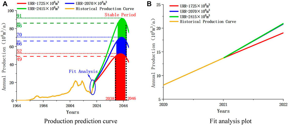
FIGURE 5. Prediction results of tight gas production based on Ward model.

In Figure 5A, the stable production period is roughly between 2038 and 2046 (between the black dotted lines), with peak production occurring in 2042 or 2043. In Figure 5B, for the prediction results under different URR, the best fit with historical production is URR= $\left(2070-2415\right)\times {10}^8{m}^3$, the higher the degree of fit, the higher the accuracy of the prediction. The final peak production result should choose the prediction value with a high degree of fit. Therefore, the predicted peak production is $\left(70-91\right){\times {10}^{8}m}^3/\mathrm{a}$, the predicted results can be used as reference values for the predictions of the Hubbert and Gauss models. Next, based on the above work, the production trend of tight gas is predicted under five different URRs, and different stages are analyzed.

3.2 Prediction and fitting analysis of tight gas production

Using the Hubbert and Gauss model, the peak production of tight gas is predicted and its variation trend is studied. The five URRs were respectively substituted into Eqs 5, 11 to establish the tight gas production-time relationship of Hubbert and Gauss model (Eqs 15, 16) and tight gas production prediction results based on the Hubbert and Gauss models (Figures 6A, 7A). Among them, Eq. 15 is the production-time relation of Hubbert model, and Eq. 16 is the production-time relation of Gauss model. The model parameters covered by these formulas are: annual peak production $Q_m$, peak production time $t_m$, peak slope $b$ and standard deviation $s$. Eq. 15 corresponds to Figures 6A, and Eq. 16 corresponds to Figures 7A.

$Q=\{\begin{array}{cc}\frac{2\times 33.02}{1+\mathit{cosh}\left[0.0957\left(t-2042\right)\right]},& \mathit{U}\mathit{R}\mathit{R}=1380\times {10}^8{m}^3\\ \frac{2\times 49.29}{1+\mathit{cosh}\left[0.1143\left(t-2042\right)\right]},& URR=1725\times {10}^8{m}^3\\ \frac{2\times 68.00}{1+\mathit{cosh}\left[0.1314\left(t-2042\right)\right]},& URR=2070\times {10}^8{m}^3\\ \frac{2\times 86.03}{1+\mathit{cosh}\left[0.1425\left(t-2042\right)\right]},& URR=2415\times {10}^8{m}^3\\ \frac{2\times 105.98}{1+\mathit{cosh}\left[0.1536\left(t-2042\right)\right]},& URR=2760\times {10}^8{m}^3\end{array},(15)$

$Q=\{\begin{array}{cc}38.01\times e^{-{\left(t-2042\right)}^2/\left(2\times {14.48}^2\right),}& URR=1380\times {10}^8{m}^3\\ 54.43\times e^{-{\left(t-2042\right)}^2/\left(2\times {12.64}^2\right),}& URR=1725\times {10}^8{m}^3\\ 71.00\times e^{-{\left(t-2042\right)}^2/\left(2\times {11.63}^2\right),}& URR=2070\times {10}^8{m}^3\\ 88.00\times e^{-{\left(t-2042\right)}^2/\left(2\times {10.95}^2\right),}& URR=2415\times {10}^8{m}^3\\ 105.0\times e^{-{\left(t-2042\right)}^2/\left(2\times {10.49}^2\right),}& URR=2760\times {10}^8{m}^3\end{array}.(16)$

FIGURE 6

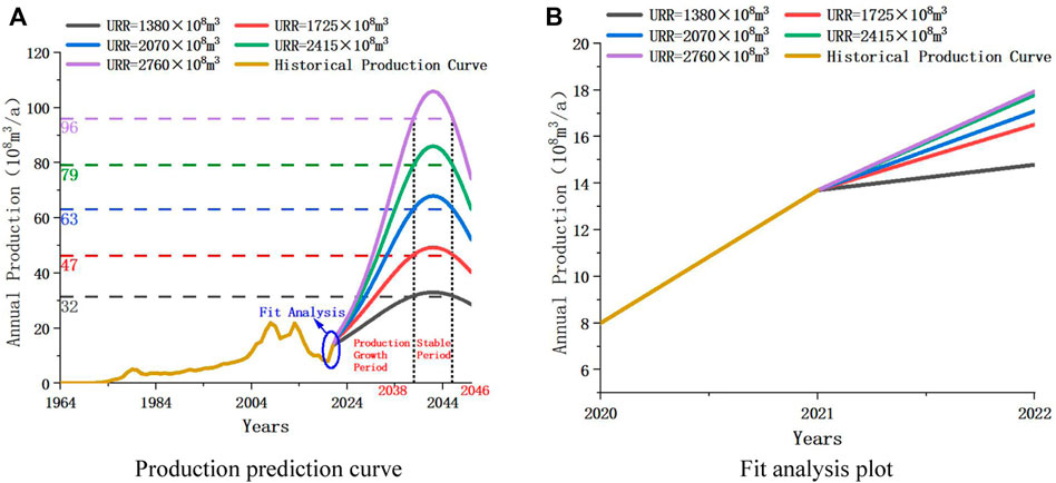
FIGURE 6. Prediction results of tight gas production based on Hubbert model.

FIGURE 7

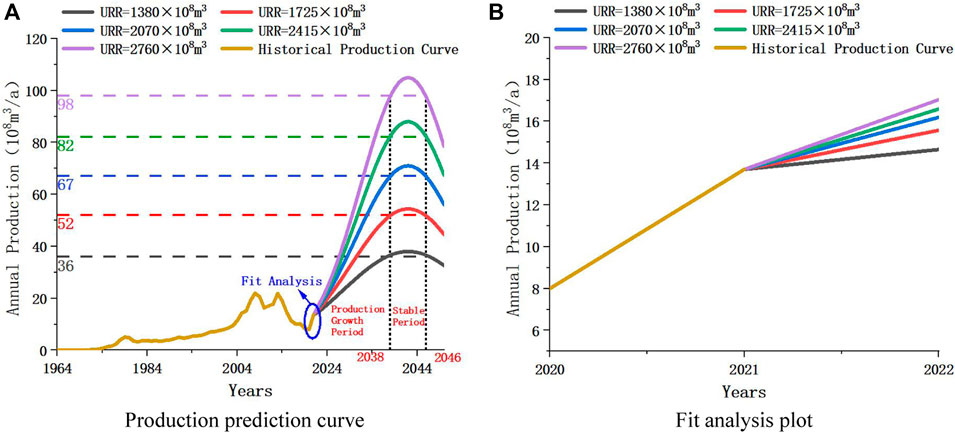
FIGURE 7. Prediction results of tight gas production based on Gauss model.

In order to deeply analyze the growth law of tight gas production with URR, it is necessary to study the relationship between the above model parameters and URR. Therefore, one hundred different URR values were uniformly sampled within the estimated range of $URR=\left(1380-2760\right)\times {10}^8{m}^3$ (Section 3.1). Substitute these URR values into Eqs 5–11 to calculate different production prediction results (Figures 6A, 7A).

It can be seen that the production prediction results in Figures 6A, 7A are highly similar. Therefore, both production prediction results can be analyzed simultaneously. The value of peak production is positively proportional to the value of URR, that is, the greater the URR is, and the greater the peak production is. The peak production always occurs in 2042, that is, $t_m\equiv 2042$, and the production growth curve is axisymmetric about $t=2042$.

According to the increase amplitude of tight gas production, the future production trend can be divided into two stages, that is, the production rising stage (2022–2038) and the production stable stage (2038–2046). In 2022–2038, production rises rapidly as the year increases. In 2038–2042, the production maintains steady growth and reaches the peak production $Q_m$ in 2042. In 2042–2046, production remains in a steady decline.

In order to compare the accuracy of production prediction results under the two different models, correlation analysis is required. This paper makes a fitting analysis diagram for the results in the early stage of prediction (Figures 6B, 7B). The fitting result represents the coincidence degree of predicted prediction and historical prediction. It can be intuitively observed from the figure that the better the fitting degree is, the closer the prediction is to the real situation, and that is, the more accurate the prediction result is.

As can be seen from the figure, for the Hubbert model, the best fit with historical production is URR= $\left(2415-2760\right)\times {10}^8{m}^3$, for the Gauss model, the best fit with historical production is URR= $2760\times {10}^8{m}^3$. And from the figure, the Hubbert model fits better than the Gauss model. After comparing the fitted graphs, this paper also calculates the correlation coefficient to determine the accuracy of the model from the perspective of data. The calculation formula is:

$r=\frac{n{\displaystyle \sum }_{i=1}^n{x}_i{y}_i-{\displaystyle \sum }_{i=1}^n{x}_i{\sum }_{i=1}^n{y}_i}{\sqrt{n{\sum }_{i=1}^n{x}_i^2-{\left({\sum }_{i=1}^n{x}_i\right)}^2}\sqrt{n{\sum }_{i=1}^n{y}_i^2-{\left({\sum }_{i=1}^n{y}_i\right)}^2}}.(17)$

In the formula, r is the correlation coefficient, n is the number of data points, and $x_i$ and $y_i$ are the coordinate values of each point.

The correlation coefficient method can directly reflect the correlation degree between two groups of variables, which can be used as one of the judgment criteria for the accuracy of prediction results. The correlation coefficients of the production prediction results of the two models under different URRs are shown in Table 2. It can be seen from the table that the correlation coefficients of the two models are very close to 1, and the corresponding production prediction results are very accurate. However, the correlation coefficients of the predicted results of the Hubbert model under each URR are higher than those of the Gauss model. The higher the correlation coefficient is, the more accurate and representative the prediction result is. Therefore, the prediction data of the Hubbert model is selected as the prediction result of tight gas production. In addition, since the Hubbert model has the highest fitting degree under URR= $\left(2415-2760\right)\times {10}^8{m}^3$, the final peak range should also correspond to it.

TABLE 2

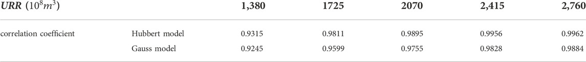
TABLE 2. Correlation coefficient of production prediction results.

3.3 Overview

The low degree of exploration and development of tight gas leads to many unknown factors. Therefore, the ultimate recoverable reserves URR is introduced into the study of production change trend as a main factor. The final range of peak production was calculated by defining the value range of URR, and Hubbert and Gauss model were established to realize the calculation. The accuracy of the results was judged by comparing the results of the correlation coefficients and referring to the degree of fitting of the predictions. Establishing a prediction model for the growth trend of tight gas production under different proven rates can provide a theoretical basis for tight gas exploration and development planning. The production results predicted by the Hubbert model are shown in Table 3.

TABLE 3

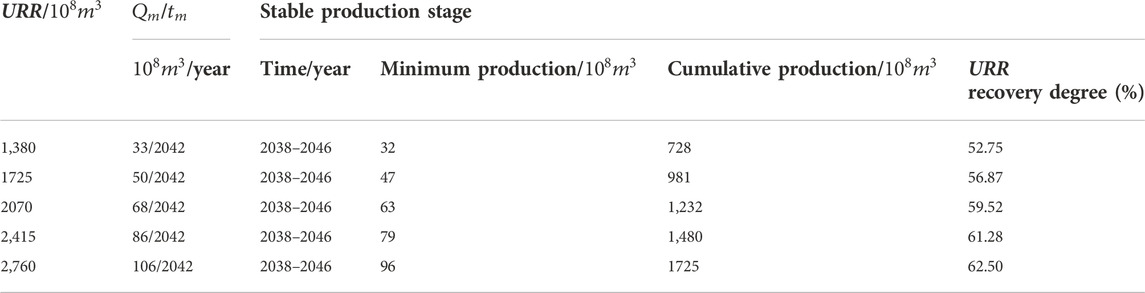
TABLE 3. Prediction results of tight gas production under different URR conditions.

Preliminary prediction results show that tight gas production in the Sichuan Basin will continue to maintain a rapid growth trend in the next 20 years. According to the fitting degree and correlation analysis between the predicted results and historical production, the production of tight gas will reach the peak range of $\left(86-106\right){\times {10}^{8}m}^3/\mathrm{a}$ in 2042. At the end of the stable production period, the URR recovery was about 60%.

4 Tight gas production risk quantification

4.1 Realization probability analysis combined with Monte Carlo principle

As described in Section 3.2, the production growth process for future time periods is divided into two stages. That is, the production rising stage (2022–2038) and the production stable stage (2038–2046). Therefore, it is necessary to calculate and analyze the production realization probability for different production growth stages.

In order to clearly describe the influence of URR on production prediction results, the variation trend of peak production and model parameters under different URRs was first analyzed and studied. As shown in Figure 8, with the increase of URR, the peak production $Q_m$ and the model parameter b both keep increasing trend on the whole. However, in a certain area where the URR does not change significantly, $Q_m$ and b show a negative correlation trend, that is, when $Q_m$ increases, b decreases. This law corresponds to Eq. 4. Then zoom in on the prediction results of the two production growth stages in Figures 6A, and change the abscissa of these figures from year to URR. The URR-production prediction results of each stage and year can be obtained (Figure 9).

FIGURE 8

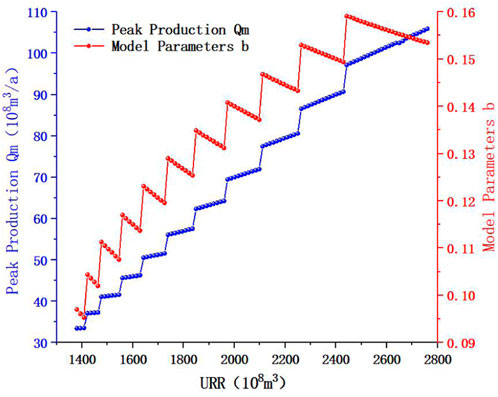
FIGURE 8. Peak production versus model parameters.

FIGURE 9

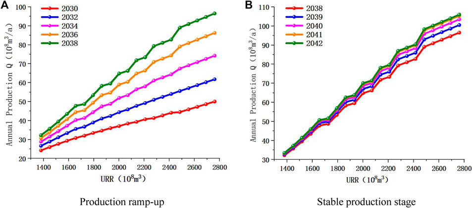
FIGURE 9. URR-production prediction result graph.

It can be seen from Figure 9 that the change trend of annual production with URR is consistent with the change trend of peak production in Figure 8, regardless of whether it is a rising stage or a stable stage. This law corresponds to Eq. 4. Therefore, it can be considered that with the increase of URR, the annual production shows a step-like growth trend. At the same time, with the increase of URR, the interval between the production curves of different years is larger, which shows that the increase of URR also leads to the increase of annual production growth rate. This also explains that in Figure 6, the larger the URR, the greater the slope of the production prediction curve, and the greater the production increase.

To calculate the different production realization probabilities for each year of the two production growth stages, the Monte Carlo method described in Section 2.2.1 was applied. Take 2030 as an example to introduce the probability analysis process of tight gas production. Taking the Hubbert production calculation equation of Eq. 5 as the mathematical model of probability simulation, URR is the main independent variable affecting production. Since the value of URR is obtained by uniform sampling (Section 3.2). Therefore, uniformly distributed URR values are directly drawn at random multiple times. Set the number of URR extractions to 10,000 times. For each URR value extracted, calculate the corresponding $Q_m$ and $t_m$ values, and substitute them into Eq. 5 together with t = 2030 to obtain the production Q in 2030.

The production of a certain year is repeatedly calculated by cycle. After 10,000 cycles, the distribution probability of the target production can be achieved is obtained, and then the cumulative probability is calculated according to the distribution probability. That is, the probability at the minimum point of annual production is 1, the probability at the next point of production is equal to 1 minus the sum of the distribution probabilities of all previous production, and so on up to the maximum point of annual production. The distribution probability is the average probability of each production value point under the normal distribution, the sum is 1, and the cumulative probability is the realization probability of annual production.

Since the URR is uniformly distributed, the accuracy of the production probability statistics can be guaranteed. Figure 10 shows the production realization probability results for representative years in the 2 phases. As can be seen from Figure 10, for the distribution probability, its changing trend is similar to the normal distribution. That is, in the same year, the closer the production is to the extreme value, the lower the probability, and the closer to the middle value, the higher the probability. For cumulative probability, the lower the production value, the higher the realization probability.

FIGURE 10

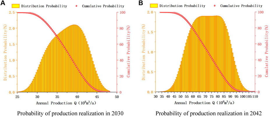
FIGURE 10. Production-realization probability plot in different years.

Figure 11A is a graph of the production realization probability of each year during the stable production period. It can be seen from the figure that with the increase of the annual production prediction value, the realization probability gradually decreases. At the same time, the production corresponding to the realization probability of 10%–20% is the ideal production, and the ideal production in the stable production period under the prediction model is stable between $\left(80-90\right){\times {10}^{8}m}^3/\mathrm{a}$. Figure 11B shows the prediction of annual production under different probabilities (realization probability 10%–90%), where P90 indicates that the probability is 90%. It can be seen from the figure that the change trend of annual production under different probabilities is basically the same, and the production values of adjacent probabilities are also roughly the same. This indicates that the production change trend under the prediction model is relatively stable, and the prediction results are more accurate.

FIGURE 11

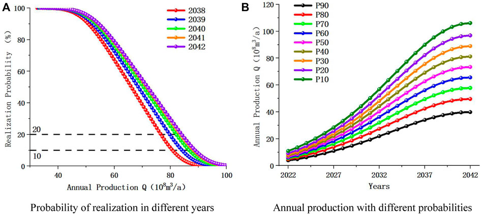
FIGURE 11. Production - realization probability trend chart.

Table 4 represents the production values that can be achieved in several major years under different probability scenarios. The probability is the cumulative probability, so cumulative probability is also realization probability. In 2042, $\mathrm{P}20=96.89{\times {10}^{8}m}^3/\mathrm{a}$ means that the probability of production reaching $96.89{\times {10}^{8}m}^3/\mathrm{a}$ is 20%. In this paper, the production of tight gas is calculated in the probability interval of 0%–100%, and the risk quantification of production in different probability intervals. Among them, the production corresponding to P80 is the guaranteed production, the production corresponding to P50 is the average production, and the production corresponding to P20 is the ideal production. The probability values calculated by Monte Carlo method represent the possibility of achieving tight gas production in different periods. This feasibility study has an important guiding role for the planning of tight gas production in the future.

TABLE 4

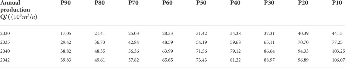
TABLE 4. Calculation results of production realization probability in different stages and years.

4.2 Production risk level evaluation based on matrix analysis

In order to conduct risk quantification research on tight gas production, the risk matrix (Figure 3) in Section 2.2.2 needs to be introduced to evaluate the production risk level. According to the probability calculation method in Section 2.2, the production distribution probability and realization probability curve of each year in the two stages were obtained respectively. According to the distribution probability curve, the mean value $\mu$ and the standard deviation $s$ of the annual production are obtained, so as to obtain the dispersion degree $C$ of the annual production according to Eq. 14.

In the rising stage of production, $5\%<C\le 10\%$. At this time, the annual production corresponding to $P>50\%$ is a risk level II, the annual production corresponding to $20\%\le P<50\%$ is a risk level III, and the annual production corresponding to $P<20\%$ is a risk level IV.

In the stable production stage, $10\%<C\le 25\%$. At this time, the annual production corresponding to $P>50\%$ is a risk level III, and the annual production corresponding to $P\le 50\%$ is a risk level IV.

Since the dispersion degree is different in different stages, the risk level of production target in different stages and years can be obtained by combining the dispersion degree and realization probability. (Figure 12) (Guo et al., 2022).

FIGURE 12

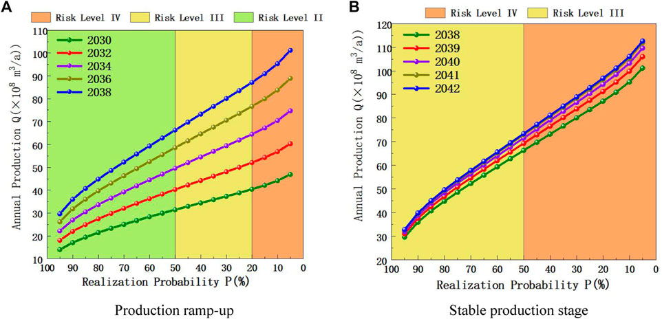
FIGURE 12. Production risk level assessment.

It can be known from Figure 11 that the higher the target production is, the lower the corresponding realization probability value is, and the production -probability curve is also in the region with higher risk level. According to the production risk quantification results of different stages in Figure 12, the realization probability and risk level of different productions in each year can be directly obtained. Production risk level indicates how easy it is to achieve the production target, therefore, combined with the realization probability calculation and risk level evaluation, the risk quantification of production can be well studied, and the realization probability of tight gas target production can be calculated, which provides data support for feasibility analysis.

4.3 Overview

The quantitative research on tight gas production risk is based on the production prediction results. According to the uniformly distributed proved rate, URR of different degrees is calculated, and the probability of achieving the target production in different stages is studied to obtain the possibility of achieving the tight gas production in different years. Combined with the realization probability and the degree of dispersion, the risk grade analysis was used to evaluate the annual production in different stages of production growth. The target risk of tight gas production is comprehensively analyzed.

At present, the exploitation of tight gas in the Sichuan Basin is still in its early stage, and the production prediction and risk quantification of tight gas are also in the shallow stage. In this paper, URR was introduced as the influencing factor of production change trend by using the proved rate as the medium, without more comprehensive quantitative research considering other factors. Risk assessment is based on the results of production prediction and studies the degree of difficulty to achieve the target production. Therefore, the production prediction and risk assessment of tight gas need to carry out more research work, so as to provide a better reliable basis for tight gas production planning.

5 Conclusion

1) According to the uniformly distributed proved rate, URR was introduced as the main factor, and Hubbert and Gauss models were respectively used to predict the variation trend of tight gas production. According to the curve fitting results and correlation size, the accuracy of Hubbert model is higher, and the predicted results of this model are finally adopted. According to the amplitude of production change, the process of production increase is divided into two stages, namely, production increase stage and production stability stage. The production prediction results show that the tight gas production will reach the peak range of $\left(86-106\right){\times {10}^{8}m}^3/\mathrm{a}$ in 2042. And the production will be stable from 2038 to 3046, and the URR recovery degree will be about 60% at the end of the stable production period.

2) Based on the results of tight gas production prediction and risk assessment combined with the realization probability and dispersion degree, the possibility of achieving different target production can be intuitively obtained, and finally provides a basis for the planning of tight gas production. According to the Monte Carlo method, the production change curve is analyzed, and the production realization probability of different years in each stage is calculated, and then the risk assessment of tight gas production is carried out based on the dispersion degree. Finally, the establishment of the target risk quantification system for tight gas production in the Sichuan Basin was promoted.

3) Sun et al. (2021), Wang et al. (2018), JamesWard et al. (2012) and others all predicted natural gas production from the perspective of single prediction. In this paper, according to the actual situation of Sichuan Basin and the lack of historical tight gas data, Word model was first used to predict the peak production and the range of peak time, and then Hubbert model and Gauss model were combined to predict. Combining with the degree of fitting and the calculation of correlation coefficient of prediction results, a more accurate model was determined. Based on the Monte Carlo method and the risk matrix principle, the realization probability of future production was predicted, and the risk assessment of tight gas production was carried out by combining the realization probability and dispersion degree. In this paper, a new idea was adopted on the combination and progression of the methods, which can provide a reference for the prediction of gas reservoirs with few historical data.

Data availability statement

The raw data supporting the conclusion of this article will be made available by the authors, without undue reservation.

Author contributions

HL and GY provide technical support, theoretical basis and on-site guidance; YF provides data basis and algorithm process; YC processes data and writes papers; and DZ reviews and modifies them.

Funding

This study was financially supported by the Scientific Research Foundation of State Key Laboratory of Coal Mine Disaster Dynamics and Control (2011DA105287-zd201804).

Conflict of interest

HL and YF were employed by Exploration and Development Research Institute of PetroChina Southwest Oil and Gas Field Company. GY was employed by PetroChina Southwest Oil and Gas Field Company Planning Department.

The remaining authors declare that the research was conducted in the absence of any commercial or financial relationships that could be construed as a potential conflict of interest.

Publisher’s note

All claims expressed in this article are solely those of the authors and do not necessarily represent those of their affiliated organizations, or those of the publisher, the editors and the reviewers. Any product that may be evaluated in this article, or claim that may be made by its manufacturer, is not guaranteed or endorsed by the publisher.

References

Chengzao, J., Yongfeng, Z., and Xia, Z. (2014). Prospects of and challenges to natural gas industry development in China. Nat. Gas. Ind. B 1, 1–13. doi:10.1016/j.ngib.2014.10.001

CrossRef Full Text | Google Scholar

Chong, L., Wu., W.Z., Xie., W., Zhang, T., and Zhang, J. (2021). Forecasting natural gas consumption of China by using a novel fractional grey model with time power term. Energy Rep. 7, 788–797. doi:10.1016/j.egyr.2021.01.082

CrossRef Full Text | Google Scholar

Dai, Jinxing., Ni, Yunyan., Liu, Quanyou., Wu, X., Gong, D., Hong, F., et al. (2021). Sichuan super gas basin in southwest China. Petroleum Explor. Dev. 48 (2), 1251–1259. doi:10.1016/s1876-3804(21)60284-7

CrossRef Full Text | Google Scholar

Flouri., M., Karakosta., C., Kladouchou., C., and Psarras, J. (2015). How does a natural gas supply interruption affect the EU gas security? A Monte Carlo simulation. Renew. Sustain. Energy Rev. 44, 785–796. doi:10.1016/j.rser.2014.12.029

CrossRef Full Text | Google Scholar

Gabriel, M. P., Bruno, F., Josiane, S. C., Flávia, M., Fabio, O., João, J. R., et al. (2021). Evaluation of characteristic diameter on barite settling in drilling fluids by Monte Carlo method. J. Petroleum Sci. Eng.

Google Scholar

Guo, Y., Chen, Y., Li, H., Liu, L., Wang, C., Chen, Y., et al. (2022). Studies on natural gas production prediction and risk quantification of Sinian gas reservoir in Sichuan Basin. J. Pet. Explor. Prod. Technol. 12 (4), 1109–1120. doi:10.1007/s13202-021-01368-y

CrossRef Full Text | Google Scholar

Guo, Y., Fang, Y., Li, H., Wang, C., and Zhang, D. (2021). Establishment and application of prediction model of natural gas reserve and production in Sichuan Basin. J. Pet. Explor. Prod. Technol. 11 (6), 2679–2689. doi:10.1007/s13202-021-01189-z

CrossRef Full Text | Google Scholar

Gutierrez, J. P., Benitez, L. A., Ruiz, E. A., and Erdmann, E. (2016). A sensitivity analysis and a comparison of two simulators performance for the process of natural gas sweetening. J. Nat. Gas Sci. Eng. 31 (11), 800–807. doi:10.1016/j.jngse.2016.04.015

CrossRef Full Text | Google Scholar

Höök, M., Li, J., Johansson, K., and Snowden, S. (2012). Growth rates of global energy systems and future outlooks. Nat. Resour. Res. 21 (1), 23–41. doi:10.1007/s11053-011-9162-0

CrossRef Full Text | Google Scholar

Hu, Yong., Wenxiang, He., and Guo, Bincheng. (2020). Combining sedimentary forward modeling with sequential Gauss simulation for fine prediction of tight sandstone reservoir. Mar. Petroleum Geol. 112, 104044. doi:10.1016/j.marpetgeo.2019.104044

CrossRef Full Text | Google Scholar

Huang., Y., Ai, W., Xiao., K., Lin, T., and Jin, W. (2022). Types and Genesis of sweet spots in the tight sandstone gas reservoirs:Insights from the Xujiahe Formation, northern Sichuan Basin, China. Energy Geosci. 3, 270–281. doi:10.1016/j.engeos.2022.03.007

CrossRef Full Text | Google Scholar

JamesWard., D., Mohr., Steve H., Myers., Baden R., and Nel, W. P. (2012). High estimates of supply constrained emissions scenarios for long-term climate risk assessment. Energy Policy 51, 598–604. doi:10.1016/j.enpol.2012.09.003

CrossRef Full Text | Google Scholar

Jia, Ailin (2018). Progress and prospects of natural gas development technologies in China. Nat. Gas. Ind. B 5, 547–557. doi:10.1016/j.ngib.2018.11.002

CrossRef Full Text | Google Scholar

Krupenev., Dmitry, Denis, Boyarkin., and Iakubovskii., Dmitrii (2020). Improvement in the computational efficiency of a technique for assessing the reliability of electric power systems based on the Monte Carlo method. Reliab. Eng. Syst. Saf. 204, 107171. doi:10.1016/j.ress.2020.107171

CrossRef Full Text | Google Scholar

Lao., Tongfei, and Sun., Yanrui (2022). Predicting the production and consumption of natural gas in China by using a new grey forecasting method. Math. Comput. Simul. 202, 295–315. doi:10.1016/j.matcom.2022.05.023

CrossRef Full Text | Google Scholar

Lin, Jiang., Wen, Zhao., Yang, Fan., Hong, F., Gong, Y., and Hao, J. (2021). Effects of micro-fracture and micro-coal line on tight gas accumulation, Triassic Xujiahe Formation, Sichuan Basin, China. Energy Rep. 7, 7913–7924. doi:10.1016/j.egyr.2021.08.185

CrossRef Full Text | Google Scholar

Luz-Sant’Ana, P., Roman-Roman, I., Torres-Ruiz., F, and Torres Ruiz, F. (2017). Modeling oil production and its peak by means of a stochastic diffusion process based on the Hubbert curve. Energy 133, 455–470. doi:10.1016/j.energy.2017.05.125

CrossRef Full Text | Google Scholar

Mohr, S. H., and Evans, G. M. (2011). Long term forecasting of natural gas production. Energy Policy 39, 5550–5560. doi:10.1016/j.enpol.2011.04.066

CrossRef Full Text | Google Scholar

Ravnik, J., Jovanovac, J., Trupej, A., Vistica, N., and Hribersek, M. (2021). A sigmoid regression and artificial neural network models for day-ahead natural gas usage forecasting. Clean. Responsible Consum. 3, 100040. doi:10.1016/j.clrc.2021.100040

CrossRef Full Text | Google Scholar

Shih-Chi, Lo., Ma, Hwong-wen, and Lo, Shang-Lien (2005). Quantifying and reducing uncertainty in life cycle assessment using the Bayesian Monte Carlo method. Sci. Total Environ. 340, 23–33. doi:10.1016/j.scitotenv.2004.08.020

PubMed Abstract | CrossRef Full Text | Google Scholar

Sun, Y., Rahmani, A., Saeed, T., Zarringhalam, M., Ibrahim, M., and Toghraie, D. (2021). Simulation of deformation and decomposition of droplets exposed to electro-hydrodynamic flow in a porous media by lattice Boltzmann method. Alexandria Eng. J.

Google Scholar

Tilton, J. E. (2018). The Hubbert peak model and assessing the threat of mineral depletion. Resour. Conservation Recycl. 13 (9), 280–286. doi:10.1016/j.resconrec.2018.08.026

CrossRef Full Text | Google Scholar

Tong, Xiaoguang., Zhang, Guangya., Wang, Zhaoming., Wen, Z., Tian, Z., Wang, H., et al. (2018). Distribution and potential of global oil and gas resources. Petroleum Explor. Dev. 45, 779–789. doi:10.1016/s1876-3804(18)30081-8

CrossRef Full Text | Google Scholar

Wang, H., Ma, F., Tong, X., Liu, Z., Zhang, X., Wu, Z., et al. (2016a). Assessment of global unconventional oil and gas resources. Petroleum Explor. Dev. 43, 925–940. doi:10.1016/s1876-3804(16)30111-2

CrossRef Full Text | Google Scholar

Wang, J., Jiang, H., Zhou, Q., Wu, J., and Qin, S. (2016b). China's natural gas production and consumption analysis based on the multicycle Hubbert model and rolling Grey model. Renew. Sustain. Energy Rev. 53 (11), 1149–1167. doi:10.1016/j.rser.2015.09.067

CrossRef Full Text | Google Scholar

Wang, Q., Li, S., Li, R., and Ma, M. (2018). Forecasting U.S. shale gas monthly production using a hybrid ARIMA and metabolic nonlinear grey model. Energy 16 (10), 378–387. doi:10.1016/j.energy.2018.07.047

CrossRef Full Text | Google Scholar

Wang., J., Lian., S., Lei., B., Li, B., and Lei, S. (2022). Co-training neural network-based infrared sensor array for natural gas monitoring. Sensors Actuators A Phys. 335, 113392. doi:10.1016/j.sna.2022.113392

CrossRef Full Text | Google Scholar

Ward, P. G., Thaw Tar, T. Z., Wang., M., Dauwels, J., and Ukil, A. (2018). Leak detection in low-pressure gas distribution networks by probabilistic methods. J. Nat. Gas Sci. Eng. 58, 69–79. doi:10.1016/j.jngse.2018.07.012

CrossRef Full Text | Google Scholar

Wu, X., Chen, Y., Wang, Y., Zeng, H., Jiang, X., and Hu, Y. (2021b). Geochemical characteristics of natural gas in tight sandstone of the Chengdu large gas field, Western Sichuan Depression, Sichuan Basin, China. J. Nat. Gas Geoscience 6, 279–287. doi:10.1016/j.jnggs.2021.09.003

CrossRef Full Text | Google Scholar

Yiping, W., Buqing, S., Jianjun, W., Qing, W., Haowu, L., Zhanxiang, L., et al. (2021a). An improved multi-view collaborative fuzzy C-means clustering algorithm and its application in overseas oil and gas exploration. J. Petroleum Sci. Eng. 197, 108093. doi:10.1016/j.petrol.2020.108093

CrossRef Full Text | Google Scholar

Zeng., B., Xin, M., and Meng, Z. (2020). A new-structure grey Verhulst model for China’s tight gas production forecasting. Appl. Soft Comput. 96, 106600. doi:10.1016/j.asoc.2020.106600

CrossRef Full Text | Google Scholar

Zhang, K., and Zhao, Y. (2021). Modeling dynamic dependence between crude oil and natural gas return rates: A time-varying geometric copula approach. J. Comput. Appl. Math. 386 (4), 113243. doi:10.1016/j.cam.2020.113243

CrossRef Full Text | Google Scholar

Zheng, C., Wu, W., Xie, W., and Li, Q. (2020). A MFO-based conformable fractional nonhomogeneous grey Bernoulli model for natural gas production and consumption forecasting. Appl. Soft Comput. 11 (6), 106891. doi:10.1016/j.asoc.2020.106891

CrossRef Full Text | Google Scholar

Zheng, Y., Han, Xu., Zeng, Ji., Zhou, C., Zhou, L., and Chen, W. (2021). Practice of high-intensity volume fracturing in the Shaximiao Formation tight sandstone gas reservoirs of the Qiulin Block, central Sichuan Basin. Nat. Gas. Ind. B 8, 367–375. doi:10.1016/j.ngib.2021.07.007

CrossRef Full Text | Google Scholar