Comparison of the Dynamic and Static Corner Frequencies in Ground Motion Simulation: Cases Study of Jiuzhaigou Earthquake and Northridge Earthquake

By using the stochastic finite-fault method based on static corner frequency (Model 1) and dynamic corner frequency (Model 2), we calculate the far-field received energy (FRE) and acceleration response spectra (SA) and then compare it with the observed SA. The results show that FRE obtained by the two models depends on the subfault size regardless of high-frequency scaling factor (HSF). Considering the HSF, the results obtained by Model 1 and Model 2 are found to be consistent. Then, similar conclusion was obtained from the Northridge earthquake. Finally, we analyzed the reasons and proposed the areas that need to be improved.

Introduction

The abundance of earthquake disaster investigation results indicated that the main factor that causes the destruction and collapse of a building or structure is ground motion. In addition, ground motion also induces many natural disasters, such as soil liquefaction, mountain collapse, and landslides and debris flows. Recordings of the ground motion can play an essential role in studying the basic data for earthquake-resistant design. However, for countries and regions that lack strong ground-motion data, it is necessary to synthesize acceleration time histories based on engineering experience and research results in areas with rich strong ground-motion data. Currently, three main methods, namely, the deterministic method, stochastic method, and hybrid broadband simulation method, are used for simulating and predicting ground motion. The deterministic method is mainly based on the displacement representation theorem of Aki and Richards (1980), which expresses the ground motion as a convolution of the source time function and Green’s function in the frequency domain. This method is primarily used for low-frequency simulations. The stochastic method was proposed and advanced by Boore based on the random vibration theory of band-limited windowed Gaussian noise (Boore, 1983; Boore, 2003), and it is mainly used for high-frequency ground motion simulations. The hybrid simulation method employs the first two methods for simulating the low-frequency and high-frequency bands separately and subsequently performs filtering and superposition to obtain the effect of wideband simulation (Graves and Pitarka, 2004; Motazedian and Moinfar, 2006; Frankel, 2009; Graves and Pitarka, 2010). However, since the stochastic point-source method can only be applied to small earthquakes, Beresnev and Atkinson proposed a stochastic finite-fault approach (FINSIM) to overcome this limitation (Beresnev and Atkinson, 1998a; Beresnev and Atkinson, 1998b). Basically, the main fault is divided into multiple subfaults in this method, and each subfault is considered a stochastic point-source (Hartzell, 1978). A rupture shows rapid spreading from the hypocenter. Our scheme employs the stochastic point-source method for calculating the acceleration time series of each subfault (Boore, 1983; Boore, 2003). Then, to obtain the ground-motion acceleration from the main fault, the ground motions of subfaults are summed with a proper time delay in the time domain. However, the far-field received energy obtained based on the stochastic finite-fault approach strongly depends on the subfault size (Beresnev and Atkinson, 1998a; Beresnev and Atkinson, 1998b). To guarantee that the far-field received energy is equivalent to the stochastic point-source method, the subfault size must be strictly controlled. Motazedian and Atkinson (2005) reported a dynamic corner frequency and introduced a high-frequency scaling factor. As a result, the far-field received energy is not influenced by the size of the subfault. Some scholars have compared the stochastic point-source method (SMSIM) and the stochastic finite-fault method (EXSIM) and further improved the stochastic finite-fault method (Boore, 2009; Toni, 2017). This process included 1) changing the duration of motions from each subfault to the inverse of the subfault corner frequency, 2) calculating the high-frequency scaling factor based on the integral of the squared Fourier acceleration spectrum rather than the Fourier velocity spectrum, and 3) adding a filter function and a near-fault velocity pulse by considering the directivity effect (Mavroeidis and Papageorgiou, 2003). Consequently, the stochastic point-source and stochastic finite-fault can produce consistent motions based on a remote earthquake with a low moment magnitude, thus making ground-motion simulations no longer dependent on the subfault number.

According to Boore (2003), the stochastic simulation method has been widely applied in practical engineering due to its simplicity and low number of input parameters. It has been proven to be the most effective technique for simulating ground motions, especially at a frequency of greater than 1 Hz (Chopra et al., 2012; RaghuKanth and Kavitha, 2013; Zafarani et al., 2015; Dang and Liu, 2020; Tanırcan and Yelkenci-Necmioğlu, 2020; Sutar et al., 2020; Sharma et al., 2021; Dang et al., 2021). Boore improved and modified the stochastic finite-fault approach, and thus, it was extensively used and followed by numerous scholars in simulating high-frequency ground motions (Boore and Thompson, 2015).

Based on the above discussion, the static corner frequency and the dynamic corner frequency are exploited to evaluate the far-field received energy of an observation point with an epicentral distance of 333 km. The original slip distribution was provided by Zheng et al. (2017). In our scheme, the main fault is categorized into different subfault lengths, such as 1, 2, 3, and 6 km, and the corresponding amount of slip distribution is given to each subfault according to the original slip distribution (Zheng et al., 2017). In addition, by using the same method, the acceleration time series of the 1994 Northridge earthquake in the United States can also be obtained.

Simulation Method

Stochastic Point-Source Model (SMSIM)

The stochastic point-source method was proposed by Boore. (1983), Boore (2003). Initially, this method assumes that the fault size is much smaller than the distance from the source to the observation point. Consequently, the source can be considered as a small point source. According to the assumption, the high-frequency ground motions can be observed as band-limited windowed Gaussian noise in the elastic half-space. During this point of time, in the frequency domain, the ground-motion Fourier amplitude spectrum of an observation point can be expressed as follows:

$A_{ij}\left(M_0,f,R\right)=E\left(M_0,f\right)P\left(R,f\right)G\left(f\right)I\left(f\right)(1)$

where A_ij (M₀, f, R) denotes the Fourier amplitude spectrum of the ground motion, which can be acceleration, velocity, or displacement. E(M₀, f) denotes the source term; P(R, f) stands for the path term; G(f) is the site term; I(f) is the instrument or type of the site ground-motion response (see Boore, 1983; Boore, 2003 for the particular meaning of these terms); M₀ represents the seismic moment (dyne-cm); R stands for the shortest distance from the fault to the site (km); and f refers to the frequency (Hz). The filter I(f) controls the type of ground motion that originates from the ground-motion simulation. When the ground motion is desired, I(f) = (2πfi)ⁿ, in which i is the imaginary unit (i = (−1)^0.5) and n = 0, 1, or 2 for ground displacement, velocity, or acceleration, separately.

Stochastic Finite-Fault Model Based on Static Corner Frequency (Model 1)

To overcome the inability to express directivity effects in stochastic point source simulating ground motion and not applicable to small earthquakes, Beresnev and Atkinson. (1998a), Beresnev and Atkinson. (1998b) developed FINSIM. Although there has been an empirical calibration of the subfault dimension in FINSIM, in this study, we added a high-frequency scaling factor to the FINSIM method and use corner frequency (Eq. 2) instead of the original corner frequency, which is defined by Beresnev and Atkinson (1998a) in the form of f_c = yz/π(β/△l), in which y, z and π are constant, β is the shear wave velocity in km/s, and △l is the subfault size. We divided the entire fault into several subfaults, and assumed that the corner frequency of the ijth subfault is equal to the static corner frequency, which can be expressed as follows:

$f_0=4.9\times {10}^6\beta \left(\mathrm{\Delta }\sigma /M_0\right)(2)$

Generally, the source spectrum of the ijth subfault can be expressed as follows:

$S_{ij}\left(f\right)=\frac{C{M}_{0ij}{H}_{ij}}{1+{\left(f/f_0\right)}^2}(3)$

where C is a constant (Boore, 2003); H_ij denotes the scaling factor at high frequency, which conserves the subfault spectral level at high frequency; and f₀ and M_0ij denote the corner frequency and seismic moment of the ijth subfault, respectively.

In the original FINSIM method, to ensure the seismic moment conservation of the entire fault, some faults often need to be triggered many times, which is difficult to give a reasonable explanation in physics. However, in our Model 1, each subfault breaks up to one time, and the seismic moment of each subfault is calculated based on its area to the total fault area ratio. Specifically, the seismic moment for every subfault can be determined according to the following formula in the case of different subfaults (Motazedian and Atkinson, 2005):

$M_{0ij}=M_0\frac{D_{ij}}{{\displaystyle \sum _{k=1}^{nl}{\displaystyle \sum _{l=1}^{nw}{D}_{ij}}}}(4)$

where D_ij denotes the ijth subfault slip; nw and nl represent subfault number along the dip and strike directions, respectively (nl × nw = N); and M₀ represents the seismic moment of the entire fault.

The high-frequency scaling factor defined based on the square of the acceleration spectrum is used to obtain the far-field received energy conservation, which can be calculated by the following formula (Boore, 2009):

$H_{ij}=\sqrt{\frac{N{\displaystyle \sum \{f^2/{\left[1+{\left(f/f_0\right)}^2\right]\}}^2}}{{\displaystyle \sum \{f^2/{\left[1+{\left(f/f_{0ij}\right)}^2\right]\}}^2}}}(5)$

where f₀ stands for the static corner frequency defined by Eq. 2. N is the numbers of subfaults on the whole fault. In Model 1, because the corner frequency of the ijth subfault is equal to the static corner frequency, then H_ij is equal to N^1/2, that is, the Fourier acceleration spectra from Model 1 should be multiplied by N^1/2 (Boore, 2009).

Stochastic Finite-Fault Model Based on Dynamic Corner Frequency (Model 2)

Taking into consideration the limitations of the static corner frequency, the dynamic corner frequency was developed by Motazedian and Atkinson (2005), which determines the source spectrum of the ijth subfault as follows:

$S_{ij}\left(f\right)=\frac{C{M}_{0ij}{H}_{ij}}{1+{\left(f/f_{0ij}\right)}^2}(6)$

where M_0ij denotes the seismic moment of the ijth subfault, which can be obtained by Eq. 4.

The dynamic corner frequency of every subfault is determined according to the following formula:

$f_{0ij}=4.9\times {10}^6\beta {\left(\frac{\mathrm{\Delta }\mathrm{\sigma }}{M_{0ave}}\right)}^{1/3}\times N{\left(t\right)}_{ij}^{-1/3}(7)$

where M_0ave denotes the mean seismic moment of subfaults (M_0ave = M₀/N) and N(t)_ij represents the subfault cumulative number rupturing at time t. According to the dynamic corner frequency formula, the subfault corner frequency is represented by the inverse proportion to the 1/3 power of the active subfault number and the mean seismic moment. The subfault corner frequency is observed to be the greatest where the rupture starting point is located. With the extension of rupture, the latter subfault that ruptures always shows reduced corner frequency compared to the former subfault. Due to the scaling factor at high frequency and the dynamic corner frequency, the simulated acceleration Fourier spectrum no longer depends on the subfault size. Nonetheless, the corner frequency of every subfault can be calculated based on its rupture order rather than the subfault slip. Therefore, the dynamic corner frequency cannot represent the seismic wave radiation frequency heterogeneity as a result of slip distribution.

As the amplitude spectrum of the subfaults is approximately proportional to the square of the corner frequency at high frequencies, except for the fracture initiation point and several subfaults in the vicinity of the starting point, the corner frequency of the other subfaults is found to be small, which inevitably causes the underestimation of the amplitude spectrum of the ground motion at high frequencies. To compensate for this underestimation caused by the dynamic corner frequency, Motazedian and Atkinson (2005) proposed a high-frequency scaling factor, H_ij, to ensure the conservation of the far-field received energy considering the fact that the far-field received energy is in proportion to the square of the velocity spectrum. In Model 2, the high-frequency scaling factor also defined by Eq. 5, in which the corner frequency of the ijth subfault can be obtained from Eq. 7, and f₀ denotes the corner frequency of the main fault, which can be calculated by Eq. 2.

To make the results of the stochastic finite-fault method consistent with those of the stochastic point-source method for small and large earthquakes at close and far distances, Boore (2009) modified the filter function to compensate for the underestimation at low frequencies caused by incoherent summation.

Finally, considering the combined effect of the filter function and the high-frequency scaling factor, the Fourier amplitude spectrum of certain observation point has the tendency to be N^−1/2 times larger at low frequencies. Both the EXSIM and SMSIM simulations are found to be in close conformity with one another, and the EXSIM results do not depend on the number of subfaults. Meanwhile, the underestimation caused by incoherent summation at low frequencies is also eliminated. Additionally, the Fourier acceleration spectrum obtained by EXSIM exhibits similar results to that of SMSIM for a small earthquake at a large distance.

In the near-fault ground-motion simulation, the main fault is usually divided into rectangular subfaults of equal size. Each subfault can be approximately described as a small point source. In addition, the whole fracture process can be expressed as a series of subfaults superimposed in a certain order. According to Beresnev and Atkinson (1998a), for every subfault, rupture propagates to the center, and a subfault triggers when the rupture propagates to the subfault center. The SMSIM was used to calculate accelerations a_ij(t) (Boore, 1983; Boore, 2003). The accelerations generated by all subfaults are summarized in the time domain with appropriate delay:

$a\left(t\right)={\displaystyle \sum _{i=1}^{nl}{\displaystyle \sum _{j=1}^{nw}{a}_{ij}\left(t+\mathrm{\Delta }{t}_{ij}\right)}}(8)$

where △t_ij includes the time delay from the starting point to the subfault and the path delay from the subfault to the observation point.

Database and Model Parameters

Jiuzhaigou Earthquake

In the case of the Jiuzhaigou earthquake (M_w 6.6) that occurred in 2017, the far-field received energy was determined at a station at an epicentral distance of 333 km (Motazedian and Atkinson, 2005) according to the dynamic and the static corner frequencies (the input parameters are listed in Table 1). As far as our simulations were concerned, the fourth-order Butterworth filter (frequency, 0.1–20 Hz) was used to process the filter following adjustment for ground-motion recordings. Afterwards, the S-wave was easily isolated. Notably, we used the 5% cosine-tapered window at either side and employed the Hanning window to smooth the spectrum repeatedly. According to the United States Geological Survey (USGS), the fault plane (strike, dip = 151^°/85^°) that extends northwestward down the focal mechanism solution of the body wave represents the real fault plane. In addition, within the Jiuzhaigou region, the thickness is observed to be approximately 50 km (Wang et al., 2017; Dang and Liu, 2020). A possible rupture is suggested to occur at approximately 1/2 of the crust thickness. Consequently, the fault size is found to be 42 km in length and 21 km in width in the Jiuzhaigou earthquake. In line with the inversion results obtained by Wang et al. (2017), the moment magnitude is found to be 6.6 in the Jiuzhaigou earthquake. The source model of the Jiuzhaigou earthquake is illustrated in Figure 1A (Zheng et al., 2017). The quality factor, stress drop value, density and shear-wave velocity in the vicinity of the source and the three-segment geometrical spreading model are presented in Table 1. Initially, the dynamic corner frequency is observed to be the largest (Motazedian and Atkinson, 2005; Wang et al., 2015; Dang and Liu, 2020); then, it gradually decreases with the rupture process and tends to become a constant after a period of time, which is controlled by the parameter of the pulsing percentage area. In summary, the 50% pulsing area is selected based on the results of Motazedian and Atkinson (2005), indicating that 50% of subfaults are active in the process of rupture for the whole subfault, which consequently affects the dynamic corner frequency. By contrast, the remaining 50% of subfaults are passive and make no difference in the dynamic corner frequency. Motazedian and Atkinson (2005) suggested that the rupture velocity, which makes little difference from the 5%-damped response spectra at some stations and shows an inconsiderable effect on others, was 0.8-fold the shear-wave velocity. The near-field station information of the Jiuzhaigou earthquake is listed in Table 2, and the distribution of selected stations is shown in Figure 1B. In addition, the static corner frequency of the Northridge earthquake calculated by Eq. 2 is 0.1371 Hz, and the dynamic corner frequency of each subfault (△l = 6 km) calculated by Eq. 7 could be observed in Supplementary Table S1A.

TABLE 1

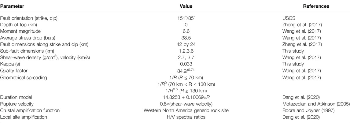
TABLE 1. Input parameters for the simulation of the Jiuzhaigou earthquake (Dang et al., 2020).

FIGURE 1

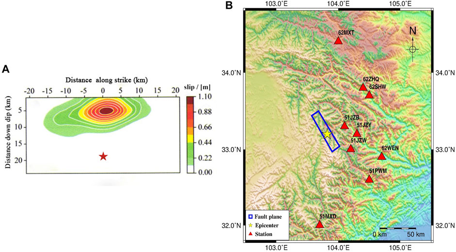
FIGURE 1. (A): Slip distribution of the Jiuzhaigou earthquake (Zheng et al., 2017) and (B): location of the fault plane and selected strong-motion stations. The black triangle indicates the stations triggered by the Jiuzhaigou earthquake, the red rectangle represents the fault plane, and the red pentagram represents the hypocenter.

TABLE 2

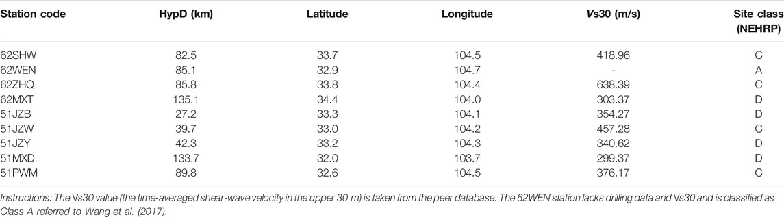
TABLE 2. Basic information of the strong motion observation stations in the Jiuzhaigou earthquake (Dang et al., 2020).

Path Duration Model

Husid (1969) suggested that the ground-motion energy that increases with time can be expressed in a formalized form as follows:

$I\left(t\right)=\frac{{\displaystyle {\int }_0^t{a}^2\left(t\right)dt}}{{\displaystyle {\int }_0^T{a}^2\left(t\right)dt}}(9)$

where T is the duration of the ground motion and I(t) denotes a function of 0–1.

As defined by Husid (1969), the effective duration was the time from the 5–95% Arias intensity instances, and the 90% ground-motion duration was observed to be I(t) = 0.05 and I(t) = 0.95.

In the present study, the duration function was directly derived from the robust regression of those effective durations determined based on 66 groups of recordings of strong earthquakes from the Jiuzhaigou earthquake, which is determined by T(R) = 14.8253 + 0.10669×R (Dang et al., 2020), where R denotes the epicentral distance (unit, km).

Attenuation Parameter

The high-frequency attenuation parameter κ is considered an important parameter that describes the decay of the acceleration Fourier amplitude spectrum of ground motion. The ground-motion amplitude at low frequencies, which is less than at the corner frequency, may be well described as a point source with an ω² shape (Aki, 1967; Brune, 1970). However, at high frequencies, the Fourier amplitude spectrum rapidly decreases when the frequency increases. Additionally, a significant difference is observed compared to the ω² spectrum. To describe this phenomenon, two filters are used to explain the diminution of high-frequency ground motions: the f_max filter (Boore, 1983; Hanks, 1982) and the κ₀ filter (Anderson and Hough, 1984). Certainly, both filters can be used individually in ground-motion simulations.

The main parameter needed in our applications is the zero-distance kappa factor, κ₀, gained from a best-fit line, which could be expressed in the form of κ = κ₀ + m×R, in which κ is the high-frequency attenuation parameter, κ₀ is the component related to the geological conditions below the station, and m is the component associated with the frequency-independent quality factor and the interlaminar shear-wave velocity. The Fourier amplitude spectrum is plotted in a semi-logarithmic coordinate system, considering the slope of the amplitude spectrum to be in the frequency range of a relatively smooth high spectrum, and the κ value of a single station is calculated by the formula, κ = k/(πlog10(e)), in which k is the slope and e is a natural constant. In this paper, the windowing function proposed by Konno and Ohmachi (1998) was employed for smoothing the obtained Fourier spectrum in a range of 0.5 and 15 Hz, while the smoothing constant was taken as 20 (Sun et al., 2013; Fu and Li, 2017; Kkallas et al., 2018). In our applications, we adopt the κ₀ filter in the form of κ = 0.033036 + 0.0008401×R, as shown in Figure 2, and employed the H/V spectral ratio approach (Lermo and Chávez-García, 1993) to estimate the local site amplification in the Jiuzhaigou earthquake (Dang et al., 2020).

FIGURE 2

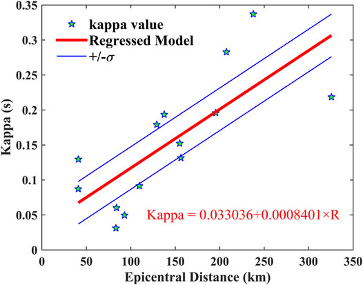
FIGURE 2. Dependence of spectral decay parameter κ on epicentral distance for horizontal component in the Jiuzhaigou earthquake. The light blue five-pointed star represents the kappa value obtained from each station recording, and the red solid line represents the regressed model.

Site Amplification

The amplification function used in stochastic simulation consists of two parts, namely, crustal amplification factors and the site amplification function. It is rarely sufficient to use crustal amplification factors if the station is located on a rock site. Otherwise, we are additionally required to use the site amplification function if the station is located on soil. In the case study of the Jiuzhaigou earthquake, we used both crustal site amplification (Table 3) and local site amplification functions, namely, the site amplification term is regarded as the combined action of crustal amplification and local site amplification. In the simulation, the crustal site amplification was determined according to the site classification of each station, and the local site amplification was obtained by H/V spectral ratio approach (Dang et al., 2020).

TABLE 3

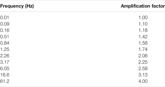
TABLE 3. Crustal site amplification elements used in the simulations (Boore and Joyner, 1997).

Northridge Earthquake

To make a better comparison, the Northridge earthquake (M_w 6.7) in 1994 was selected for illustration. Meanwhile, the dynamic and static corner frequencies (where the scaling factor H_ij was considered) were used for simulating the 15 stations that had an epicenter distance of <100 km. Figure 3A shows the distributions of the 15 selected stations. Then, at every station, the response spectra at the period of 0.05—10 s were determined. According to the National Earthquake Hazards Reduction Program (NEHRP) of the United States, the latitude and longitude of 15 stations, V_s30 (the average shear-wave velocity of 30 m below the surface), and the site classifications are presented in Table 4. The slip distribution of the Northridge earthquake used in this simulation is illustrated in Figure 3B (Wald et al., 1996). According to the source model given in Figure 3B, we divide the entire fault into several subfaults with a dimension of 3 km, and the slip amount of each subfault is shown in Figure 3C. The quality factors and the geometric attenuation model reference of Wang et al. (2015) are presented in Table 5. In addition, the static corner frequency of the Northridge earthquake calculated by Eq. 2 is 0.133 Hz, and the dynamic corner frequency of each subfault (△l = 3 km) calculated by Eq. 7 could be observed in Supplementary Table S2A.

FIGURE 3

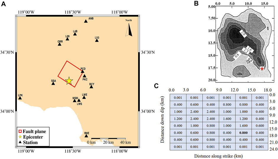
FIGURE 3. (A): Distribution of observation stations for the strong ground motion of the Northridge earthquake. The black triangle is the station triggered by the earthquake, and the red rectangle is the horizontal project of the fault; (B): source model of the Northridge earthquake (Wald et al., 1996; Sun, 2010; Dang et al., 2020); (C): slip amount of each subfault in the Northridge earthquake (Sun, 2010; Dang et al., 2020). The red star represents the hypocenter.

TABLE 4

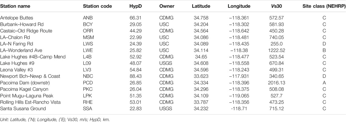
TABLE 4. Information on strong motion observation stations of the Northridge earthquake (Dang et al., 2020).

TABLE 5

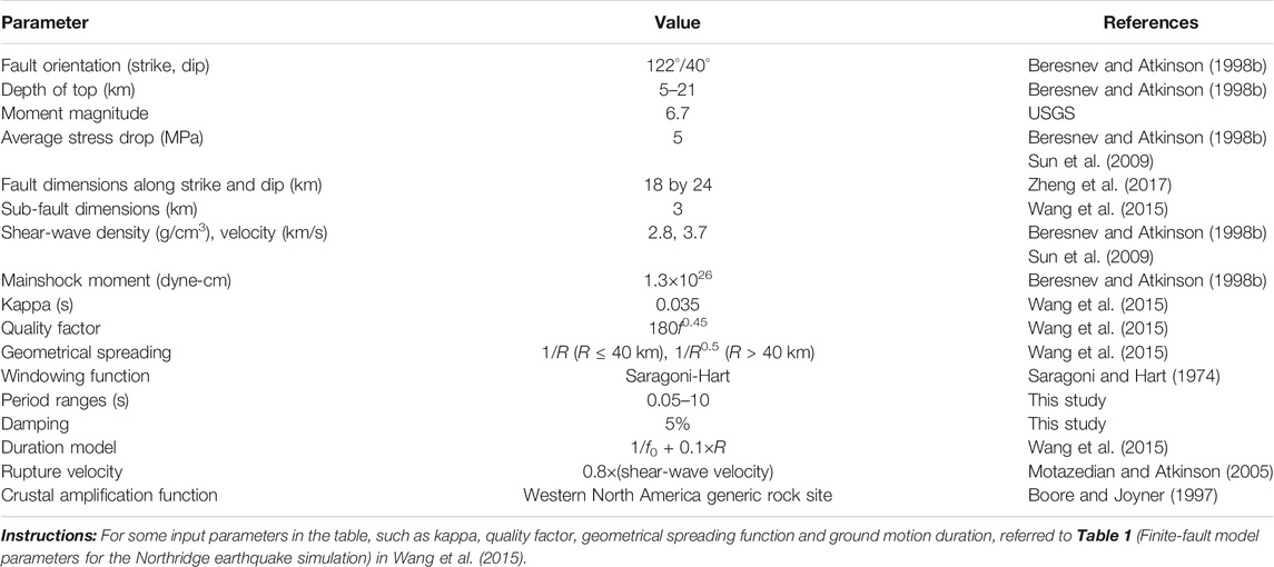
TABLE 5. Input parameters for the simulation of the Northridge earthquake.

Path Duration Model

The distance-dependent duration function used in the Northridge earthquake refers to Beresnev and Atkinson (1998b), which was found to be frequency dependent. In our implementations process, we used the duration function in the form of 0.1×R, where R denotes the epicentral distance in km. We attempted to apply dissimilar duration models for the Northridge earthquake. Unfortunately, none of the duration models used could significantly improve the simulation results. Finally, the duration model adopted in our study is in the form of T = 1/f₀ + 0.1×R (Wang et al., 2015). In addition, the high-frequency attenuation parameter, κ₀, is found to be 0.0035 (Wang et al., 2015).

Site Amplification

Since most of the 15 stations selected in the present study are located on sites class C, i.e., rock or stiff soil sites, for the sake of convenience, the site amplification factors for NEHRP-C sites were used for the site amplification of all stations, which is presented in Table 3.

Results and Discussion

Simulation Results of the Jiuzhaigou Earthquake

Comparison of the Far-Field Received Energy of the Jiuzhaigou Earthquake

The whole fault shown in Figure 1A is divided into rectangular subfaults of lengths 1, 2, 3, and 6 km, respectively. For subfaults of each length, we approximately estimate the slip amounts according to the slip color scale in Figure 1A. The slip distribution corresponding to each subfault length is shown in the supplementary materials, which can only be accessed through the network. The total far-field received energy of each subfault is found to be proportional to the square of the velocity spectrum. The far-field received energy of an observation point with an epicentral distance of 333 km is calculated by using the simulation parameters of the Jiuzhaigou earthquake as discussed above. The far-filed received energy calculated using the static corner frequency and the dynamic corner frequency is shown in Figures 4, 5, respectively. Obviously, Figures 4, 5 show that the far-field received energy calculated by the two corner frequencies is affected by the subfault size without considering the high-frequency scaling factor. Taking into account the high-frequency scaling factor H_ij, the far-field received energy obtained by the two corner frequencies no longer depends on the subfault size. Additionally, there is almost no difference in the far-field received energy between the two corner frequency models, which demonstrates that the use of the dynamic corner frequency itself does not eradicate the effect of the subfault size on the far-field received energy. The same result can be obtained by using the dynamic corner frequency and the static corner frequency. Although the corner frequency gradually decreases when the rupture process expands, the corner frequency of the subfault when the former rupture is always higher than that of the latter, and the corner frequency of the subfault where the rupture starting point is located is the largest. Sun et al. (2009), Wang et al. (2015), and other scholars have attempted to improve the source spectrum, but have never been able to ignore the influence of subfault size on the far-field received energy.

FIGURE 4

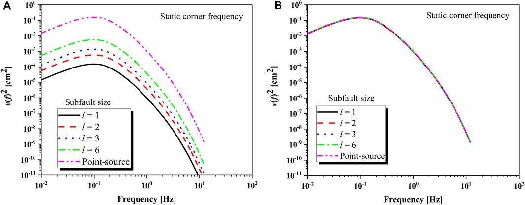
FIGURE 4. Far-field received energy calculated by the static corner frequency [(A): the scaling factor, H_ij, is not considered; (B): the scaling factor, H_ij, is considered]. The black solid line, red dotted line, blue dotted line, and pink dotted line indicate that the subfault sizes are 1, 2, 3, and 6, respectively. The pink dotted line represents the result obtained by stochastic point-source model.

FIGURE 5

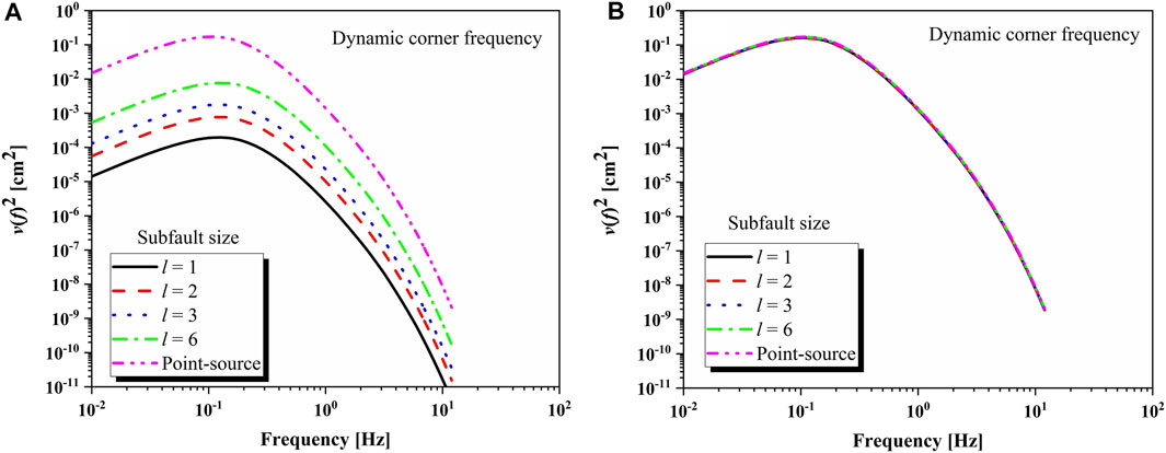
FIGURE 5. Far-field received energy calculated by the dynamic corner frequency [(A): the scaling factor, H_ij, is not considered; (B): the scaling factor, H_ij, is considered]. The black solid line, red dotted line, blue dotted line, and pink dotted line indicate that the subfault sizes are 1, 2, 3, and 6, respectively. The pink dotted line represents the result obtained by stochastic point-source model.

Comparison of Response Spectra of the Jiuzhaigou Earthquake

In addition, nine near-field stations with epicentral distance less than 150 km were selected, and the acceleration records of the nine near-field stations were simulated by the stochastic finite-fault method based on the improved static corner frequency and dynamic corner frequency. The results are shown in Figure 6. It can be seen in the figure that the SA obtained by the static corner frequency (where the scaling factor H_ij was considered) and the dynamic corner frequency model are in good agreement with the observed SA. Meanwhile, the response spectra obtained by the two models have little difference, especially for stations 62WEN, 62ZHQ, 62MXT, 62SHW, 51JZW, and 51PWM. At the same time, Figure 6B shows that the PGAs of the nine stations simulated by the two corner frequency models are similar, and they are in good agreement with the observed PGAs. It should be noted that the simulated PGA is the average results of 30 runs of the program. This result shows that the static corner frequency with a high-frequency scaling factor can also obtain ideal results and that the influence of subfault size can be ignored.

FIGURE 6

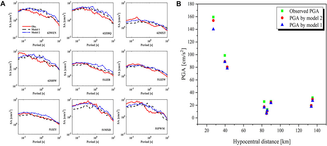
FIGURE 6. (A) Comparison of the observed and simulated SA for the nine stations in the Jiuzhaigou earthquake; (B) Comparison of observed, simulated PGA values by the two corner frequency models. Simulated SAs and PGAs are the average of 30 trials for each case. The red solid line represents the observed SA. The black dashed line and the blue dashed line represent the simulated SA obtained by the static corner frequency (Model 1) and the dynamic corner frequency (Model 2), respectively. The green rectangle stands for the observed PGA. The red circle and blue triangle represent the PGA simulated by the dynamic and static corner frequency models, respectively.

Simulation Results of the Northridge Earthquake

Comparison of the Simulated Response Spectra of the Northridge Earthquake

The stochastic finite-fault approach was adopted to calculate the SA of 15 stations based on the static and dynamic corner frequencies, which were then compared with those obtained by observation recordings. The results are presented in Figure 7, which shows that for most stations, the results of the two models are in good agreement with the observation recordings, especially at the LWE, L4B, LV3, PKC, PCD, ANB, and RHE stations. However, for the SSA and MSM stations, considerable differences were observed in response spectra for long periods. As shown in Figure (a), the MSM and SSA stations were located at the fault edge, and both of them had an epicentral distance of <23 km. This might be due to the impacts of directivity, including forward and backward effects. The forward effect takes place at the time of the front propagation of rupture to a site, inducing great ground-motion amplitudes and low duration compared with those under mean directivity situations. In contrast, the backward effect takes place at the time of propagation of rupture from a site that produces low amplitudes and long duration motions in the long term (Sun, 2010). The ORR station had undervalued response spectra nearly during the whole period, which conformed to the results obtained by Beresnev and Atkinson (1998b) and Sun et al. (2009). The reasons for these differences may be attributed to the fact that the selected site amplification factor fail to describe the local geological conditions, which may require complete site data for analysis. Generally, the results of the two models do not show many differences.

FIGURE 7

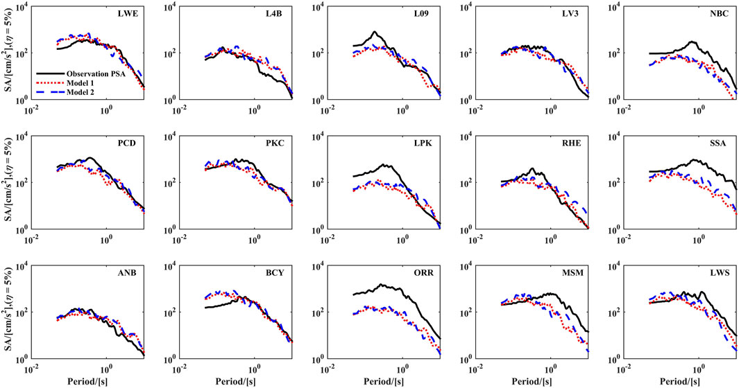
FIGURE 7. Comparison of the observed and the simulated SA for the 15 selected stations in the Northridge earthquake. Simulated SAs are the average of 30 trials for each case. The black solid line represents the observed SA. The red dashed line and the blue double dashed line represent the simulated SA obtained by the static corner frequency (Model 1) and the dynamic corner frequency (Model 2), respectively.

Validation of the Stochastic Finite-Fault Approach

Given the abovementioned concluded model parameters, for the 15 stations involved in the Northridge earthquake, the stochastic finite-fault method was used to calculate their 5%-damped acceleration response spectra based on the dynamic and static corner frequencies (range: 0.05–10 s). In the frequency domain, the model bias function (B(f)) is defined as follows (Somerville et al., 1997; Dang and Liu, 2020):

$r{\left(f\right)}_{ij}=\log \left(\frac{SA{\left(f\right)}_{ij}^{Simulated}}{SA{\left(f\right)}_{ij}^{Observed}}\right)(10)$

$B_i\left(f\right)=\frac{1}{N}{\displaystyle \sum _{j=1}^N{r}_{ij}\left(f\right)}(11)$

where N denotes the number of stations; $SA{\left(f\right)}_{ij}^{Simulated}$ and $SA{\left(f\right)}_{ij}^{Observed}$ represent the simulated SA values and the observed SA values of the ith station at the jth frequency, respectively. The period range is 0.05–10 s. Figure 8 shows plots of the model bias for the two models.

FIGURE 8

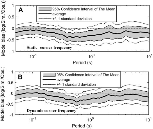
FIGURE 8. Model bias [log(SA^Simulated)—log(SA^Observed)) and standard deviation for the 15 stations in the Northridge earthquake calculated by the static corner frequency and the dynamic corner frequency, respectively; (A) the static corner frequency; (B) the dynamic corner frequency.

Similarly, the standard deviation of the model is defined as follows (Castro et al., 2008):

${\sigma }_i\left(f\right)=\sqrt{\frac{1}{N}{\displaystyle \sum _{j=1}^N{\left[r_{ij}\left(f\right)-B_i\left(f\right)\right]}^2}}(12)$

Table 6 presents the model standard deviation of the 15 stations, which are calculated using the dynamic corner frequency and the static corner frequency. Obviously, although the model bias of the nine stations calculated by using the dynamic corner frequency is small, the model deviations of each station calculated by using the two corner frequencies are not much different. Additionally, the average values differ by only 0.01.

TABLE 6

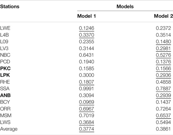
TABLE 6. The average errors computed at each station: the underlined values display the minimum error values. The bold characters indicate that there is little difference between the results of the two models.

Finally, we applied an additional measure of the misfit (E_j), where the absolute value is taken inside the summation over stations in the expression for the bias and the average absolute error (E) indicates the absolute differences between the simulated SA and the observed SA averaged over the selected 15 stations and the frequency range of engineering interest based on the following equations (Schneider et al., 1993):

$E_j=\frac{1}{N}{\displaystyle \sum _{i=1}^{N}ABS\left\{\log A_{ij}^{Observed}-\log A_{ij}^{Simulated}\right\}}(13)$

$E=\frac{1}{K}{\displaystyle \sum _{j=1}^K{E}_j}(14)$

where ABS indicates the absolute value; N is the number of stations; K is the number of frequencies; $A_{ij}^{Observed}$ and $A_{ij}^{Simulated}$ are the observed SA and the simulated SA of the ith station at the jth frequency, respectively; and E_j represents the average absolute error of a station at the jth frequency. The average absolute error for the two models is presented in Table 7.

TABLE 7

TABLE 7. The average absolute error for the two models.

According to Table 7, the average absolute error of the models calculated by using the two models is not much different, which indicates that both models can obtain ideal results when simulating the ground motion.

Conclusion

In the present work, the stochastic finite-fault approach is used on the basis of the dynamic and static corner frequencies for simulating the 15 stations involved in the Northridge earthquake (M_w 6.7) that occurred in 1994 in the United States. The total spectral ratio, model bias, and the total model error of the two models are calculated separately. In addition, the results of the two models are similar. In the case of a few stations, the simulated results of the two models are significantly different from the observed results, which is found to be consistent with the results obtained by Sun et al. (2009) and Beresnev and Atkinson (1998b). These differences may be caused by local site effects, topography, and basin geometry effects, which may require complete site data for analysis. According to the simulated results of the two stations (PCD and SSA), the directivity effect induces a great influence on the amplitude of SA. The reason is that the epicentral distance of the two stations are almost the same (Figure 3A; Table 4), and they are located at the upside and downward positions of the fault, respectively. Additionally, the response spectra, average spectral ratio, model deviation, and average absolute error of the 15 stations with an epicentral distance of less than 100 km of the Northridge earthquake (M_w 6.7) in the United States are also calculated. Based on the results, little difference is observed between the two models.

The far-field received energy of the Jiuzhaigou earthquake (M_w 6.6) that occurred in 2017 with an epicentral distance of 333 km is calculated by the stochastic finite-fault method based on the static corner frequency and the dynamic corner frequency. When the high-frequency scaling factor and the filter function are not considered, the far-field received energy obtained by the two models depends on the size of the subfault. After modification, the far-field received energy calculated by the two models becomes independent of the size of the subfault. In the literal sense, the subfault corner frequency primarily depends on the rupture order and the subfault corner frequency. As the rupture expands, the corner frequency gradually decreases. At high frequencies, the Fourier amplitude spectrum is positively correlated with the square of the corner frequency. As a result, the high frequency spectrum amplitude is underestimated. During the propagation of the rupture to each subfault onto the major fault, the subfault corner frequency reaches the lower limit. This is called the static corner frequency for the entire fault and is the underestimated corner frequency (Sun et al., 2009; Wang et al., 2015). Consequently, the high-frequency received energy and the level spectrum are significantly underestimated. In addition, the scaling factor at high frequencies is determined according to the mean received energy distribution to every subfault, and it cannot represent the slip distribution impact on the far-field received energy. According to Eq. 8, the scaling factor of every subfault can be obtained on the basis of the calculated far-field received energy by using the whole fault corner frequency and the seismic moment of every subfault, which shows a strong correlation with the subfault number. In reality, the physical explanation of a changing corner frequency with an additional subfault is called the growth of the rupture. An earthquake ruptures over time, where both the area of the rupture and the seismic moment increase with time. Although a subfault is supposed only to represent a small portion of the fault, an increase in the corner frequency with time ideally replicates the rupture growth with time. This explains the change in the subfault corner frequency with time other than the order of its rupture. Finally, the conclusions of this study also confirm that the stochastic finite-fault method based on static corner frequency can be applied to practical engineering with the addition of a high-frequency scaling factor, and the dependence of the simulation results on the size of the subfault is very small or even negligible.

Although we make corrections to FINSIM, such as adding high-frequency scaling factor and correcting the calculation of corner frequency and seismic moment, these corrections make the simulation results independent of subfault size and basically consistent with the simulation results of EXSIM. However, it also shows that the dynamic corner frequency itself has many disadvantages. No matter how the corner frequency is defined, the spectral amplitude is adjusted by the high-frequency scaling factor. In the dynamic corner frequency, the corner frequency of the subfault is only related to its rupture order. The corner frequency of the subfault that breaks first is greater than that of the subfault that breaks later, which obviously dose not conform to the ground motion characteristics. In the calculation of high-frequency scaling factor, it is assumed that the seismic moments of each subfault are equal, which cannot fully explain the influence of uneven distribution of dislocation on the high-frequency scaling factor. Therefore, the stochastic finite-fault approach still needs further research to meet the engineering needs.

Data Availability Statement

The original contributions presented in the study are included in the article/Supplementary Material, further inquiries can be directed to the corresponding author.

Author Contributions

PD carried out the theoretical studies including conception and design, material preparation, data collection, and was a major contributor in writing the manuscript. PD and QL analyzed the conclusion. LJ collected the data. All authors read and approved the final manuscript.

Funding

This research was undertaken with the support of the National Natural Science Foundation of China under Grant Nos. 52020105002, 51878192, 51978434, 52011530394, and 51991393.

Conflict of Interest

Author LJ was employed by Central and Southern China Municipal Engineering Design and Research Institute Co., Ltd.

The remaining authors declare that the research was conducted in the absence of any commercial or financial relationships that could be construed as a potential conflict of interest.

Publisher’s Note

All claims expressed in this article are solely those of the authors and do not necessarily represent those of their affiliated organizations, or those of the publisher, the editors and the reviewers. Any product that may be evaluated in this article, or claim that may be made by its manufacturer, is not guaranteed or endorsed by the publisher.

Acknowledgments

We thanks David Boore for providing the EXSIM code. Thank Song Jian and Ligang Feng, Institute of Engineering Mechanics, China Earthquake Administration, for his help in drawing picture using Generic Mapping Tools (GMT) software (https://gmt-china.org/example/). Finally, we thank AJE (https://www.aje.com/) for its linguistic assistance during the preparation of this manuscript. At last but not least, we would like to thank two reviewers for the helpful comments and suggestions.

Supplementary Material

The Supplementary Material for this article can be found online at: https://www.frontiersin.org/articles/10.3389/feart.2021.813089/full#supplementary-material

References

Aki, K., and Richards, P. (1980). Quantitative Seismology: Theory and Method. San Francisco: W. H. Freeman and Company, 932.

Google Scholar

Aki, K. (1967). Scaling Law of Seismic Spectrum. J. Geophys. Res. 72, 1217–1231. doi:10.1029/jz072i004p01217

CrossRef Full Text | Google Scholar

Anderson, J. G., and Hough, S. E. (1984). A Model for the Shape of the Fourier Amplitude Spectrum of Acceleration at High Frequency. Bull. Seismological Soc. America 74, 1969–1993. doi:10.1785/bssa0740030995

CrossRef Full Text | Google Scholar

Beresnev, I. A., and Atkinson, G. M. (1998a). FINSIM--a FORTRAN Program for Simulating Stochastic Acceleration Time Histories from Finite Faults. Seismological Res. Lett. 69, 27–32. doi:10.1785/gssrl.69.1.27

CrossRef Full Text | Google Scholar

Beresnev, I. A., and Atkinson, G. M. (1998b). Stochastic Finite-Fault Modeling of Ground Motion from the 1994 Northridge, California, Earthquake. 1. Validation on Rock Sites. Bull. Seismological Soc. America 88, 1392–1401. doi:10.1785/bssa0880041079

CrossRef Full Text | Google Scholar

Boore, D. M. (2009). Comparing Stochastic point-source and Finite-Source Ground-Motion Simulations: SMSIM and EXSIM. Bull. Seismological Soc. America 99, 3202–3216. doi:10.1785/0120090056

CrossRef Full Text | Google Scholar

Boore, D. M., and Joyner, W. B. (1997). Site Amplifications for Generic Rock Sites. Bull. Seismological Soc. America 87 (2), 327–341. doi:10.1785/bssa0870020327

CrossRef Full Text | Google Scholar

Boore, D. M. (2003). Simulation of Ground Motion Using the Stochastic Method. Pure Appl. Geophys. 160, 635–676. doi:10.1007/pl00012553

CrossRef Full Text | Google Scholar

Boore, D. M. (1983). Stochastic Simulation of High-Frequency Ground Motions Based on Seismological Models of the Radiated Spectra. Bull. Seismological Soc. America 73, 1865–1894.

Google Scholar

Boore, D. M., and Thompson, E. M. (2015). Revisions to Some Parameters Used in Stochastic‐Method Simulations of Ground Motion. Bull. Seismological Soc. America 105, 1029–1041. doi:10.1785/0120140281

CrossRef Full Text | Google Scholar

Brune, J. N. (1970). Tectonic Stress and the Spectra of Seismic Shear Waves from Earthquakes. J. Geophys. Res. 75, 4997–5009. doi:10.1029/jb075i026p04997

CrossRef Full Text | Google Scholar

Castro, R. R., Pacor, F., Franceschina, G., Bindi, D., Zonno, G., and Luzi, L. (2008). Stochastic Strong-Motion Simulation of the Mw 6 Umbria-Marche Earthquake of September 1997: Comparison of Different Approaches. Bull. Seismological Soc. America 98, 662–670. doi:10.1785/0120070092

CrossRef Full Text | Google Scholar

Chopra, S., Kumar, D., Choudhury, P., and Yadav, R. B. S. (2012). Stochastic Finite Fault Modelling of M W 4.8 Earthquake in Kachchh, Gujarat, India. J. Seismol 16, 435–449. doi:10.1007/s10950-012-9280-0

CrossRef Full Text | Google Scholar

Dang, P., Liu, Q., and Song, J. (2020). Simulation of the Jiuzhaigou, China, Earthquake by Stochastic Finite-Fault Method Based on Variable Stress Drop. Nat. Hazards 103 (2), 2295–2321. doi:10.1007/s11069-020-04083-9

CrossRef Full Text | Google Scholar

Dang, P., and Liu, Q. (2020). Stochastic Finite-Fault Ground Motion Simulation for the Mw 6.7 Earthquake in Lushan, China. Nat. Hazards 100 (3), 1215–1241. doi:10.1007/s11069-020-03859-3

CrossRef Full Text | Google Scholar

Dang, P., Liu, Q., Xia, S., and Ma, W. (2021). A Stochastic Method for Simulating Near‐Field Seismograms: Application to the 2016 Tottori Earthquake. Earth Space Sci. 8 (11), e2021EA001939. doi:10.1029/2021EA001939

CrossRef Full Text | Google Scholar

Frankel, A. (2009). A Constant Stress-Drop Model for Producing Broadband Synthetic Seismograms: Comparison with the Next Generation Attenuation Relations. Bull. Seismological Soc. America 99, 664–680. doi:10.1785/0120080079

CrossRef Full Text | Google Scholar

Fu, L., and Li, X. J. (2017). The Kappa (κ₀) Model of the Longmenshan Region and its Application to Simulation of strong Ground-Motion by the Wenchuan Ms 8.0 Earthquake. Chin. J. Geophys. 60 (8), 2935–2947. doi:10.6038/cjg20170803

CrossRef Full Text | Google Scholar

Graves, R. W., and Pitarka, A. (2010). Broadband Ground-Motion Simulation Using a Hybrid Approach. Bull. Seismological Soc. America 100, 2095–2123. doi:10.1785/0120100057

CrossRef Full Text | Google Scholar

Graves, R. W., and Pitarka, A. (2004). “Broadband Time History Simulation Using a Hybrid Approach,” in Proceeding of the 13th world Conference on Earthquake Engineering 2004, Vancouver, Canada, August 6-1, 2004.

Google Scholar

Hanks, T. C. (1982). f max. Bull. Seismological Soc. America 72, 1867–1879. doi:10.1785/bssa07206a1867

PubMed Abstract | CrossRef Full Text | Google Scholar

Hartzell, S. H. (1978). Earthquake Aftershocks as Green's Functions. Geophys. Res. Lett. 5, 1–4. doi:10.1029/gl005i001p00001

CrossRef Full Text | Google Scholar

Husid, R. L. (1969). Analisis de terremotos: Analisi general. Revista. Del. IDIEM 8, 21–42.

Google Scholar

Kkallas, C. C. B., Papazachos, C. B., Margaris, B. N., Boore, D., Ventouzi, C., and Skarlatoudis, A. (2018). Stochastic Strong Ground Motion Simulation of the Southern Aegean Sea Benioff Zone Intermediate‐Depth Earthquakes. Bull. Seismological Soc. America 108 (2), 946–965. doi:10.1785/0120170047

CrossRef Full Text | Google Scholar

Konno, K., and Ohmachi, T. (1998). Ground-motion Characteristics Estimated from Spectral Ratio between Horizontal and Vertical Components of Microtremor. Bull. Seismological Soc. America 88 (1), 228–241. doi:10.1785/bssa0880010228

CrossRef Full Text | Google Scholar

Lermo, J., and Chávez-García, F. J. (1993). Site Effect Evaluation Using Spectral Ratios with Only One Station. Bull. Seismological Soc. America 83, 1574–1594. doi:10.1785/bssa0830051574

CrossRef Full Text | Google Scholar

Mavroeidis, G. P., and Papageorgiou, A. S. P. (2003). A Mathematical Representation of Near-Fault Ground Motions. Bull. Seismological Soc. America 93, 1099–1131. doi:10.1785/0120020100

CrossRef Full Text | Google Scholar

Motazedian, D., and Atkinson, G. M. (2005). Stochastic Finite-Fault Modeling Based on a Dynamic Corner Frequency. Bull. Seismological Soc. America 95, 995–1010. doi:10.1785/0120030207

CrossRef Full Text | Google Scholar

Motazedian, D., and Moinfar, A. (2006). Hybrid Stochastic Finite Fault Modeling of 2003, M6.5, Bam Earthquake (Iran). J. Seismol 10, 91–103. doi:10.1007/s10950-005-9003-x

CrossRef Full Text | Google Scholar

Raghu Kanth, S. T. G., and Kavitha, B. (2013). Stochastic Finite Fault Modeling of Subduction Zone Earthquakes in Northeastern India. Pure Appl. Geophys. 170, 1705–1727. doi:10.1007/s00024-012-0622-1

CrossRef Full Text | Google Scholar

Saragoni, G. R., and Hart, G. C. (1974). Simulation of Artificial Earthquake. Earthquake Eng. Struct. Dyn. 2, 249–267.

Google Scholar

Schneider, J. F., Silva, W. J., and Stark, C. (1993). Ground Motion Model for the 1989 M 6.9 Loma Prieta Earthquake Including Effects of Source, Path, and Site. Earthquake Spectra 9, 251–287. doi:10.1193/1.1585715

CrossRef Full Text | Google Scholar

Sharma, N., Srinagesh, D., Suresh, G., and Srinivas, D. (2021). Stochastic Simulation of Strong Ground Motions from Two M > 5 Uttarakhand Earthquakes. Front. Earth Sci. 9, 599535. doi:10.3389/feart.2021.599535

CrossRef Full Text | Google Scholar

Somerville, P. G., Smith, N. F., Graves, R. W., and Abrahamson, N. A. (1997). Modification of Empirical strong Ground Motion Attenuation Relations to Include the Amplitude and Duration Effects of Rupture Directivity. Seismological Res. Lett. 68, 199–222. doi:10.1785/gssrl.68.1.199

CrossRef Full Text | Google Scholar

Sun, X. D. (20102010). Research on Several Problems in Estimation of strong Earthquake Field. China: Harbin Institute of Technology.

Google Scholar

Sun, X., Tao, X., Duan, S., and Liu, C. (2013). Kappa (K) Derived from Accelerograms Recorded in the 2008 Wenchuan Mainshock, Sichuan, China. J. Asian Earth Sci. 73, 306–316. doi:10.1016/j.jseaes.2013.05.008

CrossRef Full Text | Google Scholar

Sun, X., Tao, X., Wang, G., and Liu, T. (2009). Dynamic Corner Frequency in Source Spectral Model for Stochastic Synthesis of Ground Motion. Earthq Sci. 22, 271–276. doi:10.1007/s11589-009-0271-3

CrossRef Full Text | Google Scholar

Sutar, A. K., Verma, M., Bansal, B. K., and Pandey, A. P. (2020). Simulation of strong Ground Motion for a Potential Mw7.3 Earthquake in Kopili Fault Zone, Northeast India. Nat. Hazards 104, 437–457. doi:10.1007/s11069-020-04176-5

CrossRef Full Text | Google Scholar

Tanırcan, G., and Yelkenci-Necmioğlu, S. (2020). Simulation of the strong Ground Motion for the 20 July 2017 (Mw. 6.6) Bodrum–Kos Earthquake. Bull. Earthquake Eng. 18 (13), 5807–5825. doi:10.1007/s10518-020-00892-2

CrossRef Full Text | Google Scholar

Toni, M. (2017). Simulation of strong Ground Motion Parameters of the 1 June 2013 Gulf of Suez Earthquake, Egypt. NRIAG J. Astron. Geophys. 6, 30–40. doi:10.1016/j.nrjag.2016.12.002

CrossRef Full Text | Google Scholar

Wald, D. J., Heaton, T. H., and Hudnut, K. W. (1996). The Slip History of the 1994 Northridge, California, Earthquake Determined from strong-motion, Teleseismic, GPS, and Leveling Data. Bull. Seismological Soc. America 86, S49–S70. doi:10.1785/bssa08601b0s49

CrossRef Full Text | Google Scholar

Wang, G., Ding, Y., and Borcherdt, R. (2015). Simulation of Acceleration Field of the Lushan Earthquake (Ms7.0, April 20, 2013, China). Eng. Geology. 189, 84–97. doi:10.1016/j.enggeo.2015.02.003

CrossRef Full Text | Google Scholar

Wang, H. W., Ren, Y. F., and Wen, R. Z. (2017). Source Spectra of the 8 August 2017 Jiuzhaigou Ms7.0 Earthquake and the Quality Factor of the Epicenter Area. Chin. J. Geophys. 60, 4117–4123. doi:10.6038/cjg20171036

CrossRef Full Text | Google Scholar

Zafarani, H., Rahimi, M., Noorzad, A., Hassani, B., and Khazaei, B. (2015). Stochastic Simulation of Strong‐Motion Records from the 2012 Ahar-Varzaghan Dual Earthquakes, Northwest of Iran. Bull. Seismological Soc. America 105, 1419–1434. doi:10.1785/0120140241

CrossRef Full Text | Google Scholar

Zheng, X. J., Zhang, Y., and Wang, R. J. (2017). Estimating the Rupture Process of the 8 August 2017 Jiuzhaigou Earthquake by Inverting strong-motion Data with IDS Method. Chin. J. Geophys. 60, 4421–4430. doi:10.6038/cjg20171128

CrossRef Full Text | Google Scholar