Daily Runoff Forecasting Using Ensemble Empirical Mode Decomposition and Long Short-Term Memory

Hydrological series data are non-stationary and nonlinear. However, certain data-driven forecasting methods assume that streamflow series are stable, which contradicts reality and causes the simulated value to deviate from the observed one. Ensemble empirical mode decomposition (EEMD) was employed in this study to decompose runoff series into several stationary components and a trend. The long short-term memory (LSTM) model was used to build the prediction model for each sub-series. The model input set contained the historical flow series of the simulation station, its upstream hydrological station, and the historical meteorological element series. The final input of the LSTM model was selected by the MI method. To verify the effect of EEMD, this study used the Radial Basis Function (RBF) model to predict the sub-series, which was decomposed by EEMD. In addition, to study the simulation characteristics of the EEMD-LSTM model for different months of runoff, the GM(group by month)-EEMD-LSTM was set up for comparison. The key difference between the GM-EEMD-LSTM model and the EEMD-LSTM model is that the GM model must divide the runoff sequence on a monthly basis, followed by decomposition with EEMD and prediction with the LSTM model. The prediction results of the sub-series obtained by the LSTM and RBF exhibited better statistical performance than those of the original series, especially for the EEMD-LSTM. The overall GM-EEMD-LSTM model performance in low-water months was superior to that of the EEMD-LSTM model, but the simulation effect in the flood season was slightly lower than that of the EEMD-LSTM model. The simulation results of both models are significantly improved compared to those of the LSTM model.

Introduction

The Three Gorges Reservoir is located in the upper reaches of the Yangtze River. The Three Gorges Project is the largest water conservancy project in the world. It plays an important role in the governance and development of the Yangtze River and has comprehensive benefits such as flood control, hydropower generation, and increased water supply (News and Focus, 2015). Forecasting Three Gorges River inflows is critical for dispatching cascaded hydropower stations for optimal production and operation. Accurate hydrological forecasts are not beneficial for deciding the optimal dispatch time and reservoir station locations, but they are conducive to the development and adjustment of station power generation plans (Cheng et al., 2015). Two primary types of runoff prediction methods have been developed: physical analysis models and data-driven methods. Physical models are based on the hydrological dynamic process, and they are closely integrated with the spatio-temporal precipitation distribution, meteorological conditions, and underlying surface conditions (Lee et al., 2020). Zhu et al. (2019) proposed a method to improve runoff simulation by fusing multi-source precipitation products. Patil and Ramsankaran (2017) improved the flow simulation and prediction performance of the Soil and Water Assessment Tool (SWAT) by assimilating remotely sensed soil moisture observations. Due to the high data requirements of physical analysis models and the complexity of runoff generation and flow concentration processes, it is difficult to establish precise hydrological models, which restricts the application of physical models. Therefore, scholars have utilized data-driven methods to solve these problems (Abbaspour et al., 2015; Wang et al., 2018).

Data-driven methods rely on historical observation data to predict data characteristics and the relationship between model inputs and outputs. Data-driven methods have been widely used and have achieved excellent results (Kan et al., 2016). Wu et al. (2005) developed an artificial neural network (ANN) model and successfully applied it to short-term flow forecasting. Nanda et al. (2016) used a linear autoregressive moving average model to forecast floods with a forecast period of 1 d–3 days Ahmadi et al., 2019 used ANN models on a daily, monthly, and annual basis in the Kan watershed, which is located in western Tehran, Iran. Certain data-driven forecasting methods, such as the ANN, adaptive-network-based fuzzy inference system, and support vector machine methods assume that streamflow series are stable, which contradicts reality and causes the simulated value to deviate from the observed one (Adamowski et al., 2014).

In order to solve the instability problem of the runoff series and improve the simulation accuracy of model, many studies employed ensemble empirical mode decomposition (EEMD) to process the runoff series and decompose the non-stationary original series into a trend with several stable sub-series. This method has been widely used in combination with data-driven methods in recent years. Tan et al. (2018) used an EEMD-ANN model to forecast the monthly runoff at three stations in Ertan, Cuntan, and Yichang. Wang et al. (2020) used ANN and SVR to regress a monthly flow series decomposed by EEMD according to the climate index.

The EEMD is an optimized version of empirical mode decomposition (EMD) method. Huang et al. (1998) proposed the EMD method in 1998. The EMD method innovatively introduces “intrinsic mode functions” based on the local characteristics of the signal, which makes the instantaneous frequency meaningful. This makes it suitable for nonlinear and linear stationary processes. The final results of EMD decomposition are reflected in an energy-frequency-time distribution (Huang et al., 1998). Zhao et al. (2017) used the EMD method to decompose annual runoff; they effectively improved the simulation accuracy of the Chaotic Least Squares Support Vector Machine model. Based on EMD, the EEMD method improves the phenomenon of EMD modal aliasing by adding white noise. It can add white noise without any basic function, so that signals with different scales can be clearly sorted in the appropriate intrinsic mode function (IMF) (Huang and Wu, 2008). Wang et al. (2015) used the EEMD method to decompose an annual runoff sequence, and constructed an EEMD-ANN model. Their results showed that the EEMD method effectively improved the simulation performance of their ANN. Yu et al. (2018) combined the EEMD method with a radial basis function (RBF) neural network and an autoregression (AR) model to forecast annual runoff, effectively improving the simulation accuracies of the two models.

Combining EEMD and data-driven methods for data series prediction has been extensively studied in various fields, but few studies combine the EEMD and long short-term memory (LSTM) methods or use these combined methods to perform runoff predictions. Zhang et al. (2018) used the EEMD-LSTM method to predict the daily surface temperature, comparing it with the EMD-LSTM and EEMD-RNN methods and demonstrating that the EEMD-LSTM model is the most suitable tool for temperature prediction. An et al. (2020) used singular spectrum analysis (SSA) and EEMD to extract the frequency and trend features of Niangziguan spring discharge, and then they used LSTM to simulate each frequency and trend sub-sequence. The results demonstrate that the SSA-LSTM and EEMD-LSTM performances are superior to that of LSTM, and the EEMD-LSTM model achieved the optimal prediction performance. Therefore, this study utilizes LSTM to determine whether runoff data processed by EEMD can improve the prediction performance of the LSTM model for runoff data. In addition, this study utilized the mutual information method which is suitable for handling the nonlinear relationship between hydrological series to select the input variables.

The remainder of this paper is organized as follows. Materials and Method contains the methods used in the research and relevant information about the study area, model inputs, parameter settings, and verification strategy. Results and Discussion describes the calculation results and analysis of each step, and Conclusion contains the research conclusions.

Materials and Methods

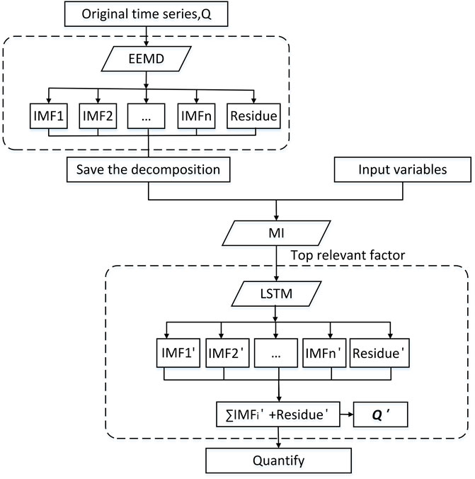
The main purpose of this research is to study whether the data processed by EEMD can improve the simulation performance of the LSTM model for runoff data. Therefore, the main structure of the model is decomposition-analysis-simulation, as shown in Figure 1.

FIGURE 1

FIGURE 1. Research flowchart.

EEMD

EEMD optimizes EMD, improving the mode mixing phenomenon of EMD by adding white noise. The EEMD method adds the appropriate amount of white noise to the original sequence and then divides the original sequence into a trend and n finite intrinsic mode functions (IMFs) (Huang and Wu, 2008; Wang et al., 2020). The specific EEMD steps are as follows:

1 Step 1: Input the data to be decomposed as the original signal x(t) and set the EEMD parameters, including the noise standard deviation (Nstd), number of realizations (NR), and maximum number of sifting iterations allowed (MaxIter).

2 Step 2: Add white noise (wi(t)) to the original sequence to form the following new sequence:

$x_i\left(t\right)=x\left(t\right)+w_i\left(t\right)(1)$

3 Step 3: Using the following formula, EMD divides the new sequence obtained in Step 2 into n finite IMFs and a trend item.

$x_i\left(t\right)={\displaystyle \sum _{j=1}^n{c}_{ij}}\left(t\right)+r_i\left(t\right)(2)$

4 Step 4: Repeat Steps 2 and 3 until the maximum NR is achieved for i.

5 Step 5: IMFs are calculated using Eq. 3, and the final result is obtained using Eq. 4.

$c_j\left(t\right)={\displaystyle \sum _{i=1}^{NR}cij\left(t\right)}/NR(3)$

$x\left(t\right)={\displaystyle \sum _{j=1}^n{c}_j}\left(t\right)+r\left(t\right)(4)$

where cj(t) represents the jth IMF, and r(t) is the trend item.

Mutual Information

The mutual information method describes the degree of correlation between two random variables, and it can reflect both the non-linear and linear correlations. If variables x and y are related, and x is known, the uncertainty of y can be reduced according to the degree of mutual information between x and y. If variables x and y are independent of each other, the joint density is equal to the product of their edge distribution density (Sharma, 2000; Zhao and Yang, 2011; Ding et al., 2019), which can be expressed as follows:

$P_{x,y}(x,y)=P_x\left(x\right)P_y\left(y\right)(5)$

When variables x and y have N observations and are discrete random variables, the mutual information between the variables can be expressed as follows:

$MI=\frac{1}{N}{\displaystyle \sum _{i=1}^{N}Ln[\frac{P_{x,y}(x_i,y_i)}{P_x\left(x_i\right)P_y\left(y_i\right)}}](6)$

When the variables x and y are continuous random variables, the mutual information equation between the variables is

$MI={\displaystyle \iint \mu (x,y)Lg}\frac{\mu (x,y)}{{\mu }_x\left(x\right){\mu }_y\left(y\right)}dxdy(7)$

where µ(x,y) represents the joint distribution density of continuous random variables x and y; and µ_x(x) and µ_y(y) represent the marginal distribution densities of continuous random variables x and y, respectively.

When the random variables x and y are independent of each other, $L\text{n}\left[\frac{P_{x,y}(x_i,y_i)}{P_x\left(x_i\right)P_y\left(y_i\right)}\right]=0$, and $L\text{g}\frac{\mu (x,y)}{{\mu }_x\left(x\right){\mu }_y\left(y\right)}=0$, then MI = 0. When x and y are not independent of each other, MI approaches positive infinity.

Long Short-Term Memory

LSTM is an improved recurrent neural network (RNN) that resolves the problem of gradient disappearance during an RNN simulation. LSTM replaces the cell unit in the RNN with a memory unit, which effectively improves the long-term memory ability of the neural network (Kratzert et al., 2018). LSTM is connected in a time sequence. At time t, the input of the memory unit includes the hidden layer state variable h_t−1 at time t₋1 and the state variable C_t−1 of the memory unit and input information x_t at time t. Additionally, the forget gate f_t, input gate i_t, and output gate o_t are coordinately controlled. Finally, the calculation result y_t of the LSTM at time t is obtained, and it is passed into the calculation at time t+1 together with C_t (Yin et al., 2019). The LSTM memory unit structure is displayed in Figure 2.

FIGURE 2

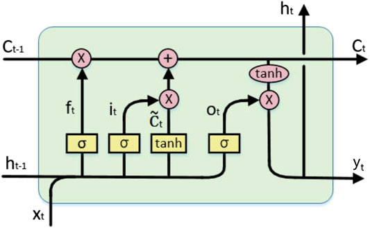
FIGURE 2. Diagram of LSTM memory cell structure. (Yin et al., 2019)

The specific calculation process of LSTM is as follows:

1 Step 1: Forget gate (ft) calculation. f_t determines the amount of information discarded, and the calculation is as follows:

${\text{f}}_t=\sigma (U_f{x}_t+W_f{h}_{t-1}+b_f)(8)$

where U_f, W_f, and b_f are adjustable parameter matrices or vectors of the forgetting gate that can be optimized during neural network training, and σ is the sigmoid activation function.

2 Step 2: Input gate (i_t) calculation. i_t determines the amount of information used to update the state.

${\text{i}}_t=\sigma (U_i{x}_t+W_i{h}_{t-1}+b_i)(9)$

where U_i, W_i, and b_i are the adjustable parameter matrices or vectors of the input gate that can be optimized during the neural network training process. The calculation formula for the newly acquired information ${\tilde{C}}_t$ is as follows:

${\tilde{C}}_t=\tan \mathit{h}(U_{\tilde{C}}{x}_t+W_{\tilde{C}}{h}_{t-1}+b_{\tilde{C}})(10)$

where ${\mathit{U}}_{\tilde{C}}$, ${\mathit{W}}_{\tilde{C}}$, and ${\mathit{b}}_{\tilde{C}}$ are the adjustable parameter matrices or vectors of ${\tilde{C}}_t$ that can be optimized during neural network training, and tanh is the hyperbolic tangent activation function.

3 Step 3: Neuron state update. The neuron state update is calculated as follows:

${\text{C}}_t=\mathrm{ }{{\text{f}}_t\ast \text{C}}_{\text{t}-1}+{\text{i}}_{\text{t}}\ast {\tilde{C}}_t(11)$

where ∗ represents the product of the matrix elements. Because C_t interacts linearly with other LSTM units, the information can be kept unchanged for a longer period.

4 Step 4: Output gate (o_t) calculation. o_t can generate the hidden layer state variable h_t at time t, and the corresponding formulas are as follows:

${\text{o}}_t=\sigma (U_o{x}_t+W_o{h}_{t-1}+b_o)(12)$

$h_t=o_t\ast \tanh \left(C_t\right)(13)$

where U_o, W_o, and b_o are adjustable parameter matrices or vectors of the output gate that can be optimized during neural network training.

5 Step 5: Output (y_t) calculation. The y_t calculation formula is as follows:

${\text{y}}_t=W_d{h}_t+b_d(14)$

where W_d and b_d are the adjustable parameter matrices or vectors of the output layer that can be optimized during neural network training.

EEMD-LSTM

The EEMD method has been demonstrated to effectively improve the prediction ability of ANN, SVR, and other methods for processing non-stationary series. To study the effect of EEMD on the LSTM model, an EEMD-LSTM model was established. EEMD is used to process the non-linear and non-stationary runoff series into several stable sub-series, and the LSTM model is used to build the prediction model for each sub-series.

The EEMD-LSTM model is based on a decomposition-analysis-prediction framework, and it includes three stages: 1) decompose the original runoff series into IMF and residue; 2) use the mutual information method to select the predictor with the largest amount of mutual information within each sub-series; and 3) use the LSTM model to predict each sub-sequence and obtain the sum to calculate the prediction result of the original series.

Radial Basis Function and EEMD-RBF

The Radial Basis Function Neural Network (RBF) is a forward type network based on the radial basis function, which can approximate any finite function with arbitrary precision (Tayyab et al., 2018; She and You, 2019). Compared with other neural networks, RBF has the advantages of fast convergence, it does not easily fall into local minima, good robustness and easy implementation, and has been widely used in the field of nonlinear time series forecasting (Meshram et al., 2020).

The EEMD-RBF model uses EEMD to decompose the original data series, and then uses the RBF model to predict the sub-series. We then superimposed the RBF prediction results for each sub-series to obtain the EEMD-RBF prediction results for the original series.

GM-EEMD-LSTM

To study the simulation characteristics of the LSTM model for various month series, the GM-EEMD-LSTM model (The GM-EEMD-LSTM model is a model in which data is grouped monthly and then decomposed and predicted) was set as the control. This study uses data from 2005 to 2017 for research, dividing the data from 2005 to 2014 into the training set and the data from 2015 to 2017 into the validation set. The GM-EEMD-LSTM model first separates the original runoff series by month and arranges the sub-series chronologically to obtain a 12-month series. Then, it sorts the input variables of each monthly series. The 12-month series are then separately processed using EEMD. Each monthly series is divided into eight or nine sub-series. The predictor with the largest mutual information within each sub-series is selected as the input of the LSTM model. The simulation results of each sub-series are superimposed to obtain the simulation results of the monthly sequence and are arranged chronologically to obtain the simulation results from 2015 to 2017.

Case Study

Study Area

The Three Gorges Reservoir is a national strategic freshwater resource and an important ecological barrier in the upper reaches of the Yangtze River (Cheng et al., 2015). The reservoir was impounded for the first time in 2003, and the water level in front of the dam was 135 m. In 2006, the impoundment water level reached 156 m. In 2008, a 175-m experimental impoundment was commenced (Tian et al., 2020). The inflow flow forecast of the Three Gorges Reservoir is vital for optimizing scheduling to make correct decisions regarding production and operation. Accurate hydrological forecasts not only provide the basis for optimal decision-making regarding reservoir dispatching times but are also critical to power station formulations and power generation plan adjustments (Cheng et al., 2015).

This study used daily inflow data from 2005 to 2017 to forecast the inflows of the Three Gorges Reservoir. The reservoir is located in the middle reaches of the Yangtze River Basin. The research area and station distribution, as shown in Figure 3. It controls a drainage area of 1 million km² and has an average annual runoff of 451 billion m³ (Zhou et al., 2019). The monsoon characteristics of the Yangtze River Basin indicate that the region is greatly affected by extreme weather events. Over the past few decades, especially since the 1990s, the climate has warmed and the frequency of flood disasters in the Yangtze River Basin has increased. Future climate changes may further aggravate this phenomenon (Zhao et al., 2020). Extremely severe flood, ice, and snow disasters and drought events are also on the rise (Yu et al., 2020). Human activities and climate change have altered the underlying surface conditions of the Yangtze River Basin, leading to more complex runoff changes (Jiang et al., 2008).

FIGURE 3

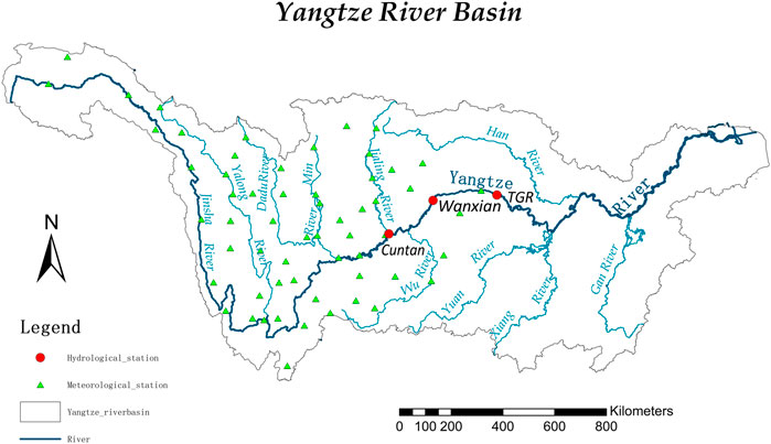
FIGURE 3. Research area and station distribution. Tan et al. (2018)

Model Inputs and Parameter Settings

When forecasting the daily inflows of the Three Gorges Reservoir, daily flows (inflows) measured for 1–7 days for the Three Gorges Reservoir and its upstream stations in Cuntan and Wanxian were selected as the predictors. Because runoff is a comprehensive result of meteorological and hydrological processes, the arithmetic average method was used to obtain the arithmetic average of the meteorological elements of the meteorological stations upstream of the Three Gorges Reservoir, and the meteorological elements from the previous 7 days to the forecast day were used as the model forecast factors. The meteorological elements considered by the model included rainfall, relative humidity, light, daily average temperature, and wind speed; thus, there were 5 + 8 × 7 forecast factors in the forecast factor set. LSTM uses a month of previous data as the input for each simulation. Both the inflow and predictor data series of the Three Gorges Reservoir use daily data from 2004 to 2017. The data from 2004 were used as preliminary predictors, and the data from 2005 to 2017 were used for model training and testing. The 2014 data were used as the training set, and the 2015–2017 data were used as the test set. The data were obtained from the Information Center of the Ministry of Water Resources.

In the EEMD model, the white noise amplitude was set to 0.2 times the standard deviation of the sample data, NR was set to 100, and the maximum number of filtering iterations was set to 500. Each decomposed sub-sequence must establish a unique LSTM model; thus, ${\displaystyle \sum _{\text{i}=1}^{12}\text{m}}\text{i}+M$ models must be established, where m_i is the number of series in the ith month, and M is the number of sub-series divided by the number of natural flow series.

In the LSTM model, the number of hidden layers was 1, the number of neurons in the hidden layer n was proportional to the complexity of the model, the value was 2^k (k = 1,2,3,...,10), and the sequence value range was [2,7]. For training, the learning rate was set to 0.0005, and the maximum training generation m was 500 generations. The model adopts the z-score algorithm for standardization. After standardization, the mean value of the data was 0, and the standard deviation was 1. In this study, the training and test sets were standardized Tan et al. (2018) separately, and the mean and standard deviation used in the calculation and de-standardization of the model results were derived from the training set.

Verification Strategy

To quantify the performance of the LSTM model, this study used three indicators, the Nash coefficient (NSE), relative deviation (BIAS), and mean absolute percentage error (MAPE), to evaluate the forecast accuracy of the model. The value range of the NSE was [−∞, 1]. The closer the value is to 1, the higher the degree of fit between the simulated and measured values. BIAS was used to evaluate the accuracy of the overall water balance of the model results, and the value range was [−100%, 100%]. The optimal value is 0; a positive value indicates that the water volume is higher overall. MAPE was used to reflect the relative deviation between the forecast and measured values; the value range was [0,100%], and the month was close to 0. The corresponding formulas are as follows:

$NSE=1-\frac{{\displaystyle \sum _{i=1}^N{\left(y_i-{\widehat{y}}_i\right)}^2}}{{\displaystyle \sum _{i=1}^N{\left(y_i-\overline{y}\right)}^2}}(15)$

$BIAS=\frac{{\displaystyle \sum _{i=1}^N\left({\widehat{y}}_i-y_i\right)}}{{\displaystyle \sum _{i=1}^N{y}_i}}\times 100\%(16)$

$MAPE=\frac{1}{N}{\displaystyle \sum _{i=1}^N\left|\frac{{\text{y}}_{\text{i}}-{\widehat{y}}_i}{y_i}\right|}\times 100\%(17)$

where i is the ith moment, N is the total number of time steps, represents the simulation value, y represents the observation value, and $\text{y}(-)$ is the mean value of the observation data.

Results and Discussion

Decomposition Results Using EEMD

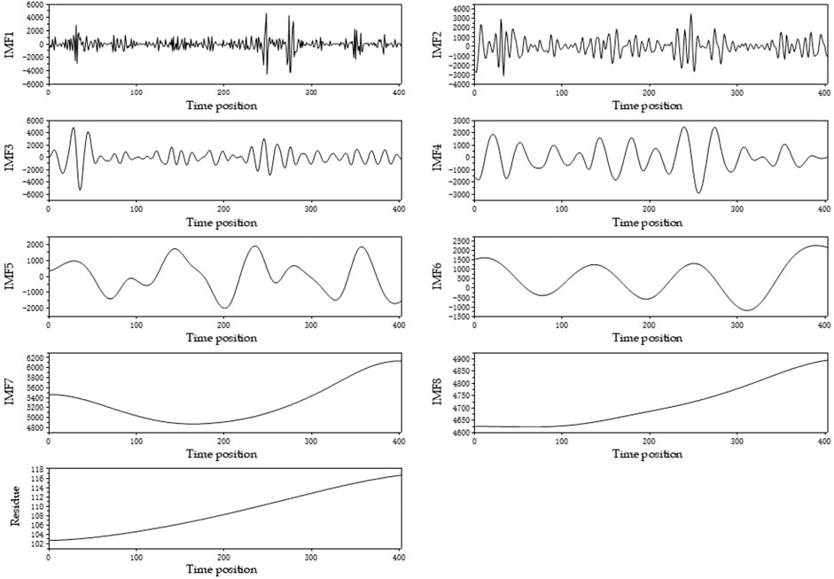
EEMD was used to decompose non-linear and non-stationary raw flow data into linear and stable sub-sequences. The monthly runoff sequence of the GM-EEMD-LSTM model was divided into eight or nine independent sub-sequences. In addition, the original sequences from 2005 to 2017 were broken down into 13 independent levels in the EEMD-LSTM model. The frequency of these components gradually decreased from IMF1 to IMFn, and the residual was the slowest trend of the original sequence. Due to space constraints, Figure 4 displays the decomposition results of the May month sequence of the GM-EEMD-LSTM model.

FIGURE 4

FIGURE 4. Components decomposed by EEMD for May.

Figure 4 displays the sub-sequences of different periods. IMF1 is short, with a higher frequency and greater fluctuation. The positions of IMF1, IMF2, and IMF3 related to larger amplitude fluctuations are consistent. IMF3 contains 13 cycles in total, which is consistent with the original sequence (2005–2017). The residue was the upward change trend of the data in May, which is consistent with the slight upward trend of the May monthly series.

Correlations Between Related Factors and Original/Decomposed Components

Through a cross-correlation analysis, the correlation coefficients between the forecast factors and flow series (LSTM, EEMD-LSTM, and GM-EEMD-LSTM model target series) were assessed, and the forecast factor with the largest mutual information value was selected as the model input.

The original sequence, the target sequence of the LSTM model, and the sub-sequences decomposed by EEMD based on the original sequence are counted and displayed in Table 1.

TABLE 1

TABLE 1. Top three maximum mutual information values of original and decomposed series.

Based on Table 1, the high-frequency sub-sequences exhibit a higher correlation with the runoff sequences of the Three Gorges Reservoir, while the lower-frequency sub-sequences are related to the runoff sequences of the Three Gorges Reservoir and Wanxian. Residual items and sub-items whose periods are close to trend items exhibit higher correlations with meteorological elements. The original data series exhibit the highest correlation with the runoff series of the previous day, and that of the mutual information is much higher than that of the highest mutual trust coefficient of each sub-sequence after EEMD decomposition.

This study also analyzed the mutual confidence coefficients between the sub-sequences of the GM-EEMD-LSTM model and the predictors after decomposing the monthly sequence. Figure 5 displays certain sub-sequences of the GM-EEMD-LSTM model (1, 5, and 9). Based on Figure 5A, the residue in January exhibited the strongest correlation with the traffic sequence of Wanxian, reaching its peak on day 3. IMF7 exhibited the strongest correlation with the flow of Wanxian on day 4, and it exhibited a strong correlation with meteorological elements compared with other sub-series except that of residue. Both IMF6 and IMF5 were strongly correlated with the runoff series of the Three Gorges Reservoir and Wanxian County, and the peak value was the runoff of Wanxian on day 6. IMF4 and IMF3 exhibited strong correlations with the runoff sequence of Cuntan and the Three Gorges Reservoir. IMF4 exhibited the strongest correlation with the Three Gorges Reservoir on day 1, and IMF3 had the strongest correlation with Cuntan on day 1. The other two graphs in Figure 5 display similar characteristics; sub-sequences with high frequencies are more likely to be highly correlated with Cuntan and the Three Gorges Reservoir, while sub-sequences with low frequencies are more likely to be correlated with Wanxian and the Three Gorges Reservoir. The trend item and IMFn are highly correlated with meteorological elements, which is consistent with the sub-sequences of the EEMD-LSTM model above.

FIGURE 5

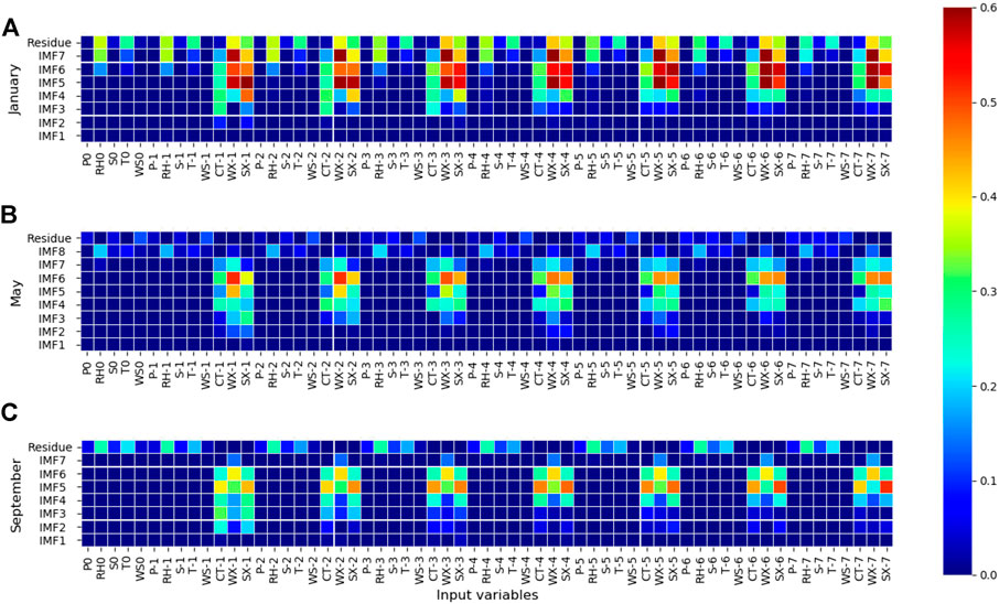
FIGURE 5. Two-dimensional correlations between model inputs and sub-inflow series by month. Vertical axis indicates the lag time, and the horizontal axis represents the indices. The redder the color, the greater the correlation. Sub-inflow series correspond to (A) January (B) May, and (C) September.

Optimal Parameters of LSTM Model for Decomposed Series

Statistical analysis was performed on the target sequence of the EEMD-LSTM model. Thirteen sub-sequences were decomposed by the EEMD of the original sequence, and statistical analysis was performed on the optimal parameters. IMF1 exhibited the highest frequency, and the optimal parameter values of the LSTM model were seq = 7, n = 128, and m = 100. The optimal parameter values of IMF12 and residue were seq = 3, n = 1,024, and m = 70.

The LSTM parameters were calculated when the prediction results of each sub-sequence of the 12-month sequence of the GM-EEMD-LSTM model were optimal, and a two-dimensional correlation diagram was obtained, as displayed in Figure 6. In the figure, IMF9 is the residue obtained by decomposing the sequence with the number of sub-sequences of 9, and the sequence residue with eight sub-sequences is IMF8 when IMF9 is blank.

FIGURE 6

FIGURE 6. Two-dimensional correlations between model parameters and sub-inflow series.

Based on Figure 6A, it can be seen that the sequence values of IMF7, IMF8, and IMF9 are proportionally smaller, while the period of IMF7–MF9 is long, which is substantially different from the input variable period. This result can be obtained by inputting less information during the simulation. The analysis illustrated in Figure 6B demonstrates that the ratio of IMF1–IMF4 to IMF7–IMF9, where the number of hidden neurons is less than n, is great. IMF7–IMF9 is more complicated because the period is significantly larger than that of the input variable. The proposed model can simulate this period more accurately than the simple model. Figure 6C demonstrates that IMF7–IMF9 is smaller than the other sub-sequence training times. Because the n value of IMF7–IMF9 is higher, the model is more complicated and has a stronger fitting ability; thus, when the number of training values is large, over-fitting can be easily caused. This is consistent with the sub-sequence parameter selection rule of the EEMD-LSTM model.

Model Performance Evaluation

Effectiveness Evaluation of EEMD Method

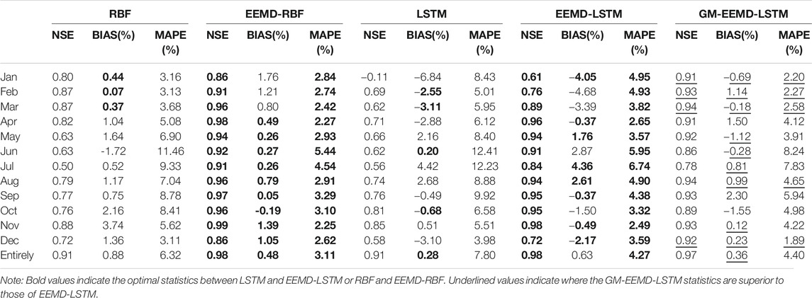
To evaluate the effectiveness of the EEMD method across multiple directions, this study uses the LSTM, EEMD-LSTM, and GM-EEMD-LSTM models to establish a model with a forecast period of 0 day to forecast the inflows of the Three Gorges Reservoir from 2015 to 2017. The predictor with the highest cross-correlation information for the measured runoff sequence was selected as the model input to predict the runoff sequence. The prediction ability of the different models was evaluated with NSE, BIAS, and MAPE. To study the simulation characteristics of the EEMD-LSTM model for different months of runoff, after evaluating the test set with the evaluation indicators, the prediction results of the test set were also counted on a monthly basis, whose results are listed in Table 2.

TABLE 2

TABLE 2. Model performances.

According to the analysis (Table 2), the simulation effect of the decomposition sequence was superior to that of the original series. In other words, the model performance of the EEMD-LSTM and EEMD-RBF models is better than the simulation performance of the LSTM and RBF models, especially for the NSE and MAPE indicators.

The LSTM model does not exhibit any clear rules for the runoff sequences of different months. A comparison between the EEMD-LSTM and GM-EEMD-LSTM models demonstrates that the GM-EEMD-LSTM model simulates the high-flow months (April to November) well. The result is slightly lower than that of the EEMD-LSTM model, but the overall performance in the low-water months (January, February, March, and December) was significantly better than that of the EEMD-LSTM model. Figure 7 displays the simulation results for January and May.

FIGURE 7

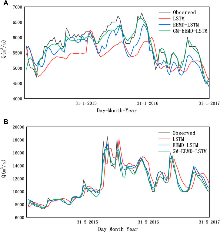
FIGURE 7. Comparison of forecast and original inflow values for 2015–2017 for the Three Gorges Reservoir.

Based on Figure 7, the decomposed model can more accurately simulate the peak and valley values of the runoff sequence. The GM-EEMD-LSTM simulation result was the closest to the measured value, while the results of the EEMD-LSTM model were the best in May. The results of both models were far superior to those of the undecomposed model. Therefore, the two methods can be combined to predict traffic. The EEMD-LSTM model can be used to make predictions in high-traffic months, and the GM-EEMD-LSTM model can be used to make predictions in low-flow months.

In addition, when the LSTM model is used alone for runoff prediction research, there is a widespread delay problem that manifests as translational misalignments on the images (Kratzert et al., 2018; Xiang et al., 2020). As displayed in Figure 7, the predicted values of the LSTM model vary and are slower to predict than the true value. This is because the LSTM network cannot accurately detect the degree of fluctuation in a time series; thus, the result of the prediction from the previous moment may be reflected at the present moment. The decomposition model using the EEMD method effectively remedies this issue. The time series is decomposed into several sub-sequences. Compared with the original series, the fluctuation degree of the sub-sequences is more stable, and it is easier to obtain the time-series fluctuations of each LSTM unit. The prediction of the network sub-model is more accurate, solving the delay problem of the LSTM network.

Results for Different Forecast Periods

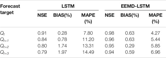
To evaluate the effect of EEMD on LSTM more comprehensively, this research established EEMD-LSTM and LSTM models for different forecast periods (0–3 day, represented as Q_t, Q_t+1, Q_t+2, and Q_t+3). And all forecast periods are based on falling rain. The results are displayed in Table 3.

TABLE 3

TABLE 3. Forecast results for different forecasting periods.

Based on Table 3, the EEMD-LSTM exhibits a superior forecasting performance. For all forecast periods, the BIAS indicators of the LSTM and EEMD-LSTM models are less than 5%, indicating that the LSTM model water balance is accurate. As the forecast period increases, the BIAS indicator value of the LSTM model significantly increases. However, the BIAS index of the EEMD-LSTM model is irregular, indicating that the EEMD method can improve the accuracy of the overall water balance of the model when the forecasting period increases. Both models exhibit the greatest effect when forecasting Q_t runoff. As the forecast period increased, the forecast accuracy decreased, and the forecast accuracy of the EEMD-LSTM model decreased less than that of the LSTM model. When the forecast period was 3 day, the Nash coefficients of the LSTM and EEMD-LSTM models were 0.79 and 0.94, respectively.

Conclusion

This study uses approximately 14 years of historical, meteorological, and runoff data as the forecast factor set and employs EEMD, mutual information, and LSTM for data processing, forecast factor selection, and runoff forecasting, respectively. The results demonstrate that the prediction performance of the LSTM model can be improved through EEMD processing. Based on the study results, the following conclusions can be drawn.

1 After the data was processed by EEMD, sub-sequences with different frequencies were obtained. The high-frequency sub-sequences exhibited a higher correlation with the runoff sequences of Cuntan and the Three Gorges Reservoir, while the lower-frequency sub-sequences were related to the runoff sequences of the Three Gorges Reservoir and Wanxian. The other items and sub-items with periods close to those of the trend items were highly correlated with meteorological elements. The original series exhibited the highest correlation with the data series of the day prior to the forecast, and the mutual information value was substantially higher than those of the sub-sequence and input variables. However, the decomposed series exhibited superior simulation results in the LSTM model.

2 The parameters of the LSTM model for sub-sequences with different frequencies presented the following laws: sub-sequences with low frequencies and longer periods contained less input information during simulation, more hidden neurons, were part of a more complex model, and exhibited higher training times. Additionally, the sequence parameter value was smaller, the n value was greater, and the m value was smaller.

3 The results demonstrate that the prediction results of the sub-series obtained by the LSTM and RBF exhibited better statistical performance than those of the original series.

4 The EEMD-LSTM model performs well across forecasting periods. As the forecast period increases, the forecasting accuracy decreases.

The combination of EEMD and LSTM methods for hydrological series prediction is the main novelty of this study. Moreover, while considering the autocorrelation in the runoff series, this study also considered its relationship with meteorological elements. In addition, when selecting the model input, the mutual information method suitable for linear and nonlinear relationships was selected. However, the correlation between the final model input and the prediction sequence was not strong enough, which will affect the model performance. Thus, further improvements are needed in regard to the correlation.

Data Availability Statement

The original contributions presented in the study are included in the article/Supplementary Material, further inquiries can be directed to the corresponding author.

Author Contributions

RY, WL, SC, and XL contributed to the design of the study and the discussion, and they wrote a draft of the manuscript. ZY, GD, JW, and YX organized the methodology. RY and YZ wrote individual sections of the manuscript. All authors contributed to manuscript revisions and have read and approved the submitted version.

Funding

This work was jointly supported by the National Key R&D Program of China (2017YFB0203104) and the National Natural Science Fund (51709273).

Conflict of Interest

Author ZY was employed by the company China Three Gorges Corporation.

The remaining authors declare that the research was conducted in the absence of any commercial or financial relationships that could be construed as a potential conflict of interest.

Acknowledgments

The authors are grateful to the information center at the Ministry of Water Resources of the People’s Republic of China for the provisioning of reservoir and hydrological data.

References

Abbaspour, K. C., Rouholahnejad, E., Vaghefi, S., Srinivasan, R., Yang, H., and Kløve, B. (2015). A continental-scale hydrology and water quality model for Europe: calibration and uncertainty of a high-resolution large-scale SWAT model. J. Hydrol. 524, 733–752. doi:10.1016/j.jhydrol.2015.03.027

CrossRef Full Text | Google Scholar

Adamowski, J., Morin, E., and Karran, D. J. (2014). Multi-step streamflow forecasting using data-driven non-linear methods in contrasting climate regimes. J. Hydroinformatics 16 (3), 671–689. doi:10.2166/hydro.2013.042

CrossRef Full Text | Google Scholar

Ahmadi, M., Moeini, A., Ahmadi, H., Motamedvaziri, B., and Zehtabiyan, G. R. (2019). Comparison of the performance of SWAT, IHACRES and artificial neural networks models in rainfall-runoff simulation (case study: Kan watershed, Iran). Phys. Chem. Earth, Parts A/B/C 111, 65–77. doi:10.1016/j.pce.2019.05.002

CrossRef Full Text | Google Scholar

An, L., Hao, Y., Yeh, T.-C. J., Liu, Y., Liu, W., and Zhang, B. (2020). Simulation of karst spring discharge using a combination of time-frequency analysis methods and long short-term memory neural networks. J. Hydrol. 589, 125320. doi:10.1016/j.jhydrol.2020.125320

CrossRef Full Text | Google Scholar

Cheng, C.-t., Niu, W.-j., Feng, Z.-k., Shen, J.-j., and Chau, K.-w. (2015). Daily reservoir runoff forecasting method using artificial neural network based on quantum-behaved particle swarm optimization. Water 7 (12), 4232–4246. doi:10.3390/w7084232

CrossRef Full Text | Google Scholar

Ding, G. B., Nong, Z. X., Wang, C., Song, P. B., and Lei, X. H. (2019). Long-term runoff forecasting model based on MI-PCA and BP neural network in shiyang River Basin. China Rural Water and Hydropower (10), 66–69. (in Chinese).

Google Scholar

Huang, N. E., Shen, Z., Long, S. R., Wu, M. C., Shih, H. H., Zheng, Q., et al. (1998). The empirical mode decomposition and the Hilbert spectrum for nonlinear and non-stationary time series analysis. Proc. R. Soc. Lond. A. 454, 903–995. doi:10.1098/rspa.1998.019310.1098/rspa.1998.0193

CrossRef Full Text | Google Scholar

Huang, N. E., and Wu, Z. (2008). A review on Hilbert-Huang transform: method and its applications to geophysical studies. Rev. Geophys. 46 (2). doi:10.1029/2007rg000228

CrossRef Full Text | Google Scholar

Jiang, T., Kundzewicz, Z. W., and Su, B. (2008). Changes in monthly precipitation and flood hazard in the Yangtze River Basin, China. Int. J. Climatol. 28 (11), 1471–1481. doi:10.1002/joc.1635

CrossRef Full Text | Google Scholar

Kan, G., Li, J., Zhang, X., Ding, L., He, X., Liang, K., et al. (2016). A new hybrid data-driven model for event-based rainfall-runoff simulation. Neural Comput. Applic 28 (9), 2519–2534. doi:10.1007/s00521-016-2200-4

CrossRef Full Text | Google Scholar

Kratzert, F., Klotz, D., Brenner, C., Schulz, K., and Herrnegger, M. (2018). Rainfall-runoff modelling using long short-term memory (LSTM) networks. Hydrol. Earth Syst. Sci. 22 (11), 6005–6022. doi:10.5194/hess-22-6005-2018

CrossRef Full Text | Google Scholar

Lee, D., Lee, G., Kim, S., and Jung, S. (2020). Future runoff analysis in the mekong River Basin under a climate change scenario using deep learning. Water 12 (6), 1556. doi:10.3390/w12061556

CrossRef Full Text | Google Scholar

Meshram, S. G., Singh, V. P., Kisi, O., Karimi, V., and Meshram, C. (2020). Application of artificial neural networks, support vector machine and multiple model-ANN to sediment yield prediction. Water Resour. Manage. 34 (15), 4561–4575. doi:10.1007/s11269-020-02672-8

CrossRef Full Text | Google Scholar

Nanda, T., Sahoo, B., Beria, H., and Chatterjee, C. (2016). A wavelet-based non-linear autoregressive with exogenous inputs (WNARX) dynamic neural network model for real-time flood forecasting using satellite-based rainfall products. J. Hydrol. 539, 57–73. doi:10.1016/j.jhydrol.2016.05.014

CrossRef Full Text | Google Scholar

News and Focus (2015). The three Gorges project. Engineering 1 (1), 011–013. doi:10.15302/j-eng-2015022

CrossRef Full Text | Google Scholar

Patil, A., and Ramsankaran, R. (2017). Improving streamflow simulations and forecasting performance of SWAT model by assimilating remotely sensed soil moisture observations. J. Hydrol. 555, 683–696. doi:10.1016/j.jhydrol.2017.10.058

CrossRef Full Text | Google Scholar

Sharma, A. (2000). Seasonal to interannual rainfall probabilistic forecasts for improved water supply management: Part 1 - a strategy for system predictor identification. J. Hydrol. 239 (1-4), 232–239. doi:10.1016/s0022-1694(00)00346-2

CrossRef Full Text | Google Scholar

She, L., and You, X.-y. (2019). A dynamic flow forecast model for urban drainage using the coupled artificial neural network. Water Resour. Manage. 33 (9), 3143–3153. doi:10.1007/s11269-019-02294-9

CrossRef Full Text | Google Scholar

Tan, Q.-F., Lei, X.-H., Wang, X., Wang, H., Wen, X., Ji, Y., et al. (2018). An adaptive middle and long-term runoff forecast model using EEMD-ANN hybrid approach. J. Hydrol. 567, 767–780. doi:10.1016/j.jhydrol.2018.01.015

CrossRef Full Text | Google Scholar

Tayyab, M., Ahmad, I., Sun, N., Zhou, J., and Dong, X. (2018). Application of integrated artificial neural networks based on decomposition methods to predict streamflow at upper indus basin, Pakistan. Atmosphere 9 (12), 494. doi:10.3390/atmos9120494

CrossRef Full Text | Google Scholar

Tian, M., Zhou, J., Jia, B., Lou, S., and Wu, H. (2020). Impact of three Gorges reservoir water impoundment on vegetation-climate response relationship. Remote Sensing 12 (17), 2860. doi:10.3390/rs12172860

CrossRef Full Text | Google Scholar

Wang, J., Wang, X., Lei, X. h., Wang, H., Zhang, X. h., You, J. j., et al. (2020). Teleconnection analysis of monthly streamflow using ensemble empirical mode decomposition. J. Hydrol. 582, 124411. doi:10.1016/j.jhydrol.2019.124411

CrossRef Full Text | Google Scholar

Wang, W. C., Chau, K. W., Qiu, L., and Chen, Y. B. (2015). Improving forecasting accuracy of medium and long-term runoff using artificial neural network based on EEMD decomposition. Environ. Res. 139, 46–54. doi:10.1016/j.envres.2015.02.002

PubMed Abstract | CrossRef Full Text | Google Scholar

Wang, Z.-Y., Qiu, J., and Li, F.-F. (2018). Hybrid models combining EMD/EEMD and ARIMA for long-term streamflow forecasting. Water 10 (7), 853. doi:10.3390/w10070853

CrossRef Full Text | Google Scholar

Wu, J. S., Han, J., Annambhotla, S., and Bryant, S. (2005). Artificial neural networks for forecasting watershed runoff and stream flows. J. Hydrol. Eng. 10 (3), 216–222. doi:10.1061/(asce)1084-069910.1061/(asce)1084-0699(2005)10:3(216)

CrossRef Full Text | Google Scholar

Xiang, Z., Yan, J., and Demir, I. (2020). A rainfall‐runoff model with LSTM‐based sequence‐to‐sequence learning. Water Resour. Res. 56 (1). doi:10.1029/2019wr025326

CrossRef Full Text | Google Scholar

Yin, Z.-K., Liao, W.-H., Wang, R.-J., and Lei, X.-H. (2019). Rainfall-runoff modelling and forcasting based on long short-term memory(LSTM). South-to-North Water Transfers Water Sci. Tech. 17 (6). doi:10.13476/j.cnki.nsbdqk.2019.0129 (in Chinese).

CrossRef Full Text | Google Scholar

Yu, Y., Zhao, W., Martinez-Murillo, J. F., and Pereira, P. (2020). Loess Plateau: from degradation to restoration. Sci. Total Environ. 738, 140206. doi:10.1016/j.scitotenv.2020.140206

PubMed Abstract | CrossRef Full Text | Google Scholar

Yu, Y., Zhang, H., and Singh, V. (2018). Forward prediction of runoff data in data-scarce basins with an improved ensemble empirical mode decomposition (EEMD) model. Water 10 (4), 388. doi:10.3390/w10040388

CrossRef Full Text | Google Scholar

Zhang, X., Zhang, Q., Zhang, G., Nie, Z., Gui, Z., Que, H. F., et al. (2018). A novel hybrid data-driven model for daily land surface temperature forecasting using long short-term memory neural network based on ensemble empirical mode decomposition. Ijerph 15 (5), 1032. doi:10.3390/ijerph15051032

CrossRef Full Text | Google Scholar

Zhao, Steel., and Yang, D.-W. (2011). Mutual information-based input variable selection method for runoff -forecasting neural network model. J. Hydroelectric Eng. 30 (1), 24–30. (in Chinese).

Google Scholar

Zhao, X., Chen, X., Xu, Y., Xi, D., Zhang, Y., and Zheng, X. (2017). An EMD-based chaotic Least Squares support vector machine hybrid model for annual runoff forecasting. Water 9 (3), 153. doi:10.3390/w9030153

CrossRef Full Text | Google Scholar

Zhao, Y., Li, Z., Cai, S., and Wang, H. (2020). Characteristics of extreme precipitation and runoff in the Xijiang River Basin at global warming of 1.5 °C and 2 °C. Nat. Hazards 101 (3), 669–688. doi:10.1007/s11069-020-03889-x

CrossRef Full Text | Google Scholar

Zhou, J., Jia, B., Chen, X., Qin, H., He, Z., and Liu, G. (2019). Identifying efficient operating rules for hydropower reservoirs using system dynamics approach-A case study of three Gorges reservoir, China. Water 11 (12), 2448. doi:10.3390/w11122448

CrossRef Full Text | Google Scholar

Zhu, Q., Gao, X., Xu, Y.-P., and Tian, Y. (2019). Merging multi-source precipitation products or merging their simulated hydrological flows to improve streamflow simulation. Hydrological Sci. J. 64 (8), 910–920. doi:10.1080/02626667.2019.1612522

CrossRef Full Text | Google Scholar