 Jianlong Feng
 Huan Li1
95% of researchers rate our articles as excellent or good
Learn more about the work of our research integrity team to safeguard the quality of each article we publish.
Find out more
ORIGINAL RESEARCH article
Front. Earth Sci. , 27 November 2018
Sec. Atmospheric Science
Volume 6 - 2018 | https://doi.org/10.3389/feart.2018.00216
This article is part of the Research Topic Modelling, Simulating and Forecasting Regional Climate and Weather View all 12 articles
Using hourly sea level data from 15 tide gauges along the Chinese coast and sea level data of three simulations of the Coupled Model Intercomparison Project Phase 5 (CMIP5), we assessed the changes and benefits of the extreme sea level of limiting warming to 1.5∘C instead of 2.0∘C. Observations show that the extreme sea level has risen with high confidence during the past decades along the coast of China, while the mean sea level change, especially the long-term change plays important roles in the changing process of extreme sea levels. Under the 1.5 and 2.0∘C warming scenarios, the sea level will rise with fluctuations in the future, so will the return levels of the extreme sea levels. Compared with the 1.5∘C warming condition, the return levels under the 2.0∘C warming condition will rise significantly at all tide gauges along the Chinese coast. The results indicate that a 0.5∘C warming will bring much difference to the extreme sea levels along the coast of China. It is of great necessity to limit anthropogenic warming to 1.5∘C rather than 2.0∘C, as proposed by the Paris Climate Agreement, which will greatly reduce the potential risks of future flood disasters along the coast of China and is beneficial for risk response management.
China has the largest coastal population in the world, with more than 40% people living in the coastal area, where the extreme sea level disasters occur frequently and have caused serious negative impacts. According to the China Marine Disaster Bulletin1, the extreme sea level incidents have caused economic losses of 11.1 billion (RMB) and 49 deaths annually between 2000 and 2017.
Increases in the mean and extreme sea levels are regarded as one of the consequences of climate change (Church et al., 2013). In recent years, many studies have been done about the changes of extreme sea levels both regionally and globally (von Storch and Reichardt, 1997; Woodworth and Blackman, 2004; Méndez et al., 2007; Menéndez and Woodworth, 2010; Feng et al., 2015; Marcos and Woodworth, 2017). Substantial evidences have revealed the general increase in extreme sea level in the past decades worldwide. Many researches indicated that the changes of the extreme sea level, especially the long-term change, are highly correlated with the changes of mean sea level (Zhang et al., 2000; Woodworth and Blackman, 2004; Marcos et al., 2009; Menéndez and Woodworth, 2010; Tsimplis and Shaw, 2010). Meanwhile, statistical method and dynamical method are utilized to study the future changes in extreme sea level. The extreme sea levels will increase as mean sea levels rise in the future according to the future projection (Langenberg et al., 1999; Busuioc et al., 2006; Woth et al., 2006; Grossmann et al., 2007).
Compared with the mean sea level (Ding et al., 2001; Yu et al., 2003; Zuo et al., 2007; Wang et al., 2018), fewer studies have been conducted to analyze the extreme sea levels along the China coast in the past. Chen and Wang (1993) found that the extreme sea level at Wusong and Huangpu Park increased between 1915 and 1985. Feng and Tsimplis (2014) and Feng et al. (2015) analyzed the changes of extreme sea levels using tide gauge data and indicated that the extreme sea level increased in the past decades, while the long-term change of extreme sea level was mainly affected by the change of mean sea level. Ma et al. (2016) discovered that the return levels of extreme sea level during 1980–2012 were higher than those during 1950–1979 at Tianjin. Due to the uneven distribution of tide gauges and data limitation, most studies above concentrated on the Yellow Sea, East China Sea, and the South China Sea. Besides, few work focuses on analyzing the future changes of extreme sea levels along the China coast.
The Paris Climate Agreement aims to hold global warming well below 2.0°C and to pursue efforts to limit it to 1.5°C above preindustrial temperature. Recently, increasing studies have been performed to investigate the extreme climate events at the 1.5 and 2°C warming levels and the superiority of limiting warming to 1.5°C rather than 2.0°C (Schleussner et al., 2016; Donnelly et al., 2017; Karmalkar and Bradley, 2017; King and Karoly, 2017; King et al., 2017; Lehner et al., 2017; Xu et al., 2017; Li et al., 2018). It is necessary to quantify the extreme sea levels changes under the 1.5 and 2.0°C warming scenarios and evaluate the differences between them.
In this paper, hourly sea level data from 15 tide gauges along the China coast and sea level data from three simulations of the Coupled Model Intercomparison Project Phase 5 (CMIP5) were used to answer the following questions: (1) How did the extreme sea level change during the past decades? (2) How will the extreme sea level change in future 1.5 and 2.0°C warming scenarios? (3) What will the extreme sea level differences be between 1.5 and 2.0°C warming climate?
Observed and numerical sea level data are applied in this study, including hourly sea level data from 15 tide gauges (Huludao, Qinhuangdao, Longkou, Yantai, Rizhao, Lusi, Dajishan, Zhenhai, Kanmen, Shansha, Xiamen, Shanwei, Zhapo, Haikou, and Beihai) along the China coast, and three CMIP5 simulations results downloaded from the online CMIP5 datasets (CNRM-CM5, BCC-CSMI-1, MIROC-ESM-CHEM).
The gauge data were obtained from the marine monitoring stations in China (Figure 1), dating from January, 1980 to December, 2016. All these data last for more than 30 years, which is essential to get the trends accurately (Feng et al., 2015). Careful quality control had been done to delete the data spikes and spurious records (Wang et al., 2013). In addition, data availability less than 60% were excluded in the analysis.
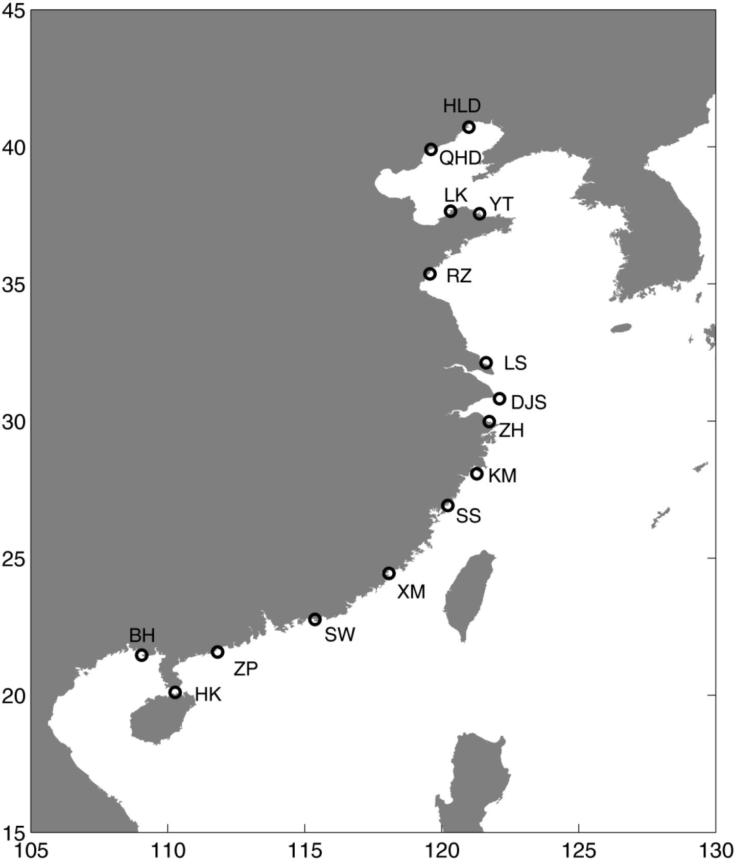
FIGURE 1. Locations of 15 tide gauges along the coast of China used in this work: HLD, Huludao; QHD, Qinhuangdao; LK, Longkou; YT, Yantai; RZ, Rizhao; LS, Lusi; DJS, Dajishan; ZH, Zhenhai; KM, Kanmen; SS, Shansha; XM, Xiamen; SW, Shanwei; ZP, Zhapo; HK, Haikou; and BH, Beihai.
The sea-level projection in this study is based on CMIP5 numerical simulations. Three models were selected in this work (Table 1). The sea level data reached the warming limits of 1.5 and 2.0°C were used. Two oceanic data categories, i.e., “zostoga” (the global average sea-level change due to thermal expansion) and “zos” (the local steric and dynamic adjustment of sea-level change) are used to project the regional sea level change. The data were modified in each model through the following procedures: (I) perform a quadratic-fit as a function of time at each grid point of the piControl experiment; (II) remove the quadratic-fitted control drift from the corresponding grid point of the historical and RCPs (Representative Concentration Pathways) experiments; (III) subtract the global mean of the “zostoga” and “zos” field at each time step from each grid point (Slangen et al., 2014). The projected contributions from land ice and land water storage to local sea-level change are obtained by multiplying the global mean estimates from IPCC AR5 by the regional scaling factors given by Slangen et al. (2014). All glaciers, ice caps and the ice sheets on Greenland and Antarctica are comprised in the land ice contribution. In addition, the glacier isostatic adjustment (GIA) is also included here (Slangen et al., 2014).
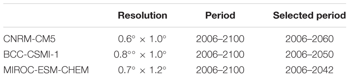
TABLE 1. The selected CMIP5 simulations.
Sea level data from tide gauge and satellite located in the Xisha (111.51°N, 16.44°E) were used to validate the sea level data from three models (Figure 2). Results show that although there are some differences between the observations and the model results at the interannual and decadal time scales, all three models are in good agreement with the observations at the long-term time scale. These results enhance the confidence in the quality of the projected data got from the three climate models.
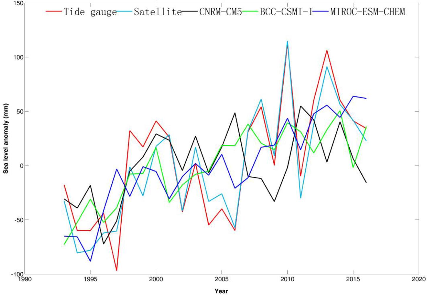
FIGURE 2. The sea level anomaly calculated using the data from the tide gauge, the satellite, CNRM-CM5, BCC-CSMI-l, and MIROC-ESM-CHEM during 1993 and 2016.
The extreme sea levels defined as the maximum level during a selected period, usually a year, were mainly caused by the storm surges. It was usually the maximum water level during a storm surge event. To calculate the precise extreme sea level rise rates and to identify potential rate changes are of vital importance for this study. In general, the sea level change trend is estimated by analyzing its oscillatory behavior, which means extracting periodic components from original observations successively until there is no periodic component left (Jevrejeva et al., 2006; Ezer and Corlett, 2012; Breaker and Ruzmaikin, 2013). Due to the empirical, intuitive, direct and adaptive characteristics, the empirical mode decomposition (EMD) method is suitable for estimating the accurate long-term trend of the sea level data (Huang et al., 1998, 1999) and has been widely used to get the long-term change of the mean sea levels recently (Ezer and Corlett, 2012; Breaker and Ruzmaikin, 2013; Ezer et al., 2013; Uranchimeg et al., 2013).
The EMD method decomposes an arbitrary time series X(t) into a finite and often small number of intrinsic mode functions (IMFs), which are defined as any function with an equal number of extreme and zero-crossing. Then X(t) can be described as:
where n is the number of IMFs, and rn is the residual. For more descriptions of the EMD method, refer to Huang et al. (1998).
Ensemble empirical mode decomposition (EEMD) is the improved method to obtain IMFs with more direct physical meaning and greater uniqueness (Wu and Huang, 2009). EEMD was estimated by averaging numerous EMD runs with the addition of some white noise. By averaging the different decompositions, the noise was averaged out and the true decomposition was calculated with a confidence estimate. The EEMD method was used to analyze the extreme sea levels in the study.
The risks associated with extreme sea levels can be assessed from the estimates of return levels and return periods. The return period of extreme sea level is defined as the sea level statistically expected to be equaled or exceeded every specific year. The Federal Emergency Management Agency [FEMA] (2004) recommended the frequency analysis metho3d to obtain the return levels. The traditional probability distribution methods, including the Gumbel, Weibull, Generalized Pareto Distribution (GPD), and Generalized Extreme Value (GEV) distributions, are typically used to analyze annual extreme sea levels. According to previous studies (Vogel et al., 1993; Huang et al., 2008; Feng and Jiang, 2015) the GEV distribution was used in this work to get the return levels of the extreme sea levels. As described in FEMA’S guideline (2014) the GEV distribution can be described by the probability density function (PDF) listed as follows:
for −∞ < x ≤ a − with c < 0
and a − ≤ x < ∞ with c > 0
for −∞ ≤ x < ∞ with c = 0
where, a, b, and c are the location, scale and shape factors.
Percentile analysis method has been widely used to assess the extreme sea level changes (Menéndez and Woodworth, 2010; Feng et al., 2015; Marcos and Woodworth, 2017). 99.9, 99, and 90% levels of the observed sea level have been calculated at all 15 tide gauges (Figure 3). Results show that the three percentile levels of extreme sea level all rose with fluctuations at nearly all tide gauges except at QHD, SW, and BH. Also the long-term trend was not significant at the 95% confidence level at QHD, LK, SW, KM, and BH. Results also show that the increase rates are different at different percentile levels. Meanwhile clear decadal variations and interannual variations exist in the extreme sea levels at all tide gauges. Especially the interannual variation was quite large at KM, SS, XM, and BH, where the amplitude of interannual variations were larger than 0.40 m.
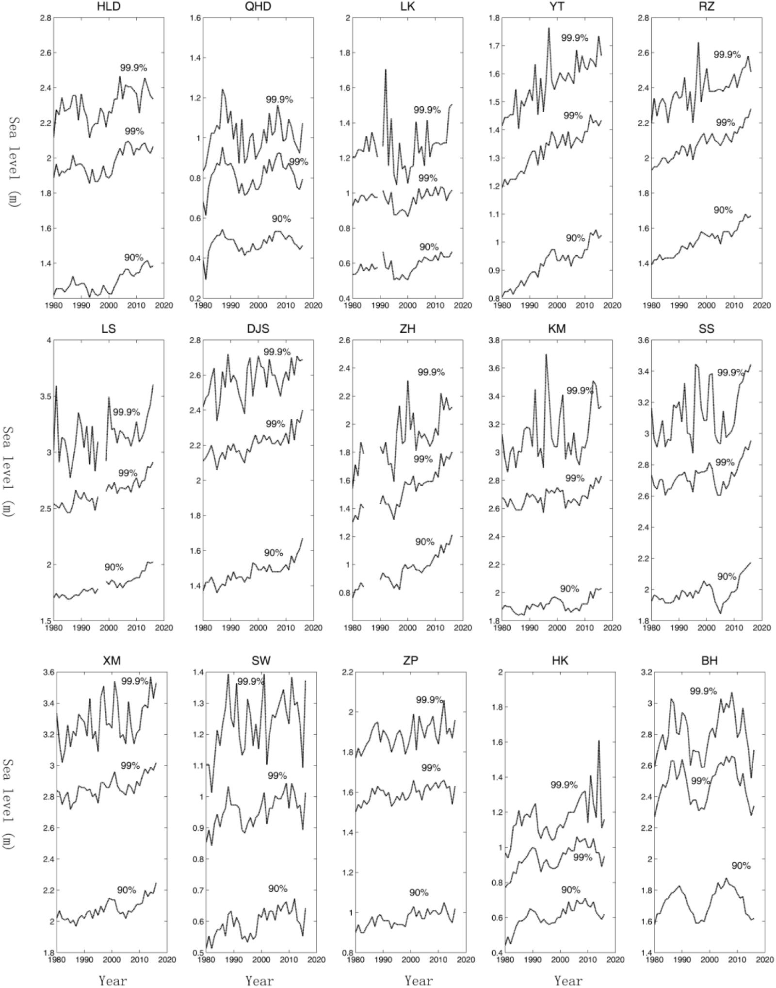
FIGURE 3. 99.9, 99, and 90% values of the observed sea level at 15 tide gauges.
Previous researches Feng and Tsimplis (2014) and Feng et al. (2015) show that the changes of extreme sea levels along the China coast were highly affected by the sea level change especially the long-term change. The correlations between the extreme sea level and mean sea level were calculated and shown in Table 2. Results show that the extreme sea levels were significantly correlated with the mean sea levels at most of the 15 tide gauges. The correlations were larger than 0.5 at YT, RZ, DJS, ZH, and SW. There are two tide gauges, LK and BH, where the extreme sea level was not significantly correlated with the mean sea level. Moreover, the correlation coefficients after detrending were also calculated. Results show that the correlations decrease after detrending. The correlation became non-significant at 95% significant level after detrending at HLD, YT, RZ, LS, XM, SW, ZP, and HK. Results indicate that the changes of mean sea level play important roles in the changes of extreme sea level along the China coast, and mean sea levels mainly affected the long-term change of the extreme sea levels. This conclusion coincides with previous studies, which indicated that the long-term trend of the extreme sea levels was mainly affected by the mean sea levels (Zhang et al., 2000; Woodworth and Blackman, 2004; Marcos et al., 2009).
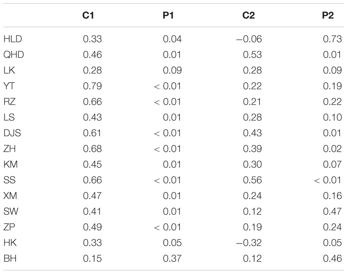
TABLE 2. Correlation coefficient between the extreme sea level and mean sea level at 15 tide gauges (C1) and the correlations after detrending (C2), the P1/P2 are the p-value from t-test (where p < 0.05 means that the correlation was significant at 95% confidence level).
Using the EEMD method the long term trends of the extreme sea levels along the Chinese coast were estimated in the study. Figure 4 shows that the extreme sea levels along the Chinese coast show increase trend in general. Meanwhile the long term trends show various patterns at different tide gauges. At HLD, LK, KM, and BH the increase rate accelerates during the past years. At YT, RZ, DJS, ZH, XM, and SS the increase trends were nearly linear. At QHD, SW, and ZP the increase trends were not significant at 95% confidence level. At LS the increase rate first slowed down but after 2000 the increase rate accelerated. At HK the increase trend slowed down during the past years.
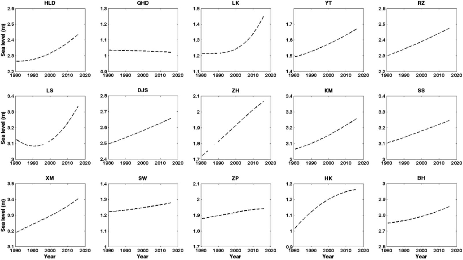
FIGURE 4. Long term trends of the extreme sea levels at 15 tide gauges along the Chinese coast.
The projected sea levels from three simulations of the CMIP5 were used in the work (section Data). The sea level data reached the 1.5 and 2.0°C scenario of three models were shown in Figure 5. Results show that the sea level of the three selected models rise with fluctuations. The sea levels were much higher at the 2.0°C warming conditions than the 1.5°C warming conditions at all three models. Among the three models the sea level of the MIROC-ESM-CHEM increased the fastest. The increase rate of the CNRM-CM5 and BCC-CSMI-1 is nearly the same. The CNRM-CM5 reached 1.5°C warming conditions in 2038 and reached 2.0°C warming conditions in 2060. The BCC-CSMI-1 and MIROC-ESM-CHEM reached 1.5 and 2.0°C warming conditions earlier than the CNRM-CM5.
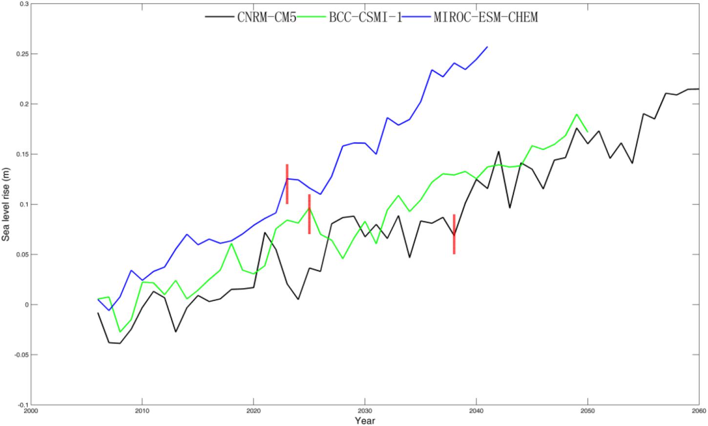
FIGURE 5. The sea level rise (compared with the mean sea level from 1985 to 2016) of three models under RCP4.5 scenarios, the sea level rise reached the 2°C scenario (whole line), the sea level rise reached the 1.5°C scenario (2006- red line break).
Using the method described in section Methodology the return levels of the extreme sea level under the 1.5 and 2.0°C warming conditions were calculated. Figures 6, 7 show that the return levels of the extreme sea level changed under the 1.5 and 2.0°C warming conditions. And the differences between the 1.5 and 2.0°C scenarios were quite large. Under the 1.5°C warming condition the changes of the return levels were small. At some tide gauges there are nearly no changes in the return levels. Under 2.0°C warming condition the return levels of the extreme sea level of three models significant increased. In order to show the changes of the return levels more clearly, the 100-year return levels under three scenarios were calculated and shown in Table 3.
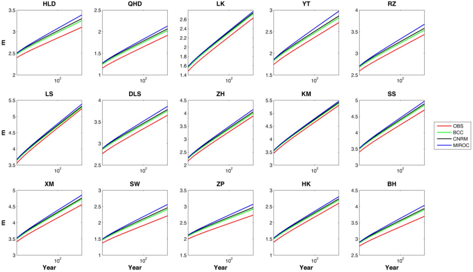
FIGURE 6. Return levels of the extreme sea level at present (blue line), return levels of the extreme sea level under the 1.5°C temperature rise scenarios [BCC-CSMI-1(black line), CNRM-CM5(red line), MIROC-ESM-CHEM(green line)].
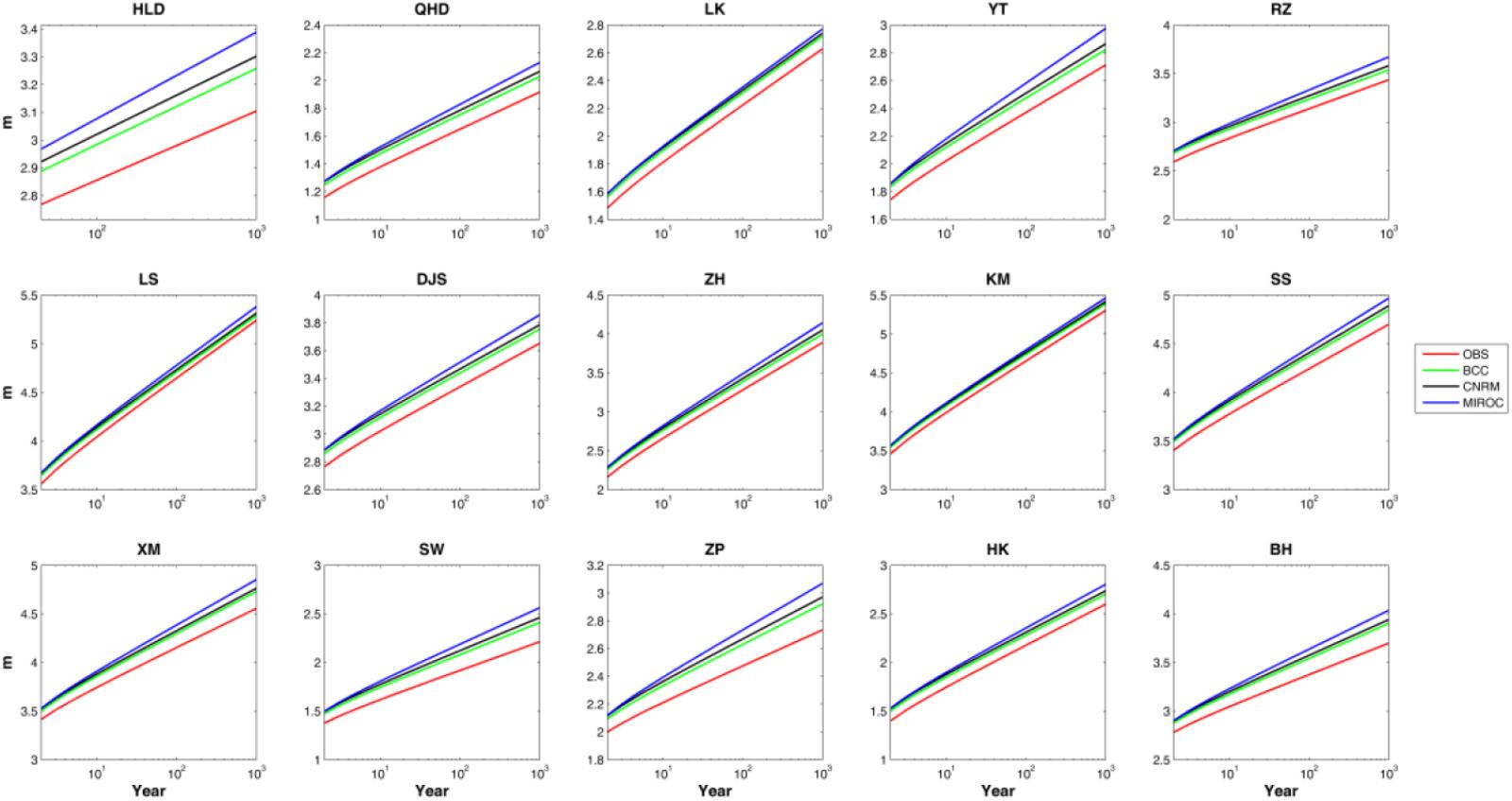
FIGURE 7. Return levels of the extreme sea level at present (blue line), return levels of the extreme sea level under the 2.0°C temperature rise scenarios [BCC-CSMI-1(black line), CNRM-CM5(red line), MIROC-ESM-CHEM(green line)].
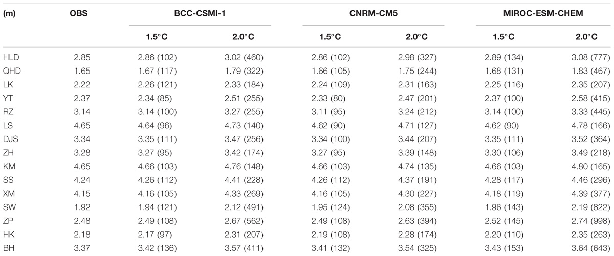
TABLE 3. Hundred-year return levels of the extreme sea level in present (unit is meter), under the 1.5 and 2°C scenario (from climate model) at 15 tide gauges, the return period (year) of the water levels in present scenario were listed in the bracket.
Compared with the present scenario, the 100-year return levels under the 1.5°C warming condition changed little at most tide gauges in BCC-CSMI-1 and CNRM-CM5. The 100-year return level changes ranged from -3 to 5 cm in BCC-CSMI-1. And in CRRM-CM5 the 100-year return level changes ranged from -4 to 4 cm. The changes of 100-year return levels in MIROC-ESM-CHEM ranged from -3 to 6 cm, and the 100-year return levels were larger than in the other two models at most tide gauges.
Under the 2.0°C warming condition, the changes of 100 year return levels were much larger than those under the 1.5°C warming condition in all three models. In BCC-CSMI-1 the 100-return level changes ranged from 8 to 20 cm, and the 100-year return levels correspond to the water levels of 140∼562 year return period under the present condition. Comparing to the 1.5°C warming condition the 100-year return levels increased about 4∼18 cm. In CNRM-CM5 the 100-return level changes ranged from 6 to 17 cm, and the 100 year return levels under the 2.0°C warming condition correspond to the water levels of 127∼394 return period under the present condition. Comparing to the 1.5°C warming condition the 100 year return levels increased about 8∼14 cm. In MIROC-ESM-CHEM the 100 return level changes ranged from 13 to 27 cm, and the 100 year return levels under the 2.0°C warming condition correspond to the water levels of 165∼998 year return period under the present condition. Comparing to the 1.5°C warming condition the 100-year return levels increased about 10∼23 cm. Results indicated that a 0.5°C warming will make much difference in the extreme sea levels along the Chinese coast in all three models.
The growing concerns about climate change have motivated numerous researchers to study the effects of climate change in coastal areas. As one of the most important marine factors in coastal areas, extreme sea level has drawn more and more attentions in recent years. In this paper, we used hourly sea level data from 15 tide gauges along the China coast and numerical sea level data from three simulations of the CMIP5, to analyze the changes of extreme sea level in the past and under the 1.5 and 2°C warmer future scenarios.
The extreme sea levels rise with fluctuations at most tide gauges along the China coast, and the long term trends show various patterns. Quasi-linear trends are found at YT, RZ, DJS, ZH, XM, and SS, while no significant trends exists at QHD, SW, and ZP. The extreme sea level starts to rise since 2000 at LS, and the rise decelerates at HK during the past years. The mean sea level changes play important roles in the changes of extreme sea levels along the China coast, especially for the long-term change.
Under the 1.5 and 2.0°C warming scenarios, the sea level rise with fluctuations according to the simulation results by three selected models, and the sea levels are much higher under the 2.0°C warming scenarios. The return levels of the extreme sea level vary significantly under different warming scenarios, and there is considerable increase of the return levels at all tide gauges along the China coast under 2.0°C warming scenario compared with that under 1.5°C warming scenario. The results indicated that a 0.5°C warming will bring about major difference for the extreme sea levels along the China coast. It is reasonable to limit the anthropogenic warming to 1.5°C rather than 2.0°C based on this study, as proposed by the Paris Climate Agreement, and it is necessary and practical for future flood risk management and response along the coast of China.
There are also some caveats in this study. In order to meet the warming condition of 1.5 and 2.0°C, the data lengths of the three model here are different. And only three models are analyzed in this study and there may be some uncertainty in the results presented in this manuscript. Besides, only the results of the RCP4.5 scenario were applied in this work.
JF conceptualized the research and contributed to the discussion and interpretation of the results. HL gave the sea level rise results used in this work. DL, QL, HW, and KL prepared and conducted some of the data analysis in the work. All authors contributed to the revision and approved the manuscript.
This work was supported by the National Key Research Projects (Grant Nos. 2016YFC1401900, 2017YFC1404200, 2017YFA0604101, and 2017YFA0604102), and the National Natural Science Foundation of China (Grant Nos. 41706020 and 41406032) and Open Fund if the Key Laboratory of Research on Marine Hazards Forecasting and the National Natural Science Foundation of China (41706019).
The authors declare that the research was conducted in the absence of any commercial or financial relationships that could be construed as a potential conflict of interest.
Breaker, L. C., and Ruzmaikin, A. (2013). Estimating rates of acceleration based on the 157-year record of sea level from San Francisco, California, U.S.A. J. Coast. Res. 29, 43–51. doi: 10.2112/JCOASTRES-D-12-00048.1
Busuioc, A., Giorgi, F., Bi, X., and Ionita, M. (2006). Comparison of regional climate model and statistical downscaling simulations of different winter precipitation change scenarios over Romania. Theor. Appl. Climatol. 86,101–123. doi: 10.1007/s00704-005-0210-8
Chen, S., and Wang, B. (1993). Analysis of maximum water level in the Changjiang estuary. J. East China Norm. Univ. 3, 75–82.
Church, J., Clark, P., Cazenave, A., Gregory, J., Jevrejeva, S., Levermann, A., et al. (2013). “Sea level change,” in Climate Change 2013: The Physical Science Basis. Contribution of Working Group in the Fifth Assessment Report of the Intergovernmental Panel on Climate Change, eds T. F. Stocker, D. Qin, G.-K. Plattner, M. Tignor, S. K. Allen, J. Boschung, et al. (Cambridge: Cambridge University Press).
Ding, X., Zheng, D., Chen, Y., Chao, J., and Li, Z. (2001). Sea level change in Hong Kong from tide gauge measurements of 1954-1999. J. Geod. 74, 683–689. doi: 10.1007/s001900000128
Donnelly, C., Greuell, W., Andersson, J., Gerten, D., Pisacane, G., Roudier, P., et al. (2017). Impacts of climate change on European hydrology at 1.5, 2 and 3 degrees mean global warming above preindustrial level. Clim. Change 143, 13–26. doi: 10.1007/s10584-017-1971-7
Ezer, T., Atkinson, L. P., Corlett, W. B., and Blanco, J. L. (2013). Gulf Stream’s induced sea level rise and variability along the U.S. mid-Atlantic coast. J. Geophys. Res. 118, 685–697. doi: 10.1002/jgrc.20091
Ezer, T., and Corlett, W. B. (2012). Is sea level rise accelerating in the Chesaperake Bay? A demonstration of a novel new approach for analyzing sea level data. Geophys. Res. Lett. 39:L19605.
Federal Emergency Management Agency [FEMA] (2004). Final Draft Guidelines for Coastal Flood Hazard Analysis and Mapping for the Pacific Coast of the United States. Washington, DC: FEMA.
Feng, J., and Jiang, W. (2015). Extreme water level analysis at three stations on the coast of the Northwestern Pacific Ocean. Ocean Dyn. 65, 1383–1397. doi: 10.1007/s10236-015-0881-3
Feng, J., von Storch, H., Jiang, W., and Weisse, R. (2015). Assessing changes in extreme sea levels along the coast of China. J. Geophys. Res. Ocean 120, 8039–8051. doi: 10.1002/2015JC011336
Feng, X., and Tsimplis, M. N. (2014). Sea level extremes at the coasts of China. J. Geophys. Res. Ocean 119, 1593–1608. doi: 10.1002/2013JC009607
Grossmann, I., Woth, K., and von Storch, H. (2007). Localization of global climate change: storm surge scenarios for Hamburg in 2030 and 2085. Die Küste 71, 169–182.
Huang, N. E., Shen, Z., and Long, S. R. (1999). A new view of nonlinear water waves: the Hilbert spectrum. Annu. Rev. Fluid Mech. 31, 417–457. doi: 10.1146/annurev.fluid.31.1.417
Huang, N. E., Shen, Z., Long, S. R., Wu, M. C., Shih, E. H., Zheng, Q., et al. (1998). The empirical mode decomposition and the Hilbert spectrum for non stationary time series analysis. Proc. R. Soc. Lond. 454, 903–995. doi: 10.1098/rspa.1998.0193
Huang, W., Xu, S., and Nnaji, S. (2008). Evaluation of GEV model for frequency analysis of annual maximum water levels in the coast of United States. Ocean Eng. 35, 1132–1147. doi: 10.1016/j.oceaneng.2008.04.010
Jevrejeva, S., Grinsted, A., Moore, J. C., and Holgate, S. (2006). Nonlinear trends and multiyear cycles in sea level records. J. Geophys. Res. 11:C09012. doi: 10.1029/2005JC003229
Karmalkar, A. V., and Bradley, R. S. (2017). Consequences of global warming of 1.5°C and 2°C for regional temperature and precipitation changes in the contiguous United States. PLoS One 12:e0168697. doi: 10.1371/journal.pone.0168697
King, A. D., and Karoly, D. J. (2017). Climate extremes in Europe at 1.5 and 2 degrees of global warming. Environ. Res. Lett. 12:114031. doi: 10.1088/1748-9326/aa8e2c
King, A. D., Karoly, D. J., and Henley, B. J. (2017). Australian climate extremes at 1.5°C and 2°C of global warming. Nat. Clim. Change 7, 412–416. doi: 10.1038/nclimate3296
Langenberg, H., Pfi zenmayer, A., von Storch, H., and Sündermann, J. (1999). Storm related sea level variations along the North Sea coast: natural variability and anthropogenic change. Cont. Shelf Res. 19, 821–842. doi: 10.1016/S0278-4343(98)00113-7
Lehner, F., Coats, S., Stocker, T. F., Pendergrass, A. G., Sanderson, B. M., Raible, C. C., et al. (2017). Projected drought risk in 1.5°C and 2°C warmer climates. Geophys. Res. Lett. 44, 7419–7428. doi: 10.1002/2017GL074117
Li, D., Zhou, T., Zou, L., Zhang, W., and Zhang, L. (2018). Extreme high temperature events over East Asia in 1.5°C and 2°C warmer futures: analysis of NCAR CESM low-warming experiments. Geophys. Res. Lett. 45, 1541–1550. doi: 10.1002/2017GL076753
Ma, X., Zhang, G., Yuan, D., and Li, Y. (2016). Analysis of the characteristics of storm surges in Tianjin coastal area. Adv. Mar. Sci. 34, 516–522.
Marcos, M., Tsimplis, M. N., and Shaw, A. G. P. (2009). Sea level extremes in southern Europe. J. Geophys. Res. 114:C01007. doi: 10.1029/2008jc004912
Marcos, M., and Woodworth, P. L. (2017). Spatiotemporal changes in extreme sea levels along the coasts of the North Atlantic and the Gulf of Mexico. J. Geophys. Res. 122, 7031–7048. doi: 10.1002/2017JC013065
Méndez, F. J., Menéndez, M., Luceno, A., and Losada, I. J. (2007). Analyzing monthly extreme sea levels with a time-dependent GEV model. J. Atmos. Ocean. Technol. 24, 894–911. doi: 10.1175/JTECH2009.1
Menéndez, M., and Woodworth, P. L. (2010). Changes in extreme high water levels based on a quasi-global tide-gauge data set. J. Geophys. Res. 115:C10011. doi: 10.1029/2009JC005997
Schleussner, C.-F., Lissner, T. K., Fischer, E. M., Wohland, J., Perrette, M., Golly, A., et al. (2016). Differential climate impacts for policy-relevant limits to global warming: the case of 1.5°C and 2°C. Earth Syst. Dyn. 6, 2447–2505. doi: 10.5194/esdd-6-2447-2015
Slangen, A. B. A., Carson, M., Katsman, C. A., van de Wal, R. S. W., Köhl, A., Vermeersen, L. L. A., et al. (2014). Projecting twenty-first century regional sea-level changes. Clim. Change 124, 317–332. doi: 10.1007/s10584-014-1080-9
Tsimplis, M. N., and Shaw, A. G. P. (2010). Seasonal sea level extremes in the Mediterranean Sea and at the Atlantic European coasts. Nat. Hazards Earth Syst. Sci. 10, 1457–1475. doi: 10.5194/nhess-10-1457-2010
Uranchimeg, S., Cho, H. R., Kim, Y. T., Hwang, K. N., and Kwon, H. H. (2013). Estimating the accelerated sea level rise along the Korean Peninsula using multiscale analysis. J. Coast. Res. 75, 770–774. doi: 10.2112/SI75-155.1
Vogel, R. M., Tomas, W. J., and Mcmahon, T. A. (1993). Flood-flow frequency model selection in Southwestern United States. J. Water Resour. Plan. Manage. 119, 353–366. doi: 10.1061/(ASCE)0733-9496(1993)119:3(353)
von Storch, H., and Reichardt, H. (1997). A scenario of storm surge statistics for the German Bight at the expected time of doubled atmospheric carbon dioxide concentration. J. Clim. 10, 2653–2662. doi: 10.1175/1520-0442(1997)010<2653:ASOSSS>2.0.CO;2
Wang, H., Liu, K., Fan, W., and Fan, Z. (2013). Data uniformity revision and variations of the sea level of the western Bohai Sea. Mar. Sci. Bull. 32, 256–264.
Wang, H., Liu, K., Wang, A., Feng, J., Fan, W., Liu, Q., et al. (2018). Regional characteristics of the effects of the El Niño-Southern Oscillation on the sea level in the China Sea. Ocean Dyn. 68, 485–495. doi: 10.1007/s10236-018-1144-x
Woodworth, P. L., and Blackman, D. L. (2004). Evidence for systematic changes in extreme high water since the mid-1970s. J. Clim. 17, 1190–1197. doi: 10.1175/1520-0442(2004)017<1190:EFSCIE>2.0.CO;2
Woth, K., Weisse, R., and von Storch, H. (2006). Climate change and North Sea storm surge extremes: an ensemble study of storm surge extremes expected in a changed climate projected by four different regional climate models. Ocean Dyn. 56, 3–15. doi: 10.1007/s10236-005-0024-3
Wu, Z., and Huang, N. E. (2009). Ensemble empirical mode decomposition: a noise-assisted data analysis method. Adv. Adapt. Data Anal. 1, 1–41. doi: 10.1142/S1793536909000047
Xu, Y., Zhou, B.-T., Wu, J., Han, Z.-Y., Zhang, Y.-X., and Wu, J. (2017). Asian climate change under 1.5–4°C warming targets. Adv. Clim. Change Res. 8, 99–107. doi: 10.1016/j.accre.2017.05.004
Yu, Y., Yu, Y., and Zuo, J. (2003). Effect of sea level variation on tidal characteristic values for the East China Sea. China Ocean Eng. 17, 369–382.
Zhang, K., Douglas, B. C., and Leatherman, S. P. (2000). Twentieth-century storm activity along the U.S. east coast. J. Clim. 13, 1748–1761. doi: 10.1175/1520-0442(2000)013<1748:TCSAAT>2.0.CO;2
Keywords: extreme sea level, return sea level, sea level rise, projection, strom surge
Citation: Feng J, Li H, Li D, Liu Q, Wang H and Liu K (2018) Changes of Extreme Sea Level in 1.5 and 2.0°C Warmer Climate Along the Coast of China. Front. Earth Sci. 6:216. doi: 10.3389/feart.2018.00216
Received: 31 July 2018; Accepted: 07 November 2018;
Published: 27 November 2018.
Edited by:
Izuru Takayabu, Meteorological Research Institute (MRI), JapanCopyright © 2018 Feng, Li, Li, Liu, Wang and Liu. This is an open-access article distributed under the terms of the Creative Commons Attribution License (CC BY). The use, distribution or reproduction in other forums is permitted, provided the original author(s) and the copyright owner(s) are credited and that the original publication in this journal is cited, in accordance with accepted academic practice. No use, distribution or reproduction is permitted which does not comply with these terms.
*Correspondence: Jianlong Feng, amlhbmxvbmdmQGhvdG1haWwuY29t; ZmpsMTgxOTg4QDEyNi5jb20=
Disclaimer: All claims expressed in this article are solely those of the authors and do not necessarily represent those of their affiliated organizations, or those of the publisher, the editors and the reviewers. Any product that may be evaluated in this article or claim that may be made by its manufacturer is not guaranteed or endorsed by the publisher.
Research integrity at Frontiers
Learn more about the work of our research integrity team to safeguard the quality of each article we publish.