High-quality implementation for a continuous-in-time financial API in C#

In recent years, there has been a rising interest in potentially complex software and financial industries with applications in many engineering fields. With this rise comes a host of developing a usable and consistent Application Programming Interface (API). Prioritize designing and building the software ensures to enrich the platform and emphasize inventorying APIs. In this paper, we proposed a high-quality API to implement the continuous-in-time financial model. The existing discrete framework cannot be evaluated at any time period, involving drawbacks in operating the data structures. Then, the continuous framework is implemented based on the measure theory paradigm. Our proposal uses mathematical modeling, which consists of some objects as measures and fields. It is suitable to develop this API in C# to provide the requirement quality in programming language professionally. This also integrates demands, codes, and verification in the system development life cycle. The advantages are aimed at increasing the structuring and readability. The presented work provides an overview of the design, implementation, testing, and delivery aspects of the API, highlighting the importance of architecture, testing, and numerical choices. The article gives an overview of the API by describing the implementation concerning the data structures and algorithms. These algorithms are based on using the Task Parallel Library (TPL) that makes the API easier and more fruitful for data parallel to benefit from the advantages provided by the .NET Framework.

1 Introduction

Currently, MGDIS has marketed a discrete model of financial multiyear planning. This model, modeled by the software tool SOFI (Sofi, n.d.), allows for the setting out of multiyear financial budgets for public organizations. The mathematical tool based on this model consists of the sequels and series. It is designed to forecast the financial strategy needs. The variables in this discrete modeling cannot be evaluated at any time period. This model uses Excel tables and results outcomes in the form of tables. Each value in the tables is an artificial quantity value over a given period. The model has various disadvantages. The first relates to the fact that the definition of the targeted periods is chosen at the beginning of the process. The second is related to the use of tables. It enforces the calculation of the quantities over the first period of time before calculating them on the second one, etc. The implementation of the model is established by the process that goes on to compute the values of all quantities in the period related to the next one. This means that forecasting in terms of financial strategy is not practical. Hence, this makes the model hard to be used within the strategy elaboration tool depending on the period of time. This modeling allows a less good approximation over a time period. Consequently, this modeling provides less financial information coming from the variables. Therefore, the discrete model is not flexible and is restricted to a finite set of values. It was needed to design an efficient model to be able to respond to a market and strategy needs. We call this model “the continuous-in-time model.”

For instance, coupling two models defined at different periods is not impossible but becomes hard. It is necessary to develop temporal aggregation-redistribution techniques to be able to exchange data between these two models (Kang et al., 2023; Liu et al., 2023; White et al., 2023). A way to surpass those disadvantages is expressed by designing models of a new kind that are continuous-in-time, which contain mathematical objects such as densities and measures and use mathematical tools such as derivation, integration, and convolution. These tools are operators acting on measures over ℝ, named the Radon Measures. Some of these models exist in the literature (Chen et al., 2022; Mondal et al., 2023). With the continuous-in-time approach, the calculations are led without question concerning the period at which financial phenomena will be observed. In particular, the model's results can be reported on any set of periods without reimplementing the model. The key idea consists of using a numerical analysis method, which allows us to choose almost any time period. This modeling shows us how the new framework will be flexible.

Our choice is motivated by the accuracy and the simplicity of the continuous-in-time framework. The mathematical approach to various financial problems has traditionally been through modeling with stochastic process theory (Kao, 2019) and other analytical approaches. These problems concern the combination of modern mathematical and computational finance (Gilli et al., 2019), and solving them has become necessary in the industry. These approaches aim to study market making strategies to profit by earning a good price movement with fewer sources of risk. One of these approaches is solved by the Hamilton-Jacobi-Bellman equation (Obrosova et al., 2022; Dolgov et al., 2023) to achieve objectives and trading strategies (Fang et al., 2022; Wellman, 2022). On the other hand, frameworks that capture realistic features of the financial public could be different from those in financial markets. These frameworks simplify mathematically the computational mechanisms based on classical tools such as derivative, integral, and convolution operators. Another problem arising from the financial sector is to compute these operators efficiently on our modern computers. For instance, the Cuba library is used for multidimensional numerical integration in Hahn (2005). The SOSlib Library, which is a programming package for symbolic and numerical integration of chemical reaction network models, is described in Machné et al. (2006). Finally, authors in Chung and Lee (1994) propose a new family of explicit single-step time integration methods for linear and non-linear structural dynamic analyses. We have tackled computational challenges in previous studies (Chakkour and Frénod, 2016; Chakkour, 2017b, 2019) to build one of these frameworks. These challenges include constructing and improving continuous modeling using the measure theory paradigm (Vernimmen et al., 2022). This framework permits modeling to be carried out closer to reality by lifting periodicity constraints as illustrated in Figure 1. Then, variables can be evaluated at any time period. It also allows a passage from an annual variable to a monthly one, offering natural flexibility with smaller periods such as day and hour.

Figure 1

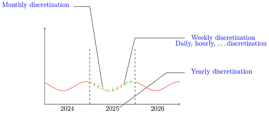
Figure 1. Illustration of the discretization possibilities provided by the continuous-in-time framework.

The layout of this study is structured as follows. Section 2 focuses on the contributions of this study. Section 3 recapitulates the existing discrete mathematical model and how we predict developing the continuous objects. In Section 4, we present various studies related to the continuous framework based on previous theoretical study. Section 5 provides an overview of designing the API with specific goals and constraints. This Section highlights the advanced API mechanisms for building the framework, including time steps and software architecture representing the basis organization of software artifacts. Section 6 covers the implemented methods and objects to demonstrate the computational concept adopted by these mechanisms These implemented algorithms are expressed formally to show the illustrative API purposes. We conclude by summarizing the major points of this study in Section 7.

2 Contexts and contributions

Scientific computing softwares are always implemented using low-level languages, such as C or Fortran, losing the high-level structure, but some of the well-known softwares for computational finance are developed in C++ and C# in the .NET platform. What is challenging in this study is to implement the framework in form of Application Programming Interface (API). Paticularly, one of the central design philosophies of this API is to allow information to be quickly interchanged without great modifications in coding. The implementation is realized in C#, is considered one of the most widely used programming languages, and leads to integrate this API inside SOFI to produce the continuous software tool (Hickey and Harrigan, 2022; Golmohammadi et al., 2023; Hung et al., 2024). The proposed API applies to partial differential equations arising applications in mathematical finance. This API focuses on using parallelism adopted by Microsoft and provided by Task Parallel Library (TPL). This choice is motivated by parallelism with creating benchmarks for parallel programming (Chakkour, 2022, 2024a,b). The covenient using the API is to facilitate the continuous integration (CI) and connection from this interface with external systems. The modern systems involving continuous integration on different platforms and technologies are described in the literature (Gaston et al., 2009; Lima and Vergilio, 2020). The study of Jackson et al. has adoted this CI environment in Lima and Vergilio (2020) to make the software evolution more rapid and cost-effective. The MOOSE (Gaston et al., 2009) project uses the direct continuous integration between one developed framework and all computational applications to make rapid development of high-quality scientific software.

The main contributions in this study classify the API implementation into two libraries, Lemf (Library Embedded Finance) and LemfAN (Library Embedded Finance And Numerical Analysis). Note that LemfAN is an open-source library; however, Lemf remains confidential, particularly its integration in SOFI. Our own philosophy is to allow these libraries to be quickly interchanged without much code change. Each library contains the collection classes and the interfaces which are partially characterized by their properties. The present study aims to give an overview of this API in detail and its design rationale, including the time complexity of all operations (Bossen et al., 2021; Liu et al., 2021). Finally, we will explain some techniques used in the implementation. The purpose of these libraries is to compute loan, reimbursement, and interest payment schemes.

3 Mathematical objects

This short section aims to describe the mathematical objects used in the discrete modeling. These objects involved in the models are sequels and series (Eling and Loperfido, 2020; Marin and Vona, 2023). It means that at an instant n, the state of the modeled system is presented by a large vector U_n, of dimension p. Formally, the financial state at time n+1 is expressed by a recurrence relation which can be written in the following form,

$\begin{array}{l}{U}_{n+1}=F(U_n),\\ \\ U_{n+1}=F(U_n,U_{n-1},\dots ,U_0).\end{array}$

The financial analyses used in this model on contingency tables are within Excel tool. Figure 2 exhibits the data entry in Excel tables and financial trends illustrated in SOFI software. The disadvantages of the discrete models (as described at the beginning of the study) consist in using typical mathematical objects such as sequences and series. Utilizing this approach involves limitations in time and operating redundant objects. Furthermore, there is a restriction to reimplementing the time period at each modeling process. This constraint does not correlate well with the financial reality. In other words, the modeling needs to offer more flexibility with smaller periods. Note that all these objects are exactly of the same nature. Therefore, some objects can be calculated by formulas in the following type,

$\begin{array}{ll}{W}_n={\displaystyle \sum _{m=0}^n}{a}_m{U}_m.& (1)\end{array}$

Figure 2

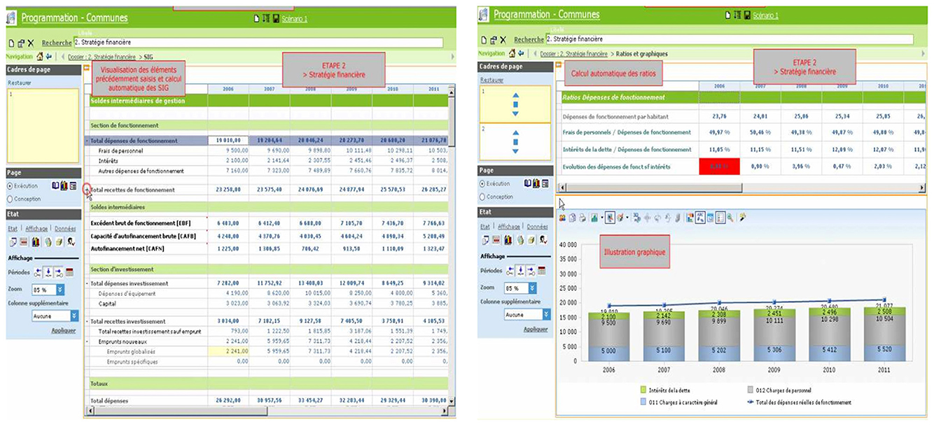
Figure 2. Data entry and financial trends in discrete SOFI software.

The first reflection in building the continuous framework to be carried out is establishing the list of new objects that must be manipulated according to their intrinsic nature. Then, choose the appropriate objects having the best representation. For instance, the summation mentioned in relation (Equation 1) can be replaced by integral, and so on. The concept follows this idea even though it is more complicated than that. The complexity is to determine the suitable space in which the model should be built, and these objects can be consistently operated. This complexity will be detailed mathematically in the next section. Then, the financial variables defined in the framework should be represented by measures and fields as depicted in Figure 2. The reason is that generally the notion of measure is an extension of natural concepts of length, surface, and volume. The purpose is to evaluate the amounts given in monetary units corresponding to sums over time period.

There will be considerable potential financial motivation toward creating and implementing the concept of continuous operators. The Excel-based financial module that executes discreet observation modeling is removed to design a computer module that works efficiently without exchanging Excel data. Consequently, the drawbacks of controlling the time period are solved. Through this research study, we will show how implementing integral operators continuously in the targeted space leads to observing the financial risks with tiny periods. However, a direct comparative performance between the discrete modeling and the developed framework will not occur and is outside the scope of this study. The difficulty is accessing SOFI (Excel data). Moreover, an analogy cannot be made simply by comparing them within the same data. In addition, the discrete-parallelization framework appears complicated due to the data structures, programming features, and invoked drawbacks. Fortunately, the computation mechanism is improved within new sophisticated mathematical objects as illustrated in Table 1, and the limitations of the existing models are provided with various explanations. Both frameworks have different modeling paradigms. The expected performances will be naturally expected without direct comparison.

Table 1

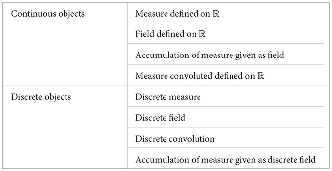
Table 1. Mathematical objects expected to be developed for continuous modeling.

4 Related works

The model building is based on the Radon Measure space $ℳ([t_{\text{I}},{\Theta }_{\text{max}}])$ which is a Banach space over ℝ, supported in $[t_{\text{I}},{\Theta }_{\text{max}}]$, when provided with norm:

$\begin{array}{l}\parallel \psi {\parallel }_{L^{\infty }([t_I,{\Theta }_{max}])}=\underset{t\in [t_I,{\Theta }_{max}]}{\sup }\{|\psi (t)|\},\hfill \end{array}$

The Measure space $ℳ([t_{\text{I}},{\Theta }_{\text{max}}])$ is the space dual ${\mathcal{C}}_c^o([t_{\text{I}},{\Theta }_{\text{max}}])$ of continuous functions defined over $[t_I,{\Theta }_{max}]$. Among $ℳ([t_I,{\Theta }_{max}])$, some measures are absolutely continuous with respect to the Lebesgue measure, and some of them are not. When a given measure $\tilde{m}$ is absolutely continuous, this means that it reads m(t)dt, where t is the variable in ℝ, and m(t) is its density, that is, $\tilde{m}=m(t)dt$. We have defined in Frénod and Chakkour (2016) the variable measures in which their densities are the amounts expressed in monetary unit. Some of these financial variables built in the model can be described as follows. The first one is the Loan Measure ${\tilde{\kappa }}_E$. This variable is defined such that the amount borrowed between times t₁ and t₂ is the following amount:

$\begin{array}{ll}\begin{array}{l}{\displaystyle {\int }_{t_1}^{t_2}{\tilde{\kappa }}_E}.\hfill \end{array}& (2)\end{array}$

The second one is the Capital Repayment Measure ${\tilde{\rho }}_{\mathcal{K}}$. It is defined such that the amount of capital which is repaid between t₁ and t₂ is the following value:

$\begin{array}{ll}\begin{array}{l}{\displaystyle {\int }_{t_1}^{t_2}{\tilde{\rho }}_{\mathcal{K}}}.\hfill \end{array}& (3)\end{array}$

The Repayment Pattern $\tilde{\gamma }$ manifests in the model the way an amount 1 borrowed at t = 0 is repaid. It means that this Pattern $\tilde{\gamma }$ is a measure with total mass which equals 1, that is:

$\begin{array}{ll}{\displaystyle {\int }_{-\infty }^{+\infty }}\tilde{\gamma }=1.& (4)\end{array}$

Loan Measure ${\tilde{\kappa }}_E$ and Capital Repayment Measure ${\tilde{\rho }}_{\mathcal{K}}$ are connected by a convolution operator:

$\begin{array}{ll}{\tilde{\rho }}_{\mathcal{K}}={\tilde{\kappa }}_E\star \tilde{\gamma },& (5)\end{array}$

Linear operator $\mathcal{L}$ is introduced in Chakkour (2017a), and acting on Loan Density ${\kappa }_E\in {\mathbb{L}}^1([t_{\text{I}},{\Theta }_{\text{max}}-{\Theta }_{\gamma }]){{\displaystyle \cap }}^{\text{}}{\mathcal{C}}_c([t_{\text{I}},{\Theta }_{\text{max}}-{\Theta }_{\gamma }])$, and is defined as follows:

$\begin{array}{ll}\mathcal{L}[{\kappa }_E](t)={\kappa }_E(t)-({\kappa }_E\star \gamma )(t)-\alpha {\displaystyle {\int }_{t_{\text{I}}}^t({\kappa }_E-{\kappa }_E\star \gamma )(s)};ds.& (6)\end{array}$

The operator $\mathcal{D}:{\mathbb{L}}^1([t_{\text{I}},{\Theta }_{\text{max}}]){{\displaystyle \cap }}^{\text{}}{\mathcal{C}}_c([t_{\text{I}},{\Theta }_{\text{max}}])\to {\mathbb{L}}^1([t_{\text{I}},{\Theta }_{\text{max}}])$ is acting on the Initial Debt Repayment Density ${\rho }_{\mathcal{K}}^{\text{I}}$, defined as:

$\begin{array}{ll}\mathcal{D}[{\rho }_{\mathcal{K}}^{\text{I}}](t)=-\alpha {\displaystyle {\int }_t^{{\Theta }_{\text{max}}}{\rho }_{\mathcal{K}}^{\text{I}}}(s);ds-{\rho }_{\mathcal{K}}^{\text{I}}(t).& (7)\end{array}$

We have discussed the inverting of the operators $\mathcal{L}$ and $\mathcal{L}+\mathcal{D}$ on the space of square-integrable functions defined on a compact (respectively, $\tilde{\mathcal{L}}$ and $\tilde{\mathcal{L}}+\tilde{\mathcal{D}}$ when they are extended to radon measure space) in previous studies (Chakkour and Frénod, 2016; Chakkour, 2017b, 2019, 2023). The ill-posedness arising in this framework is examined in these spaces in order to obtain interesting and useful financial solutions and to forecast the budget for future financial plans well.

To emphasize the mathematical aspects of duality and to simplify the notations, the duality bracket will be used to represent the integration of a continuous function with respect to the radon measure over ℝ. In practice, all the building measures are defined on ℝ. In reality, implementing this theory seems to be easy, but the difficulty consists of having continuous piecewise functions that are continuous with superior values in place of continuous functions. For instance, the amounts presented in relations (Equations 2, 3) via integral operator can be presented, respectively, as $<{\tilde{\kappa }}_E,{\mathrm{𝟙}}_{[t_1,t_2]}>$ and $<{\tilde{\rho }}_{\mathcal{K}},{\mathrm{𝟙}}_{[t_1,t_2]}>$.

5 Design and concept of computation in API

This section introduces the architectural designs and styles. This also illustrates the development process for describing the API layers. The programming paradigms govern these layers. The application diagram below will show some assembled and configured instances of abstractions that are used to inter-communicate between them. These concrete layers are viewed in terms of the code base to manage and control the instantiation of domain abstractions. Next, abstractions are displayed by compatible ports according to the class diagrams.

5.1 Physical view

The design of the API is shared into tow layers which are a low level and high level. Figure 3A illustrates these two levels. The high level is created for business reasons. The financial variables are computed in high level, and next remain accessible for the SOFI users. Note that low level does not use the high one. We say that high level implements its low. The low and high levels contain non-discrete measures and fields, and discrete measures and fields on ℝ. Depending on the targeted computations, some of them in high level need discretization. For instance, if the aim is to discretize a measure in the high level, its copy is built in low level. Next, it is discretized to rise up its values to high level.

Figure 3

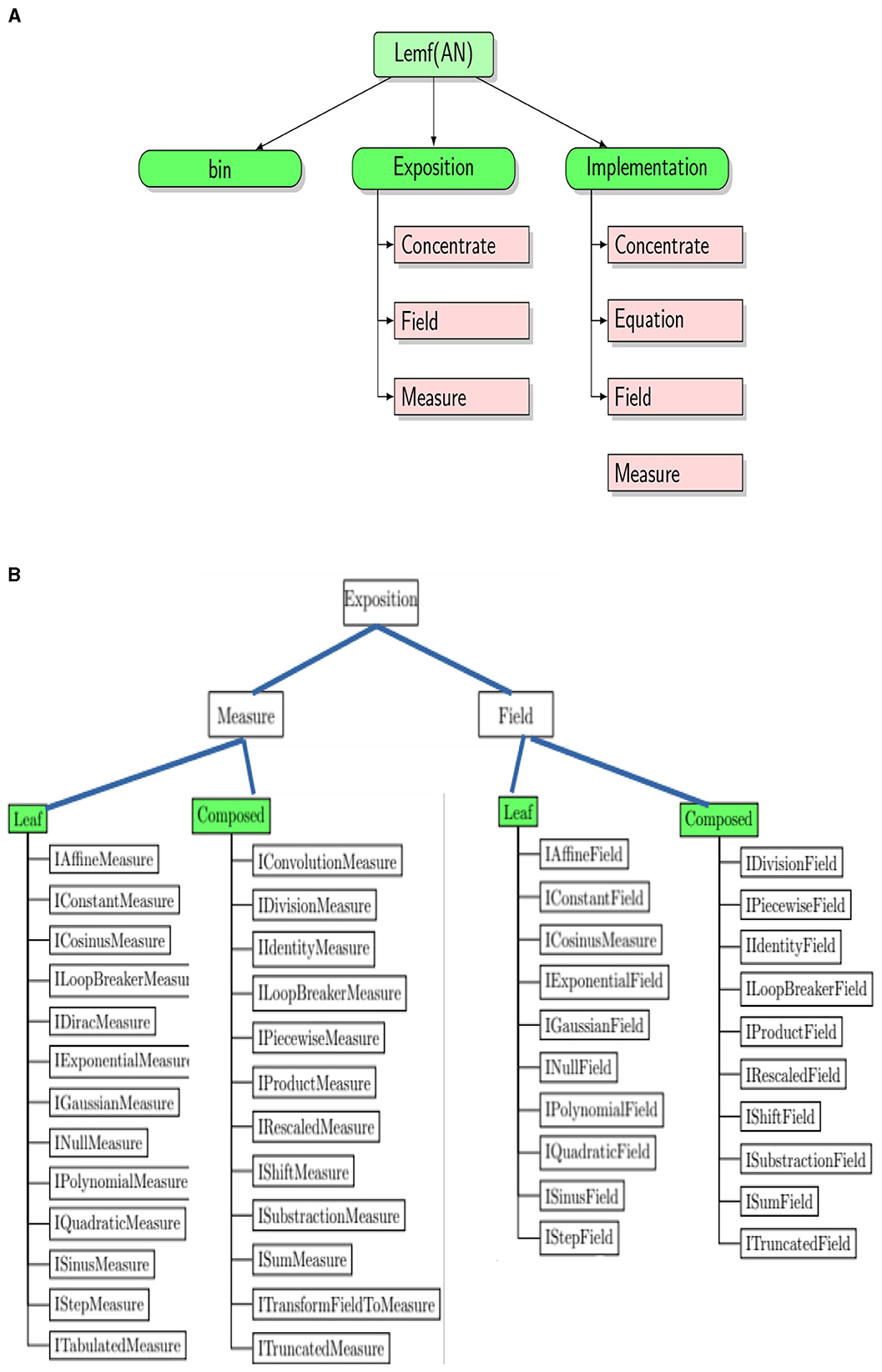
Figure 3. The physical view illustrating the API design. (A) Decomposition of each application layer into three parts. (B) Partial application diagram expressed by container-based exposition.

Class diagrams are powerful tools that boost relationships between classes, averting them from being good abstractions. Since many objects are presented in the application, it is not easy to use this tool to show them. Figure 3 identifies the architectural elements of financial processing solutions of the framework API by exposing their functionality, which is divided into two figures. The content of the application layer can be summarized in Figure 3A. Each library has three folders. This decomposition gives specific characteristics and facilities for physically viewing the API. The logical view (Spray et al., 2021; Górski, 2022) is then separated by differentiating interfaces and implementations. In brief, what objects can be exposed, and what can be implemented? Figure 3B shows the programming paradigms of the Exposition folder. This folder contains simple interfaces for each measure and field. The folder associated with Exposition is named Implementation. It defines explicitly the measure and field objects that implement the interfaces. To define each class, a programming paradigm is used and implemented as an interface. We build in Chakkour and Frénod (2016) a numerical approach to concentrate a given measure as a sum of Dirac masses. This new approach is named Concentrate as illustrated in Figure 3A and aims to enrich the model.

For leveraging the commonly applied utility computing paradigm, the intended architecture has to be laid out robust resources. The API contains a set of connected classes and objetcs involving sophisticated computed mechanisms (as a service factory). A part of reflective information from these objetcs is presented in Figure 4 to facilitate its visual perception. The objective here is to give the concrete implementation details for the API by describing its architecture. The internal architecture of librairies can be visualized as layers, as shown in this figure, that are connected for forming the API. The computation in the library Lemf is defined as a graph where the terminal nodes are measures or fields, and where the non-terminal nodes are operations. Then, Lemf allows us to build its dynamically. These graphs are realized by the abstract factory class named AbstractFactor. This class contains an interface that is responsible to create a factory of related objects without explicitly specifying their classes. Each generated factory can give the objects as per the Factory pattern. This is aimed at creating measures, fields, and operations, which are used by interfaces. Recall that abstract classes are classes whose implementations are not complete and that are not instantiable. These classes as illustrated in Figure 5 are created in the library LemfAN to characterize simple measures (AbstractLeafMeasureAN) and composed measures (AbstractComposedMeasureAN). Abstract classes AbstractLeafMeasureAN and AbstractComposedMeasureAN inherit from the class AbstractMeasureAN since simple and composed measures are generally measures.

Figure 4

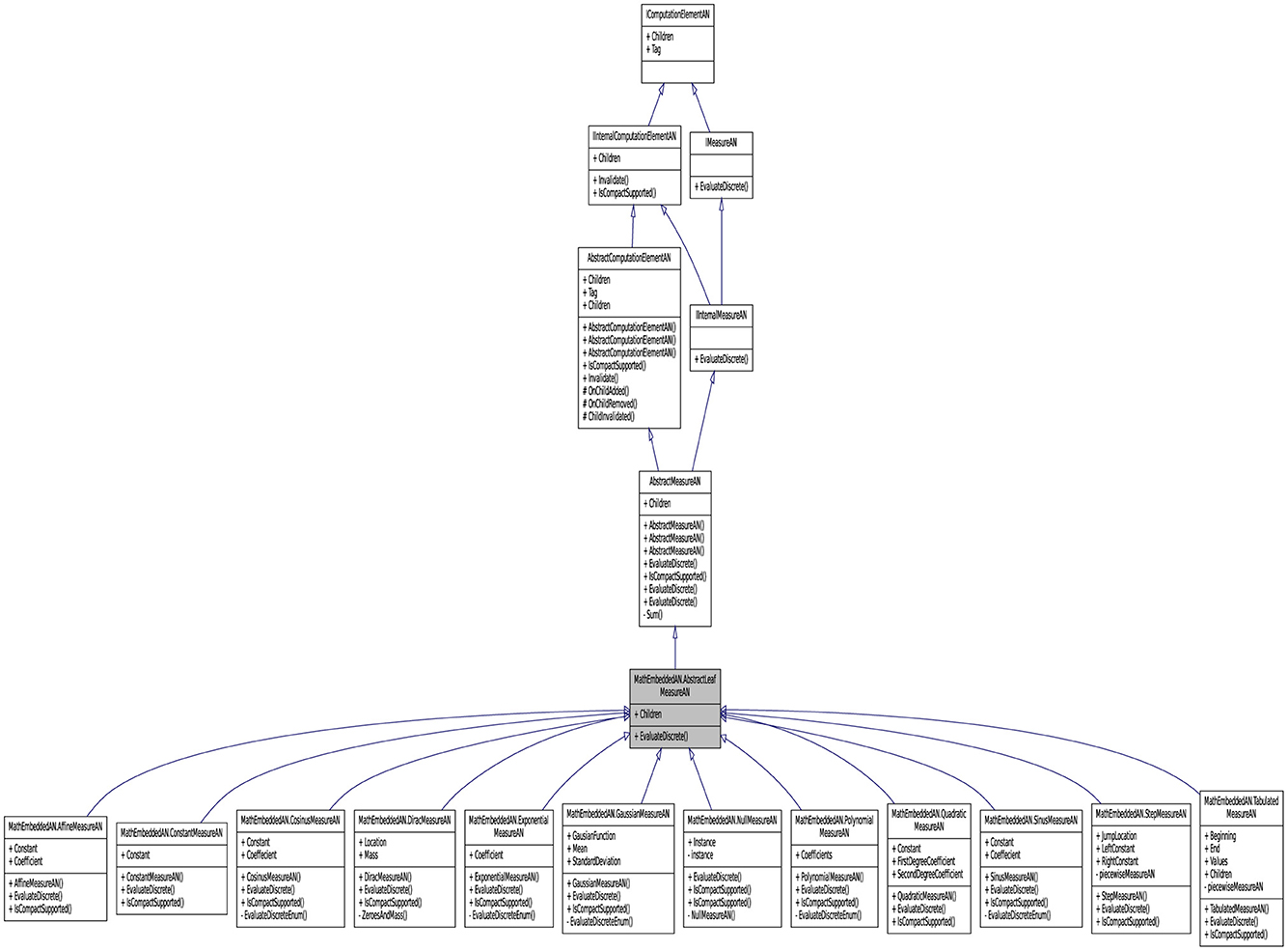
Figure 4. Partial application diagram expressing classes and objetcs including their properties for showing the inheritance paradigm of LeafMeasureAN.

Figure 5

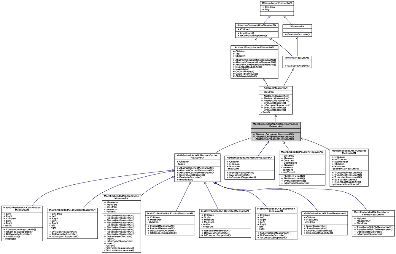
Figure 5. Partial application diagram expressing classes and objetcs including their properties for showing the inheritance paradigm of ComposedMeasureAN.

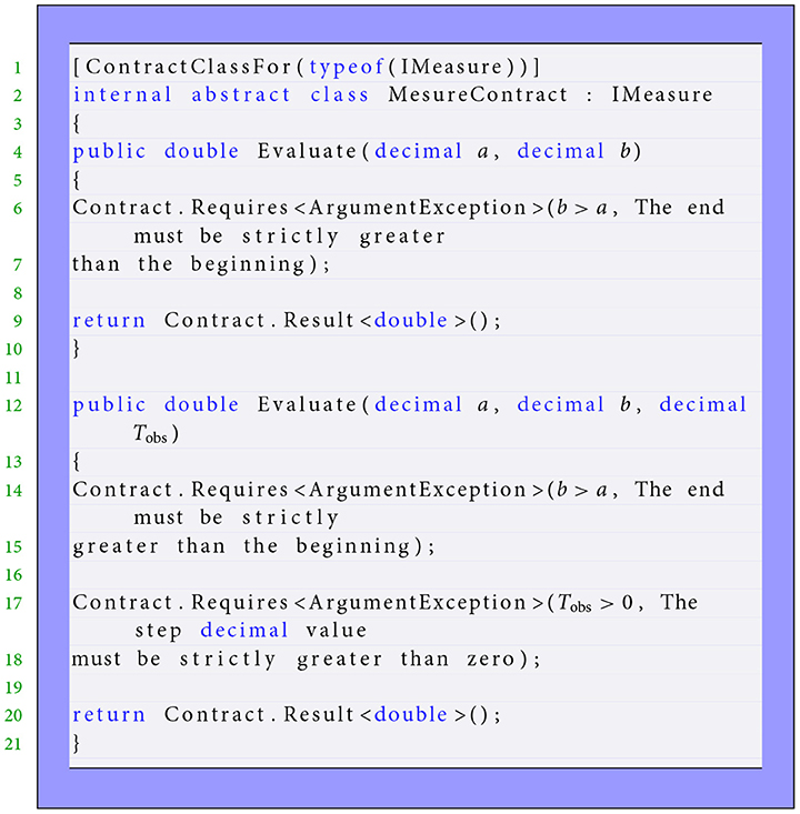
One of the great challenges that includes developing the API components is interacting effectively with the financial feeds and handling the different types of data formats in SOFI modules. Some important interfaces used in the API are described below. For instance, the interface IMeasureAN (see Listing 1) implements all measures in low level and provides a method EvaluateDiscrete. This method allows discretization of a non-discrete that returns a task containing ${\mathcal{N}}_a^b$ discrete values. Task < > is a generic class where the associated action returns a result to encapsulate the abstraction of a computation. The idea of creating the interface IMeasureAN is to spawn one task stored in an array of values. The parallel discrete measures and fields in this level are based on the concept of a task. Using TPL permites to entail execution and development speed, as shown in Leijen et al. (2009). In addition, the interface IMeasure implements all high-level measures. It provides a method Evaluate returning to a value. The code contracts, such as MesureContract, are applied to these interfaces for checking the constraints and signaling violations. The aim is to respect constraints imposed in modeling and then prevent users from using convenient special postconditions. The code snippets in Listings 2, 3 illustrate the representatives of this design Interface pattern and its contract.

Listing 1

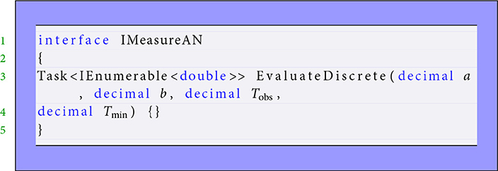
Listing 1. The interface IMeasureAN.

Listing 2

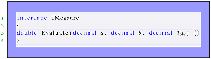
Listing 2. The interface IMeasure.

Listing 3

Listing 3. The code contracts.

As illustrated in Figure 6, the convolution operator is based on the Fast Fourier Transform (FFT). The FFT has been applied using the inbuilt Math.NET Numerics (Math.net package, n.d.) that is an excellent scientific library written entirely in C#. This library supports two linear integral transforms: The discrete Fourier and Hartley transforms. Both of them are strongly localized in the frequency spectrum. The .NET platform contains the Iridium and Neodym packages, including the Math.NET, which handles complex values. In reality, the concept of data parallelism through the TPL represents an asynchronous operation resembling a thread item with a higher level of abstraction. The partial code (Listing 4) shows a part complex pattern of data parallelism from a convolution operator and demonstrates the mathematical implementation illustrated in equalities (Equations 4–52). The first step to detecting the pattern is to use Factory.StartNew, which yields the task creation and task starting operations. The leftTask and rightTask correspond to the computation tasks defined, respectively, by the discretization of the left-hand Left and right-hand Right measures on the convex hull of their supports. These convex hulls are presented by leftAxeSegment and rightAxeSegment respecting the definition (Equation 10). The method IsCompactSupported is implemented to determine the convex hulls for each measure, particularly for the convolution with two extreme points. The method Parallel.Invoke is a succinct method to create and start leftTask and rightTask and waiting for them. Then, the process is divided into two sub processes (threads) using this method. These tasks are created separately and executed potentially in parallel. These actions are accompanied by completing these discrete measures by zero elements and applying the Fourier Transform operator. Note that the NumericalRecipes flag is used to keep the need for Numerical Recipes compatibility. When a work item has been completed, a targeted vector is computed by element-wise multiplication.

Figure 6

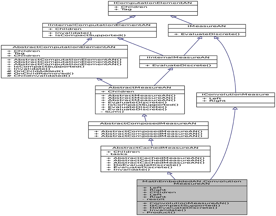
Figure 6. UML profile diagram showing the pattern design of the convolution operator.

Listing 4

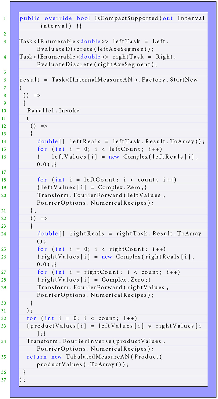
Listing 4. The convolution operator.

The class ConstantMeasureAN defines the constant measure in low level and inherited from two interfaces AbstractLeafMeasureAN and IConstantMeasure. Another class of inheritances follows the same way of the interface behavior. For example, this definition states that the class based on the Dirac measure is a common visible interface AbstractLeafMeasureAN and also a part of the interface information IDiracMeasure. The following code fragments (Listing 5) show the implementation that an instance of theses classes are created.

Listing 5

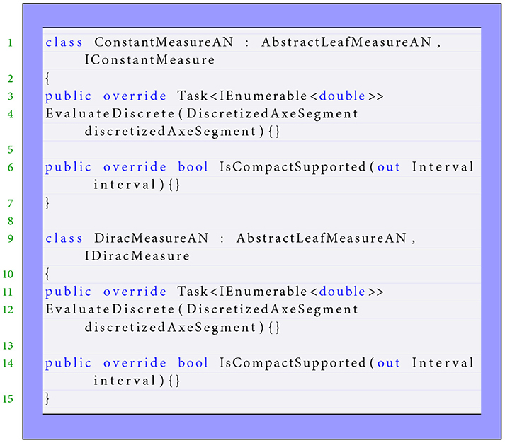
Listing 5. The constant and Dirac measures.

5.2 Numerical simulation using the financial API

This part is devoted to interpreting the continuous-in-time framework financially via the API (Uddin et al., 2020; Naqvi et al., 2023). We will adopt the financial point of view according to what developed as a mathematical operator introduced in Section 4. The API consistency is analyzed financially to interpret it with more explanations using a simplified problem. Now, we turn to richer API simulations. The simulation presented in Figure 7 via Listing 6 (shared into three diagrams) shows the action of Repayment Pattern $\tilde{\gamma }$, which is a combination of seven Dirac measures on Loan Measure ${\tilde{\kappa }}_E$, which is a combination of five Dirac masses. This pattern is an aggregate of three Dirac masses having the same mass $\frac{5}{19}$, located at various instants 0.3, 0.4, and 0.5; the other four Dirac masses have the same mass $\frac{5}{19}$ at instants 0.25, 0.35, 0.45, and 0.55. The measure $\tilde{\gamma }$ can be written in the following form,

$\begin{array}{l}\tilde{\gamma }=\frac{5}{19}\times ({\delta }_{t=0.3}+{\delta }_{t=0.4}+{\delta }_{t=0.5})\\ +\frac{1}{19}\times ({\delta }_{t=0.25}+{\delta }_{t=0.35}+{\delta }_{t=0.45}+{\delta }_{t=0.55}).& (8)\end{array}$

Figure 7

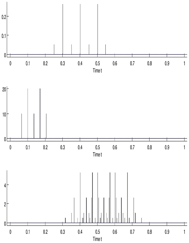
Figure 7. Financial simulation via API convolution operator. The variables are the concentrated measures, where $\tilde{\gamma }$ is represented at the top, ${\tilde{\kappa }}_E$ in the middle, and ${\tilde{\rho }}_{\mathcal{K}}={\tilde{\kappa }}_E\star \tilde{\gamma }$ at the bottom.

Listing 6

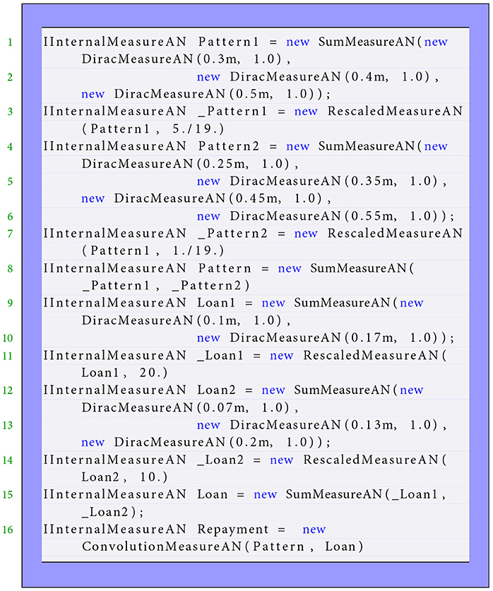
Listing 6. The convolution operator modeling the financial simulation shown in Figure 7.

Note that the defined $\tilde{\gamma }$ satisfies the following variant of relation (Equation 4), since it expresses the way an amount 1 borrowed at the initial instant is repaid. The middle diagram illustrates the loan measure, which is shared into two pieces. The first is expressed by borrowing the amount 20 at instants 0.1 and 0.17. The second consists of borrowing the amount 10 at instants 0.07, 0.13, and 0.2. Formally,

$\begin{array}{ll}{\tilde{\kappa }}_E=20\times ({\delta }_{t=0.1}+{\delta }_{t=0.17})+10\times ({\delta }_{t=0.07}+{\delta }_{t=0.13}+{\delta }_{t=0.2}).& (9)\end{array}$

This convolution result is computed using the formula (Equation 5) and is presented in the bottom diagram. It is also the combination of various concentrated measures that can be approached by a density measure. The Repayment Plan associated with Loan Measure ${\tilde{\kappa }}_E$ and Repayment Pattern Measure $\tilde{\gamma }$ is constituted by four parts of repayments described as follows:

• The first consists of the reimbursement of amount $\frac{100}{19}$ located at instants 0.4, 0.47, 0.5, 0.57, 0.6, and 0.67;

• The second consists of the reimbursement of amount $\frac{20}{19}$ located at instants 0.35, 0.42, 0.45, 0.52, 0.55, 0.62, 0.65, and 0.72;

• The third is associated with the repayment of amount $\frac{50}{19}$ located at instants 0.37, 0.43, 0.47, 0.5, 0.53, 0.57, 0.6, 0.63, and 0.7;

• The last is made of amount $\frac{10}{19}$ at instants 0.32, 0.38, 0.42, 0.45, 0.48, 0.52, 0.55, 0.58, 0.62, 0.65, 0.68, and 0.75.

The presented example written below in API code illustrates well the capability of our model to be used without using the Excel tables to compute the Repayment Plan. This computation is realized without any restriction concerning the time period at which the model is going to be observed. This simulation, named upon “model observation,” can justify that density measures can be used in place of concentrated measures in the form of a combination of Dirac measures. This means that if Loan Measure ${\tilde{\kappa }}_E$ and Repayment Pattern Measure $\tilde{\gamma }$ can be approached by density measures κ_Edt and γdt, then Repayment Density ρ_𝒦dt is an idealization of Repayment Measure ${\tilde{\rho }}_{\mathcal{K}}$ given by equality (Equation 5) over the time interval.

5.3 Time step mechanism

We generate the unidimensional mesh named DAS (Discretized Axe Segment) for two purposes. The first is to better structure the low level, providing an efficient way to interact with the next level along simple protocols. The second is to calculate the discrete convolution because of inability to compute it with variable discrete step by the Fast Fourier Transform operator. The Mesh DAS associated with the discrete step T_dM is defined by a set of points (_xk)k∈ℤ that are its multiple,

$\begin{array}{ll}{\text{DAS}}_{{\text{T}}_{\text{dM}}}=\{x_k=k\times T_{\text{dM}},k\in \mathbb{Z}\}.& (10)\end{array}$

This part is devoted to define time steps that are involved in the models and the relations between them. Figure 8 depicts the different time steps used in the software mechanism within scale modeling. Setting out a financial framework in time is the central element influencing financial economic behavior. This framework should be implemented to answer a question that first sets the whole time period of interest. It consists of considering various parameter times needed. Then, this strategy goes on to compute the values of all financial quantities following the time process. The authors describe in Guseinov (2003) the time scales to integrate density over interval. The variable T_min is introduced to mean the time scale below which nothing coming from the model will be observed. Specifically, we say that a measure $\tilde{m}$ is observed over time interval [t₁, t₂] if,

$\begin{array}{ll}{\displaystyle {\int }_{t_1}^{t_2}}\tilde{m},& (11)\end{array}$

Figure 8

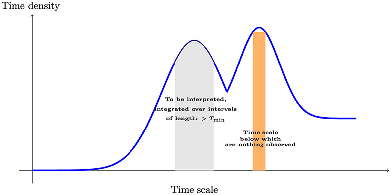
Figure 8. Various time steps defined in the continuous-in-time financial modeling.

is calculated. We will always choose times t₁ and t₂ such that t₂−t₁>T_min. In order to observe models, we need an observation step T_obs which is strictly superior than T_min

$\begin{array}{ll}{T}_{\text{obs}}>T_{\text{min}}.& (12)\end{array}$

The discretization step T_dM in the low level is defined as a smaller step than minimal observation step T_min to discretize measures.

$\begin{array}{ll}{T}_{\text{dM}}\le T_{\text{min}}.& (13)\end{array}$

In practice, the discrete step T_dM is fixed as,

$\begin{array}{ll}{T}_{\text{dM}}=\frac{T_{\text{min}}}{20}.& (14)\end{array}$

The quantity n_D is defined as the observation step T_obs in term of the step T_dM,

$\begin{array}{ll}\begin{array}{l}{n}_D=\lfloor \frac{T_{\text{obs}}}{T_{\text{dM}}}\rfloor .\hfill \end{array}& (15)\end{array}$

The field is defined as continuous function by superior value. It is evaluated between inferior value a and superior value b with discrete step T_dF satisfying:

$\begin{array}{ll}0<T_{\text{dF}}<b-a.& (16)\end{array}$

Integrating a given measure m_d in low level between inferior bound a and superior bound b with minimal observation step T_min consists of integrating it between new inferior bound x_a and new superior bound x_b with discrete step T_dM that verify,

$\begin{array}{ll}{x}_a=n_a\times T_{\text{dM}},x_b=n_b\times T_{\text{dM}}.& (17)\end{array}$

In which the integers n_a and n_b are defined as,

$\begin{array}{ll}{n}_a=\lfloor \frac{a}{T_{\text{dM}}}\rfloor ,n_b=\{\begin{array}{l}\frac{b}{T_{\text{dM}}}\text{ if }{T}_{\text{dM}}\text{ is divisible by }b,\\ \lfloor \frac{b}{T_{\text{dM}}}\rfloor +1\text{ else.}\end{array}& (18)\end{array}$

Denoting by ${\mathcal{N}}_a^b$ the number of subintervals of interval [x_a, x_b] defined as,

$\begin{array}{ll}{\mathcal{N}}_a^b=n_b-n_a.& (19)\end{array}$

For any integer j from 1 to ${\mathcal{N}}_a^b$, we define ${(n_a+j-1)}^{\mathrm{\text{nd}}}$ discrete value of measure m_d, its integration between inferior bound (n_a+j−1) × T_dM and superior bound (n_a+j) × T_dM,

$\begin{array}{ll}\forall j\in 〚1;{\mathcal{N}}_a^b〛,m_d(n_a+j-1)={\displaystyle {\int }_{(n_a+j-1)\times T_{\text{dM}}}^{(n_a+j)\times T_{\text{dM}}}}{m}_d.& (20)\end{array}$

The quantity $m_d^{\mathrm{\text{obs}}}(i)$ is defined as observed discrete measure over interval with time length T_obs, the integration of measure m_d between inferior bound n_a×T_dM+(i−1) × T_obs and superior bound n_a×T_dM+i×T_obs.

$\begin{array}{ll}\begin{array}{l}\forall i\in 〚1;\lfloor \frac{{\mathcal{N}}_a^b}{n_D}\rfloor 〛,m_d^{\text{obs}}(i)={\displaystyle {\int }_{n_a\times T_{\text{dM}}+(i-1)\times T_{\text{obs}}}^{n_a\times T_{\text{dM}}+i\times T_{\text{obs}}}{m}_d.}\hfill \end{array}& (21)\end{array}$

This integral can be decomposed with Chasles relation,

$\begin{array}{ll}\begin{array}{l}\forall i\in 〚1;\lfloor \frac{{\mathcal{N}}_a^b}{n_D}\rfloor 〛,m_d^{\text{obs}}(i)={\displaystyle \sum _{k=1}^{k=n_D}{\displaystyle {\int }_{(n_a+k-1)\times T_{\text{dM}}+(i-1)\times T_{\text{obs}}}^{(n_a+k-n_D)\times T_{\text{dM}}+i\times T_{\text{obs}}}{m}_d.}}\hfill \end{array}& (22)\end{array}$

Next, this integral can be simplified as,

$\begin{array}{ll}\begin{array}{l}\forall i\in 〚1;\lfloor \frac{{\mathcal{N}}_a^b}{n_D}\rfloor 〛,m_d^{\text{obs}}(i)\simeq {\displaystyle \sum _{l=1+(i-1)\times n_D}^{l=i\times n_D}{\displaystyle {\int }_{(n_a+l-1)\times T_{\text{dM}}}^{(n_a+l)\times T_{\text{dM}}}{m}_d.}}\hfill \end{array}& (23)\end{array}$

Equalities (Equations 20, 23) yield that the observed value $m_d^{\mathrm{\text{obs}}}(i)$ is a sum of all discrete values m_d(n_a+l−1) for an integer l from 1+(i−1) × n_D to i×n_D,

$\begin{array}{ll}\begin{array}{l}\forall i\in 〚1;\lfloor \frac{{\mathcal{N}}_a^b}{n_D}\rfloor 〛,m_d^{\text{obs}}(i)\simeq {\displaystyle \sum _{l=1+(i-1)\times n_D}^{l=i\times n_D}{m}_d(n_a+l-1).}\hfill \end{array}& (24)\end{array}$

According to equality (Equation 24), there are two cases of calculating the observed values $m_d^{\mathrm{\text{obs}}}$. The first case consists in computing them when ${\mathcal{N}}_a^b$ is divisible by n_D. The second case consists in computing them, when ${\mathcal{N}}_a^b$ is not divisible by n_D using the simplified form,

$\begin{array}{ll}{m}_d^{\text{obs}}\left(\lfloor \frac{{\mathcal{N}}_a^b}{n_D}\rfloor +1\right)\simeq {{\displaystyle {\displaystyle \sum _{k=n_D\times \lfloor \frac{{\mathcal{N}}_a^b}{n_D}\rfloor +1}^{k={\mathcal{N}}_a^b}{m}_d(n_a+k-1).}}}^{\text{}}& (25)\end{array}$

5.4 Testing and performing the API

Unit tests are an essential part of software development. One goal in test data generation is to maximize coverage on all public, protected, and package-private methods. In our API, a special strategy has been proposed to generate tests. This strategy consists of reducing the number of tests and rising the code coverage. It is based on a technique named search-based software testing (SBST) (Perera et al., 2022; Ren et al., 2023), which is famous in the optimized test generation. This technique is similar to Genetic Algorithms (GAs) (Sivanandam et al., 2008). The implementation is improved by attempting the higher coverage result in more detected errors as illustrated in Figure 9A. This result presented in form of table demonstrates that our technique significantly outperforms testing tools in terms of code coverage achieved by 96.4% successful tests. This test generation technique has been successfully employed in Gao et al. (2020) and Golmohammadi et al. (2023). This proportion of covering significant parts from library allows for providing effective protection against bugs.

Figure 9

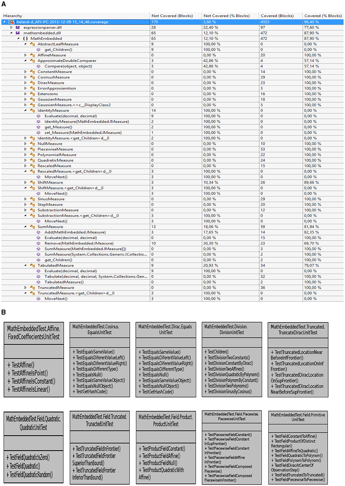
Figure 9. Schematic designs show the creation of unit test (B) suites for object-oriented classes with the anticipated improvements in terms of code coverage (A).

The system tests associated with Lemf/LemfAN are created to enhance test generation without any coverage criteria. Then, each test is structured according to the name of the measure/field and theme as depicted in Figure 9B. This figure highlights a tangible positive correlation from the coverage measure in Figure 9A regarded as an adequate indicator of test sufficiency. For instance, a test named FixedCoeffecientsUnitTest aims to test the constructor firstly, next to check when the affine measure will be constant or linear or reduced to a point with respect to the Lebesgue measure. We have designed suitable unit tests for the test generation to evaluate more existing test cases. Consider testing the Dirac measure that consists of evaluating the mass in term of integration bounds and localization. The effective sets of unit tests are implemented to manage different properties and avoid easily being captured by any individual structural coverage criterion. A reasonable test suite indeed covers all statements of a class, even private methods, indirectly. In addition, the unit tests concerning the Quadratic field are structured into three tests, TestFieldQuadraticIsZero(), TestFieldQuadratic(), and TestFieldQuadraticRandom(). The first aims to evaluate the field when the three coefficients are null. However, the second consists of testing the field when the coefficients are not null. The last leads to selecting these values randomly and independently. The rest of the tests follow the same issues. The performances are guided by a fitness validation that estimates how the coverage results converge for each configuration to its optimality. This optimization concerns the size of the resulting test suite in terms of the number of lines of code and unit tests. Note that without increasing the test suite size, our experiments state that the function coverage suite may grow up to 97% tested code.

We will describe hereafter in the end how to solve the ordinary differential equation, see Equations 61–63. This equation relates the Current Debt Field 𝒦_RD to others measures as ${\tilde{\kappa }}_E$ and ${\tilde{\rho }}_{\mathcal{K}}$. Various rapid implementations of interpolation operators applied at field, constant, linear, and quadratic are presented. The code snippets in Listing 7 test the solved equation in unit testing by comparison. Note that the constant interpolation is set to interpolate the field 𝒦_RD. We can check the method output numerically for three testing purposes and then call the routine subjected to satisfy the computation case. The first test is designed when all involved measures are null, which leads to a comparison with the resulting null field. The second in the middle shows the action of Loan Measure ${\tilde{\kappa }}_E$ which is Dirac mass having the total mass located in 2015.2 on truncated measure pattern ${\tilde{\rho }}_{\mathcal{K}}$. This pattern is one piece consisting of a borrowing amount of 0.25 on the period time [2, 6]. When these measures are provided and evaluated between 2014 and 2024, our API computes the field 𝒦_RD. The last is tested Loan Measure ${\tilde{\kappa }}_E$ which is a sum of two Dirac masses. The first Dirac mass is of mass one at a time 2015.2, and the second one is of mass 2 at time 2016.3. Over the same time period, the field 𝒦_RD is expressed in a monetary amount within 11.

Listing 7

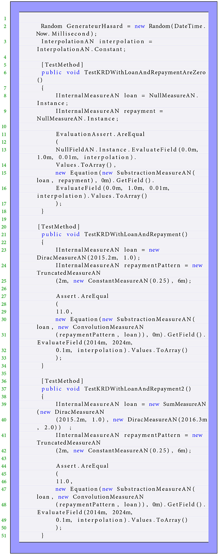
Listing 7. The equation modeling Current Debt Field in low level.

5.5 Computing the convex hull of measures

In this part, we study a practical algorithm for computing an approximate convex hull of some measures. The convex hull of a point set is defined to be the smallest convex set containing these points. Because all our measures are compacted support, the convex hull is used to compute the interval that convolution operator should be discretized. Many aspects of computing convex hulls have been discussed in the literature (Seidel, 2017; Alshamrani et al., 2020; Knueven et al., 2022). A novel pruning-based approach is presented in Masnadi and LaViola (2020) and Keith et al. (2022) for finding the convex hull using parallel algorithms. Our proposal approach is simply based on calculating the final convex hull using the loading extreme points. These points are determined by the maximum and minimum approach. Assuming that the support of measure $\tilde{f}$ can be written as a finite union of two-by-two disjoint closed interval ([_{ai, bi])0 ≤ i ≤ n}. In which n is an integer, and each interval [a_i, b_i] should not be reduced to an empty singleton. Formally,

$\begin{array}{ll}\text{Supp}(\tilde{f})={\displaystyle \bigcup _{i=0}^n}\left\{x\in \left[a_i,b_i\right],a_i\le b_i,f(x)\ne 0\right\}.& (26)\end{array}$

Then, the convex hull of this support is given by,

$\begin{array}{ll}\text{CV}(\text{Supp}(\tilde{f}))=[\underset{0\le i\le n}{\min }{a}_i,\underset{0\le i\le n}{\max }{b}_i].& (27)\end{array}$

We would like to illustrate formula (Equation 27) in case of sum measure described in the next section. This measure is the sum of two Dirac measures. The first Dirac is of mass m₁ localized at time p₁, and the second Dirac is of mass m₂ localized at time p₂. Assuming that masses m₁ and m₂ are not null, such that locations p₁ and p₂ satisfy the condition (Equation 33). This approach is implemented using the method IsCompactSupported for various measures in the API and yields in this situation,

$\begin{array}{ll}\text{Supp}(\tilde{f})=\left\{p_1\right\}{{\displaystyle \cup }}^{\text{}}\left\{p_2\right\},\text{CV(Supp}(\tilde{f}))=[p_1,p_2].& (28)\end{array}$

The purpose now is to maintain some actions and dualities concerning the implementation to provide much resilience in the API. The theory of integration of a piecewise continuous function with respect to the Dirac measure is very complex and undefined. Denoting by δ_p the Dirac measure is localized at point p, which can be interpreted in the framework as the concentrated action or payment. For instance, integrating the continuous piecewise function 𝟙_{]−∞, p]} or 𝟙_{[p, +∞[}, which are fields with respect to the Dirac measure δ_p,

$\begin{array}{ll}{\displaystyle {\int }_{-\infty }^{+\infty }{\mathrm{𝟙}}_{]-\infty ,p]}}d{\delta }_p(x)\text{ or }{\displaystyle {\int }_{-\infty }^{+\infty }{\mathrm{𝟙}}_{[p,+\infty [}}d{\delta }_p(x),& (29)\end{array}$

yields to an undetermined value. Nevertheless, ${\int }_{-\infty }^{+\infty }d{\delta }_p(x)$ could be computed and equal to 1. This is due to the difficulty for reporting the dual of vector space of continuous piecewise function with a finite number of pieces, continuous with superior values. Furthermore, the action of Dirac measure δ_p on fields ]−∞, p] and [p, +∞[, the product of the same measure δ_p by these fields, is also undefined. The Interest Payment Measure ${\tilde{\rho }}_{\mathcal{I}}$ is related to the Current Debt Field 𝒦_RD which is a function that, at any time t, gives the capital amount still to be repaid by a proportionality relation, that is, ${\tilde{\rho }}_{\mathcal{I}}=\tilde{\alpha }{\mathcal{K}}_{RD}(t)$, in which $\tilde{\alpha }$ is the loan rate measure. Given a regular function ϕ, and according to these invoked numerical problems, the value of these actions should be defined consistently with making a choice about Dirac measure δ_p given as,

$\begin{array}{ll}<{\delta }_p,\varphi >={\displaystyle \underset{x\to p^{+}}{lim}}\varphi (x).& (30)\end{array}$

Relation (Equation 30) makes consistently acting Dirac measure δ_p on a set of fields.

The method IsCompactSupported defined in each class of low layer has been briefly introduced before. It is aimed in computing the convex hull for each measure according to equality (Equation 27). The code fragments (Listings 8, 9) indicate the extracted source programs from class definitions Dirac-Piecewise measures to implement this method. The Dirac measure presents a particular case to follow this definition. When the Dirac mass is not null, the support is reduced to its location. Then, the convex hull of the location point is enlarged to define an interval containing this location.

Listing 8

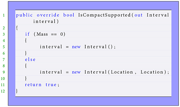
Listing 8. The convex hull of Dirac measure in low level.

Listing 9

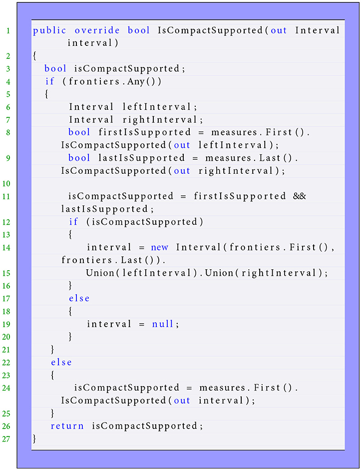
Listing 9. The convex hull of piecewise measure in low level.

5.6 Performances

After describing the design and implementation of our API library, we will provide an example of its use and evaluate its performance. Note that depending on the adequate number of threads, however, the library can be currently executed only on some tasks in parallel and the rest sequentially. The convenience of choosing this structured parallelism consists of that implementation has many freedom parameters in selecting the most efficient scheduling that processes all tasks in the most brilliant way possible. Given the continuous improvements, the API is executed on threads using the TPL library. This makes it easy to take advantage of potential parallelism. Let us compare the performance of the convolution operator in which the code fragments (Listing 4) show shortly a fairly sophisticated implementation. Figure 10 exhibits the relative speedup obtained on a sixty-four-core machine relative to running in parallel with the convolution block. In this experiment, we vary the number of processors from 1, 4, 8, 16, 32, to 64 to investigate the method's speed (Guo et al., 2023; Prichard and Strasser, 2024; Schryen, 2024). Then, we will compare how each method with and without TPL is performed in terms of speed with varying processor sizes. The presented benchmarks illustrate significant speedup, presenting the performance benefit, including runtime. The data structures explicitly take the convoluted properties need more resources for memory models. This was able to achieve great speedup when a number of feature maps are of considerable size. When this number is large, the modern convolutional networks using FFT are accelerated by significant factor of speedup (Cheng et al., 2023; Wang et al., 2023), as expected in Figure 10. In TPL, the particular pattern is captured by Invoke to launch the computed convolution using several parallel operations. We see that parallelism parts are dominant, and the speedups are important until they are four times faster on eight processors. The Fourier Transform via the Math.NET Numerics library demonstrates that TPL can offer performance advantages relative to our environment and application (Lin et al., 2020; Huang et al., 2021).

Figure 10

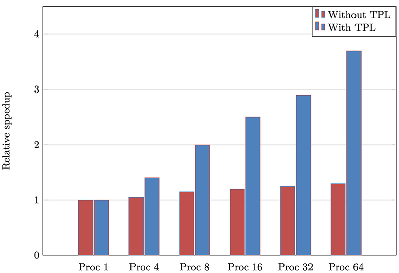
Figure 10. Relative speedup of standard benchmarks from the convolution operator via Math.NET Numerics, given as a function of the number of processors. The tests were run on a 8-socket dual-core Intel Xeon machine with 4Gb memory Windows.

In addition using the Math.NET Numerics library in task parallelism, it contains various distribution properties to evaluate functions. A probability distribution can be parametrized as a normal distribution in terms of mean and standard deviation. The library has its own implementation of the normal distribution that we have used in the API to evaluate it. It is known that it is more stable and faster to compute. We need to implement the normal distribution to define another scenario of continuous data as loan or reimbursement as it is involved in the convolution operator shown in Figure 20.

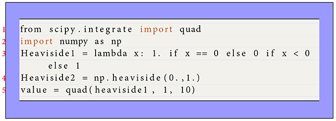
Continuing in correlating the performance of the API with several other commonly used integration function libraries, and find that it achieves competitive performance across a range of tasks. Computational efficiency is a primary objective for the API. There are various libraries available for evaluating numerical integrals (Shaw and Hill, 2021; Kundu and Makri, 2023; Schmitt et al., 2023). This evaluation also concerns discontinuous integral functions via Quad, Trapz, and Simps packages (Weiss and Klose, 2021; Dumka et al., 2022; Tehrani et al., 2024). Note that the Python programming language remains an excellent environment for providing the integration routine to maintain an appropriate level of performance. These packages contain techniques that allow the estimation of definite and indefinite integrals. There are also fairly sophisticated modules as Sympy that helps solve complex mathematical expressions such as differentiation and integration to estimate the values of such empirical functions (Cywiak and Cywiak, 2021; Steele and Grimm, 2024). Again, this package permits for mathematical manipulations of symbols specified by the user The Dirac function is one of them. The code snippets in Listing 10 illustrate the integration process using the package Sympy. The first step implies importing the package.

Listing 10

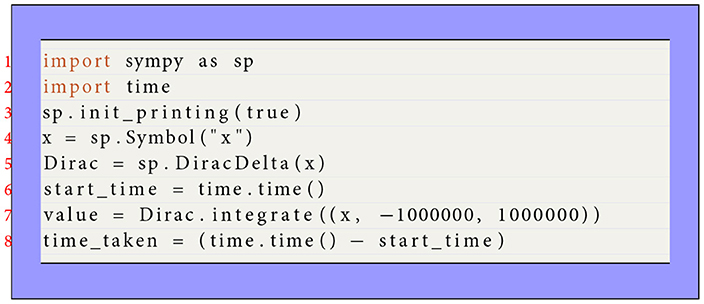
Listing 10. Dirac measure via Sympy.

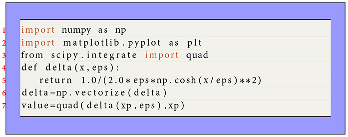
The Dirac function can be defined mathematically as the limit of a sequence of functions, within Lambda instruction, or function definition, that is, rectangular or density functions with the width ϵ and height $\frac{1}{ϵ}$ such that the area is unity as depicted in Figure 11. This figure is run using Python programming language and shared in two diagrams. The left exhibits the approximation representation of the Dirac measure in a rectangle form. The right illustrates this approximation via the Gaussian distribution function with a slightly large peak value. These diagrams are generated using the Python interface. For instance, the Dirac measure can be numerically integrated by calling the module Quad through Scipy.integrate. This predefined function is based on using a technique from the Fortran library QUADPACK. The code snippets in Listing 11 show the integration approach to use this accessible package.

Figure 11

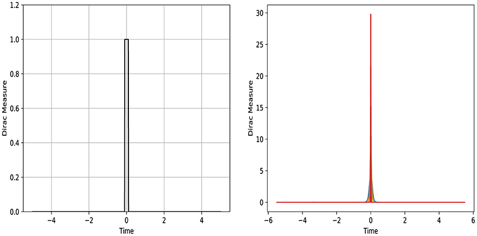
Figure 11. Representation of Dirac measure via Python.

Listing 11

Listing 11. Dirac measure via Quad.

An integration test is run to demonstrate the effectiveness of performance and productivity as depicted in Table 2. It shows the execution time performed to obtain the discrete values from the Dirac measure. The purpose is to compare the performance gains in time by evaluating the discrete Dirac measure mapping from inferior bound to superior bound using our API against the invoked libraries. In this test, the API is executed rapidly in 0.134 s with a large number of iterations in time. The output is stored as the task object containing these discrete values. This is an efficient strategy using the proposed approach, which is justified as follows: The reason consists of using patches of conditional statements such as the implemented method IsCompactSupported, presented in the code Listing 11. The aim is to keep the mass or zero without approximation as some core libraries use it.

Table 2

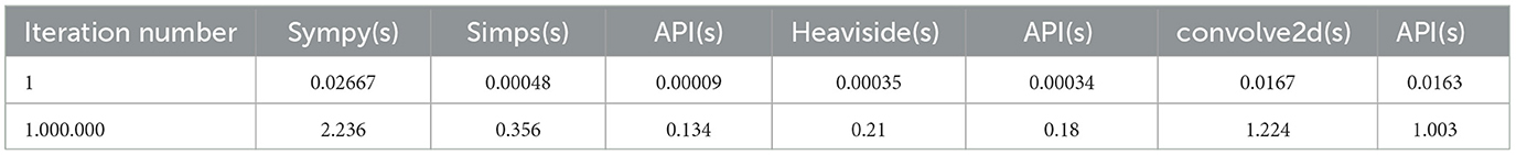
Table 2. Evaluation of Dirac, piecewise, and convolution measures with comparison between various libraries in execution time.

This test is extended to using other functionalities in Python to compare with the improving API method. There is a Heaviside function in Python (see the code Listing 12), which is similarly defined as a piecewise measure with one frontier in our API. Here, the Heaviside function is defined explicitly in the code before the numerical calculation and can be built into Sympy and Numpy. The approximation to the Heaviside function is used enormously in biochemistry and neuroscience (Andreev et al., 2021; Zhou et al., 2023). The Scipy module also provides convolve2d function, which computes the convolution operator of two NumPy arrays. The convolution via this package is considered one of the mathematical operations widely used in signal processing to model two signals to produce a resulting signal. The benchmarking processing time is described in the half-right of Table 2 in which the time usage is recorded. This benchmark is the suite of preliminary tests involving analyzing the standard routines. It compares two commonly used programming languages under two different operating systems. There is evidence of a faster operating system implemented in C# for large discrete-time numbers. It proves that the implementations in C# with respect to Python are the fastest and use the least memory.

Listing 12

Listing 12. Heaviside function via Quad.

Consequently, the API offers good capabilities and powerful tools for analyzing and simulating real-world phenomena in financial engineering (Farimani et al., 2022; Li et al., 2022). It allows for providing numerical solutions to the continuous framework to gain valuable insights, time, and forecasting decisions.

6 Implementation of measures and fields

This section is devoted to implementing two categories of measures: simple and composed. The explicit integration of some simple measures is provided. The integration of composed measures can be expressed explicitly in terms of the integration of simple ones. The simple measure is a collection of measures such as the constant, affine, quadratic, polynomial, exponential, and Dirac. It can be absolutely continuous with respect to Lebesgue measure λ_Lebesgue or cannot be absolutely continuous with respect to the Lebesgue measure λ_Lebesgue as Dirac measure. For instance, the constant measure is created to borrow uniformly over a time interval. The constant density m_Constant is defined which is equal to a real C independently of variable time t

$\begin{array}{ll}\forall t\in ℝ,m_{\text{Constant}}(t)=\text{C}.& (31)\end{array}$

Since the constant measure ${\tilde{m}}_{\mathrm{\text{Constant}}}$ is absolutely continuous with respect to Lebesgue measure λ_Lebesgue, it can be written in the following form:

$\begin{array}{ll}{\tilde{m}}_{\text{Constant}}=m_{\text{Constant}}(t)\times {\lambda }_{\text{Lebesgue}}.& (32)\end{array}$

The integration of the constant measure ${\tilde{m}}_{\mathrm{\text{Constant}}}$ (defined by relation Equation 32) between inferior bound a and superior bound b returns C × (b−a). The table in Appendix A shows the integration of some simple measures. There are other cathegory of measures, named composed measures that contituting with simple or another composed measure such as sum, product, piecewise, truncated, and convolution. Concerning the sum measure, we would like to compute the sum m of two Dirac measures m₁ and m₂. The sum measure is created to compute the borrowed or paid amount of a sum of two measures over a time interval. They can be interpreted as localized actions at respective positions p₁ and p₂ with amounts M₁ and M₂, that is, m₁ = M₁δ_p1, m₂ = M₂δ_p2. These locations p₁ et p₂ should satisfy,

$\begin{array}{ll}a\le p_1<p_2<b.& (33)\end{array}$

There are two approaches to compute the integration sum m between a and b. The first one focuses on the fact that points p₁ and p₂ belongs to interval [a, b[. The second one consists of using Chasles relation at point c. Finally, the computation result is the same quantity that is equal to M₁+M₂. The integration of sum m of two measures m₁ et m₂ between inferior bound a and superior bound b returns a sum of two values. The first value is the integration of measure m₁ between inferior bound a and superior bound b. The second value is the integration of measure m₂ between inferior bound a and superior bound b. Algorithm 1 is proposed and implemented to discretize the sum m of two non-discrete measures m₁ and m₂ in low level between inferior bound a and superior bound b is described as follows. It leads to compute the combination of two discrete measures ${(m_1(n_a+j-1))}_{1\le j\le {\mathcal{N}}_a^b}$ and ${(m_2(n_a+j-1))}_{1\le j\le {\mathcal{N}}_a^b}$ defined on the same universal mesh DAS_TdM as a discrete measures m(n_a+j−1) of ${\mathcal{N}}_a^b$ values given by following equality:

$\begin{array}{ll}\begin{array}{l}\forall j\in 〚1;{\mathcal{N}}_a^b〛,m(n_a+j-1)=m_1(n_a+j-1)+m_2(n_a+j-1).\hfill \end{array}& (34)\end{array}$

Algorithm 1

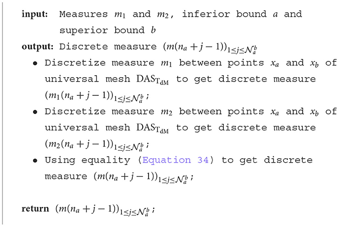
Algorithm 1. Computation discrete measure sum.

In what follows, the product measure is built for reasons of nature software production and to enrich the collection measure in the software tool. Figure 12 shows the resulting class diagram from the product measure. The tool is useful to display its data structure as methods and relationships and highlight process from this class. This measure is not used at the moment. In addition, some product operations are prohibited, as the product of two Dirac measures that have no sense in measure theory. The aim here is to express the product of two discrete measures and its integration. Thus, the product of two discrete measures ${(m_1(n_a+j-1))}_{1\le j\le {\mathcal{N}}_a^b}$ and ${(m_2(n_a+j-1))}_{1\le j\le {\mathcal{N}}_a^b}$ defined on the same universal mesh is discrete measure m(n_a+j−1) of ${\mathcal{N}}_a^b$ values given by,

$\begin{array}{ll}\forall j\in 〚1;{\mathcal{N}}_a^b〛,m(n_a+j-1)=\frac{m_1(n_a+j-1)\times m_2(n_a+j-1)}{T_{\text{dM}}}.& (35)\end{array}$

Figure 12

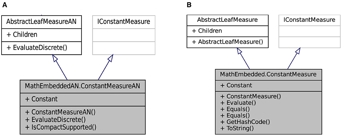
Figure 12. (A, B) Design, respectively, the class diagram of the product measure $\tilde{m}$ in low and high layers.

The integration of discrete measure ${(m(n_a+j-1))}_{1\le j\le {\mathcal{N}}_a^b}$ defined in relation (Equation 35) between inferior bound a and superior bound b is the sum of all values ${(m(n_a+j-1))}_{1\le j\le {\mathcal{N}}_a^b}$

$\begin{array}{ll}{\displaystyle \sum _{j=1}^{j={\mathcal{N}}_a^b}}m(n_a+j-1).& (36)\end{array}$

The consistency of relation (Equation 35) is illustrated by giving an example. This example consists in computing the discrete product of two discrete measures defined on the same universal mesh DAS_TdM. The first discrete measure ${(m_1(n_a+j-1))}_{1\le j\le {\mathcal{N}}_a^b}$ is defined by the discretization of constant measure with the constant C₁, between inferior bound x_a and superior bound x_b with discrete step T_dM,

$\begin{array}{ll}\forall j\in 〚1;{\mathcal{N}}_a^b〛,m_1(n_a+j-1)={\text{C}}_1\times T_{\text{dM}},& (37)\end{array}$

and the second discrete measure ${(m_2(n_a+j-1))}_{1\le j\le {\mathcal{N}}_a^b}$ is defined by the discretization of constant measure with the constant C₂, between inferior bound x_a and superior bound x_b with discrete step T_dM

$\begin{array}{ll}\forall j\in 〚1;{\mathcal{N}}_a^b〛,m_2(n_a+j-1)={\text{C}}_2\times T_{\text{dM}}.& (38)\end{array}$

Next, relation (Equation 35) is used for computing discrete product ${(m(n_a+j-1))}_{1\le j\le {\mathcal{N}}_a^b}$ to obtain:

$\begin{array}{ll}\forall j\in 〚1;{\mathcal{N}}_a^b〛,m(n_a+j-1)={\text{C}}_1\times {\text{C}}_2\times T_{\text{dM}}.& (39)\end{array}$

On the other hand, if the constant measure equals to C₁×C₂ is discretized between two points x_a and x_b of universal mesh DAS_TdM, then the same discrete value defined in relation (Equation 39) is obtained. Thus, the consistenty of the expression (Equation 35) is achieved. The integration of product measure at the high level is summarized in Algorithm 2.

Algorithm 2

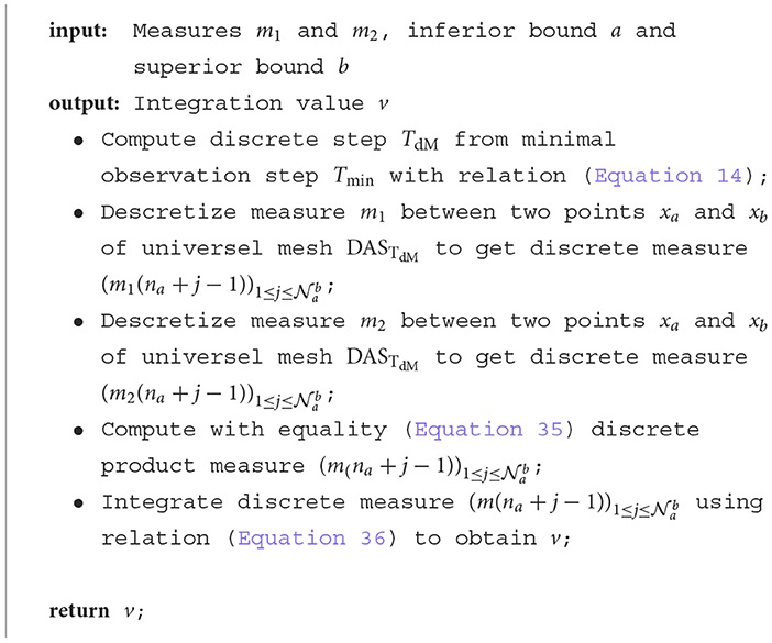
Algorithm 2. Integration algorithm of product m of two measures m₁ and m₂ in high level.

To reinforce the financial framework, a piecewise measure is defined by multiple sub-measuress, where each one applies to a different interval. The piecewise measure ${\tilde{m}}_{\mathrm{\text{Piecewise}}}$ that its class diagram shown in Figure 13 is one of the two construction methods defined from,

Figure 13

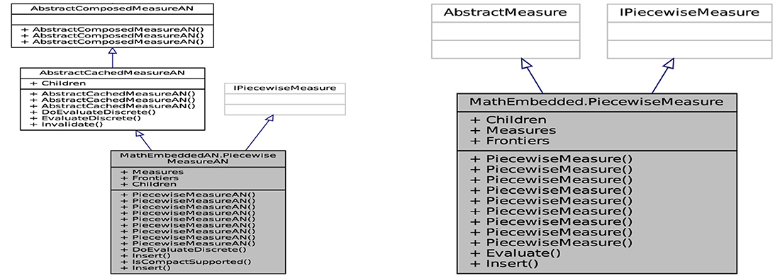
Figure 13. Class diagram of the piecewise measure ${\tilde{m}}_{\mathrm{\text{Piecewise}}}$ in two levels.

• a real Fr₀ allowing to generate measures m₀ and m₁, respectively, on intervals ]−∞, Fr₀] and [Fr₀, +∞[. Formally, measure ${\tilde{m}}_{\mathrm{\text{Piecewise}}}$ presented in Figure 14 is a piecewise measure on ℝ, if and only if,

$\exists F{r}_0\in ℝ,\text{ such that}:{\tilde{m}}_{\text{Piecewise}}{\mid }_{]-\infty ,F{r}_0]}=m_0,$

$\begin{array}{l}{\tilde{m}}_{\text{Piecewise}}{\mid }_{[F{r}_0,+\infty [}=m_1,\\ \text{where }{m}_0\text{and }{m}_1\text{ are any measures}.& (40)\end{array}$

Figure 14

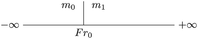
Figure 14. Piecewise measure ${\tilde{m}}_{\mathrm{\text{Piecewise}}}$ is composed of measures m₀, m₁, and frontier Fr₀.

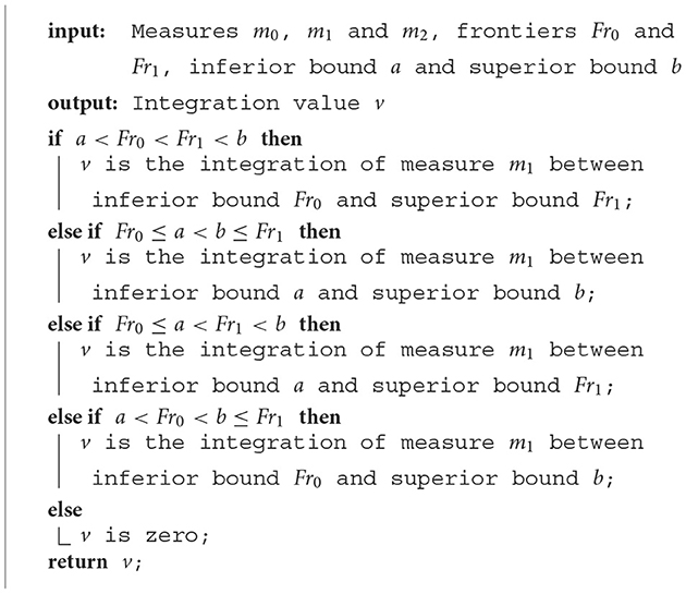
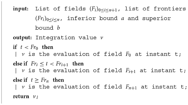
• a subdivision (Fr₀, Fr₁, …, Fr_n) of n+2 intervals allow to generate the measure m_i on each closed interval [Fr_i−1, Fr_i] for i from 1 to n and to generate both measures m₀ and m_n+1, respectively, on the two intervals ]−∞, Fr₀] and [Fr_n, +∞[. Formally, measure ${\tilde{m}}_{\mathrm{\text{Piecewise}}}$ presented in Figure 15 is a piecewise measure on ℝ, if and only if,

$\begin{array}{l}\exists (F{r}_0,F{r}_1,\dots ,F{r}_n),F{r}_0<F{r}_1<\dots <F{r}_n\text{such that}:\\ \forall i\in \{1,2,\dots ,n\}\\ {\tilde{m}}_{\text{Piecewise}}{\mid }_{]-\infty ,F{r}_0]}=m_0,{\tilde{m}}_{\text{Piecewise}}{\mid }_{[F{r}_{i-1},F{r}_i]}=m_i,\\ {\tilde{m}}_{\text{Piecewise}}{\mid }_{[F{r}_n,+\infty [}=m_{n+1},\\ \text{ where }{m}_0,m_i\text{ and }{m}_{n+1}\text{ are any measures}.& (41)\end{array}$

Figure 15

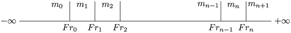
Figure 15. Piecewise measure ${\tilde{m}}_{\mathrm{\text{Piecewise}}}$ is composed with a list of measures (_{mi)0 ≤ i ≤ n+1} and of a list of frontiers (F_{ri)0 ≤ i ≤ n}.

Algorithm 3 depicts the integration of piecewise measure ${\tilde{m}}_{\mathrm{\text{Piecewise}}}$ defined in relation (Equation 40).

Algorithm 3

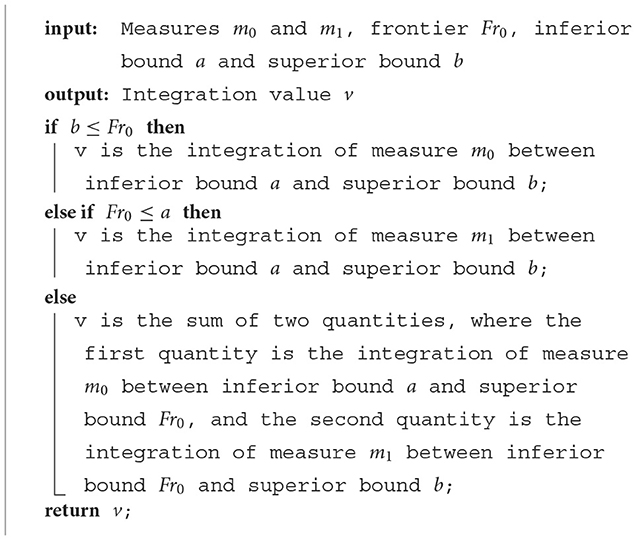
Algorithm 3. Integration algorithm of piecewise measure ${\tilde{m}}_{\mathrm{\text{Piecewise}}}$ defined in relation (Equation 40).

In order to integrate the piecewise measure ${\tilde{m}}_{\mathrm{\text{Piecewise}}}$ defined in relation (Equation 41) between inferior bound a and superior bound b, the index p and q are defined, respectively, by the indicators for first and last measures of (_{mi)0 ≤ i ≤ n+1} to be integrated. These index p et q are determined by dichotomy search. By considering l∈[[1;n]], index p, q∈[[0;n+1]] are defined using a list of frontiers (F_{ri)0 ≤ i ≤ n} as:

$\begin{array}{ll}p=\{\begin{array}{ll}0\hfill & \text{if }a<F{r}_0,\hfill \\ l\hfill & \text{if }F{r}_{l-1}\le a<F{r}_l,\hfill \\ n+1\hfill & \text{if }F{r}_n\le a.\hfill \end{array}& (42)\end{array}$

$\begin{array}{ll}q=\{\begin{array}{ll}0\hfill & \text{if }b\le F{r}_0,\hfill \\ l\hfill & \text{if }F{r}_{l-1}<b\le F{r}_l,\hfill \\ n+1\hfill & \text{if }F{r}_n<b.\hfill \end{array}& (43)\end{array}$

It is necessary to define variables a_⋆ and b_⋆ in order to integrate generally the piecewise measure ${\tilde{m}}_{\mathrm{\text{Piecewise}}}$. The variable a_⋆ means the superior integration bound of measure m_p. If a<Fr_n, then a_⋆ is equal to the inferior value of Fr_p and b, and if Fr_n ≤ a, then a_⋆ is equal to b. Formally, variable a_⋆ is defined as:

$\begin{array}{ll}{a}_{\star }=\{\begin{array}{ll}\inf \{F{r}_p,b\}\hfill & \text{if }a<F{r}_n,\hfill \\ b\hfill & \text{if }F{r}_n\le a.\hfill \end{array}& (44)\end{array}$

The variable b_⋆ signifies the inferior integration bound of measure m_q. Similary, if Fr₀<b, then b_⋆ is equal to the superior value of Fr_q−1 and of a, and if b ≤ Fr₀, then b_⋆ is equal to a. Formally, variable b_⋆ is defined as:

$\begin{array}{ll}{b}_{\star }=\{\begin{array}{ll}\sup \{F{r}_{q-1},a\}\hfill & \text{if }F{r}_0<b,\hfill \\ a\hfill & \text{if }b\le F{r}_0.\hfill \end{array}& (45)\end{array}$

Moreover, the quantities q₁, q₂, and q₃ are defined as follows. The quantity q₁ is the integration of measure m_p between inferior bound a and superior bound a_⋆,

$\begin{array}{ll}{q}_1={\displaystyle {\int }_a^{a_{\star }}}{m}_p.& (46)\end{array}$

The quantity q₂ is the sum of integration of measure m_i+1 between inferior bound Fr_i and superior bound Fr_i+1 for i from p to q−2:

$\begin{array}{ll}{q}_2={\displaystyle \sum _{i=p}^{i=q-2}}{\displaystyle {\int }_{F{r}_i}^{F{r}_{i+1}}}{m}_{i+1}.& (47)\end{array}$

The quantity q₃ is the integration of measure m_q between inferior bound b_⋆ and superior bound b:

$\begin{array}{ll}{q}_3={\displaystyle {\int }_{b_{\star }}^b}{m}_q.& (48)\end{array}$

Algorithm 4 incorporates the integration method of piecewise measure ${\tilde{m}}_{\mathrm{\text{Piecewise}}}$ defined in relation (Equation 41).

Algorithm 4

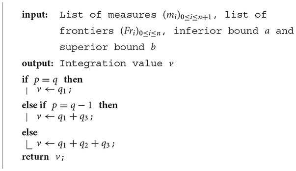
Algorithm 4. Integration algorithm of piecewise measure ${\tilde{m}}_{\mathrm{\text{Piecewise}}}$ defined in relation (Equation 41).

Another mathematical measure appended to the API is the truncated measure ${\tilde{m}}_{\mathrm{\text{Truncated}}}$. Figure 16 illustrates the ability to examine the entities and their relationships in the API from the truncated measure, which is one of the three construction methods defined from,

Figure 16

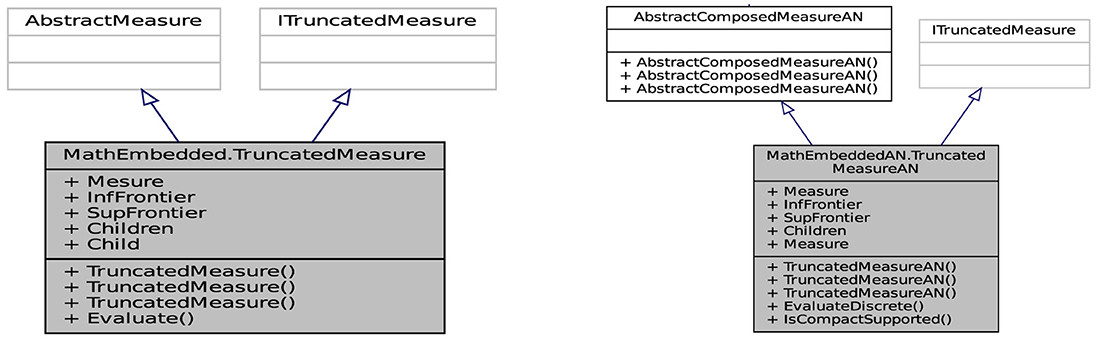
Figure 16. Class diagram of the truncated measure ${\tilde{m}}_{\mathrm{\text{Truncated}}}$.

• a subdivision (Fr₀, Fr₁) of three intervals allowing to generate the measure m₁ and null measures m₀ and m₂, respectively, on intervals [Fr₀, Fr₁] and ]−∞, Fr₀], [Fr₁, +∞[. Formally, measure ${\tilde{m}}_{\mathrm{\text{Truncated}}}$ shown in Figure 17 is a truncated measure on ℝ, if and only if,

$\begin{array}{l}\exists (F{r}_0,F{r}_1),F{r}_0<F{r}_1\\ \text{ s uch that}:{\tilde{m}}_{\text{Truncated}}{\mid }_{]-\infty ,F{r}_0]}=m_0,\\ {\tilde{m}}_{\text{Truncated}}{\mid }_{[F{r}_0,F{r}_1]}=m_1,\\ {\tilde{m}}_{\text{Truncated}}{\mid }_{[F{r}_1,+\infty [}=m_2,\text{where}\\ m_0,and{m}_2\\ \text{ are null measures and }{m}_1\text{is any measure}.& (49)\end{array}$

Figure 17

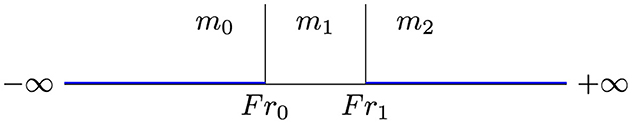
Figure 17. Truncated measure ${\tilde{m}}_{\mathrm{\text{Truncated}}}$ is composed of measure m₁, null measures m₀ and m₂, and frontiers Fr₀ and Fr₁.

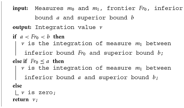
• a real Fr₀ allowing to generate the null measure m₀ and the measure m₁ on intervals ]−∞, Fr₀] and [Fr₀, +∞[, respectively. In other words, measure ${\tilde{m}}_{\mathrm{\text{Truncated}}}$ illustrated in Figure 18 is a truncated measure on ℝ, if and only if,

$\begin{array}{l}\exists F{r}_0\in ℝ,\text{such that}:{\tilde{m}}_{\text{Truncated}}{\mid }_{]-\infty ,F{r}_0]}=m_0,\\ {\tilde{m}}_{\text{Truncated}}{\mid }_{[F{r}_0,+\infty [}=m_1,\\ \text{ where }{m}_0\text{is null measure and }{m}_1\text{is any measure}.& (50)\end{array}$

Figure 18

Figure 18. Truncated measure ${\tilde{m}}_{\mathrm{\text{Truncated}}}$ is composed of null measure m₀, measure m₁, and frontier Fr₀.

• a real Fr₁ allowing to generate the measures m₁ and m₂ on intervals ]−∞, Fr₁] and [Fr₁, +∞[, respectively. In other words, measure ${\tilde{m}}_{\mathrm{\text{Truncated}}}$ presented in Figure 19 is a truncated measure on ℝ, if and only if,

$\begin{array}{l}\exists F{r}_1\in ℝ\text{ such that}:{\tilde{m}}_{\text{Truncated}}{\mid }_{]-\infty ,F{r}_1]}=m_1,\\ {\tilde{m}}_{\text{Truncated}}{\mid }_{[F{r}_1,+\infty [}=m_2,\\ \text{ where }{m}_1\text{ is any measure and }{m}_2\text{ is null measure}.& (51)\end{array}$

Figure 19

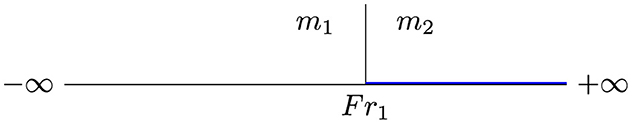
Figure 19. Truncated measure ${\tilde{m}}_{\mathrm{\text{Truncated}}}$ is composed of measure m₁, null measure m₂, and frontier Fr₁.

Note that the truncated measure ${\tilde{m}}_{\mathrm{\text{Truncated}}}$ is created for instance to calculate the amount borrowed over a time interval from a truncated and restricted loan over time intervals. Algorithms 5–7 illustrate the integration of this measure defined, respectively, in relations (Equations 48, 49) between inferior bound a and superior bound b.

Algorithm 5

Algorithm 5. Integration algorithm of truncated measure ${\tilde{m}}_{\mathrm{\text{Truncated}}}$ defined in relation (Equation 49).

Algorithm 6

Algorithm 6. Integration algorithm of truncated measure ${\tilde{m}}_{\mathrm{\text{Truncated}}}$ defined in relation (Equation 50).

Algorithm 7

Algorithm 7. Integration algorithm of truncated measure ${\tilde{m}}_{\mathrm{\text{Truncated}}}$ defined in relation (Equation 51).

The tabulated measure is created for three reasons. The first one is to translate an array of values into a discrete measure. The second one is to compute the convolution measure. Finally, the last one is to generate a discrete measure in low level to transfer it to the high level. The aim is to build a tabulated measure ${\tilde{m}}_{\mathrm{\text{Tabulated}}}$ between inferior value V_I and superior bound V_S strictly superior than V_I with a set of n values (_{li)0 ≤ i ≤ n−1}. A tabulation step T_tab is used to share values (_{li)0 ≤ i ≤ n−1} between V_I and V_S, defined by:

$\begin{array}{ll}{T}_{\text{tab}}=\frac{V_S-V_I}{n}.& (52)\end{array}$

The tabulated measure ${\tilde{m}}_{\mathrm{\text{Tabulated}}}$ is a construction method defined from a subdivision (Fr₀, Fr₁, …, Fr_n) given by following frontiers:

$\begin{array}{l}\forall i\in 〚0;n〛,F{r}_i=V_I+i\times T_{\text{tab}},\end{array}$

permitting to generate the constant density m_j+1 on each closed interval [Fr_j, Fr_j+1] for j from 0 to n−1, and to generate both null densities m₀ and m_n+1, respectively, on intervals ]−∞, Fr₀] and [Fr_n, +∞[.

To integrate the tabulated measure ${\tilde{m}}_{\mathrm{\text{Tabulated}}}$ explicitly between inferior bound a and superior bound b, index p and q given, respectively, in relations (Equations 41, 42) are used. Indeed, the measure ${\tilde{m}}_{\mathrm{\text{Tabulated}}}$ is constituted with null densities m₀ and m_n+1. Algorithm 8 summarizes its implementation.

Algorithm 8

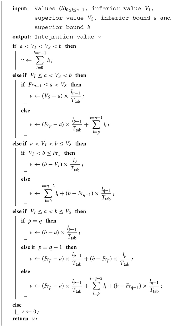
Algorithm 8. Integration algorithm of tabulated measure ${\tilde{m}}_{\mathrm{\text{Tabulated}}}$.

The discrete convolution is a fundamental operation in the financial model. It is imperative to implement it in order to compute repayment amount with the aid of the Fast Fourier Transform (FFT) method. We refer to articles (Liang et al., 2019; Zlateski et al., 2019) which deal with how FFT can efficiently compute convolution. An algorithm based on convolution theorem stated in Zlateski et al. (2019) was performed using Fourier transforms with much fewer operations. Article Liang et al. (2019) designs its efficient computation with highly optimized FFT implementation.

We have investigated two approaches to compute the discrete convolution. Assuming certain regularity on the proposal measures ${\tilde{\kappa }}_E$ and ${\tilde{\rho }}_{\mathcal{K}}$. The first approach consists of applying directly the Fourier convolution operator ℱ and its inverse to equality (Equation 5) without change of coordinates, which becomes,

$\begin{array}{l}{\tilde{\rho }}_{\mathcal{K}}={\mathcal{F}}^{-1}(\mathcal{F}({\tilde{\kappa }}_E)•\mathcal{F}(\tilde{\gamma })).\end{array}$

The objective of the second approach is to express the convolution product defined in Equation 5 in term of convolution product of two functions defined on the interval [0, 1]. Assuming that the convex hull of the supported measures ${\tilde{\kappa }}_E$ and $\tilde{\gamma }$ are, respectively, intervals [a, b] and [c, d], as presented in Figure 20. Then, the predicted convex hull generated by the class convolution ${\tilde{\kappa }}_E\star \tilde{\gamma }$ is a closed interval contained in [a+c, b+d]. This is read as,

$\begin{array}{l}\text{CV}({\tilde{\kappa }}_E)=\left[a,b\right],\text{CV}(\tilde{\gamma })=\left[c,d\right]\Rightarrow \text{CV}({\tilde{\kappa }}_E\star \tilde{\gamma })\subset \left[a+c,b+d\right].\end{array}$

Figure 20

Figure 20. Convolution of two Gaussian distributions with variable shift to interval [0, 1].

Defining the function ${\kappa }_E^T$ by the translated function of κ_E, that is, ${\kappa }_E^T(y)={\kappa }_E(y-c+a)$, then, the convex hull of the density ${\kappa }_E^T$ is the interval [c, e], where e = c+(b−a). By making the following change of variable Y = y+c−a, we will obtain,

$\begin{array}{l}{\kappa }_E\star \gamma (x)={\kappa }_E^T\star \gamma (x+c-a).\end{array}$

Defining the functions ${{\kappa }_E}^{0,1}$ and γ^{0, 1} by the respective contracted functions of ${\kappa }_E^T$ and γ on the interval [0, 1]

$\begin{array}{ll}{{\kappa }_E}^{0,1}(x)={\kappa }_E^T((max(e,d)-c)x+c),{\gamma }^{0,1}(x)=\gamma ((max(e,d)-c)x+c).& (53)\end{array}$

Next, making the following change of variable $z=\frac{y-c}{max(e,d)-c}$ in the integral operator, we can prove that,

$\begin{array}{l}{\kappa }_E\star \gamma (x)=(max(e,d)-c)\times {{\kappa }_E}^{0,1}\star {\gamma }^{0,1}\left(\frac{x-c-a}{max(e,d)-c}\right).\end{array}$

The first approach does not require a change of coordinates. Exploring the second approach remains interesting. A study investigating the comparison of the time computation between these two approaches demonstrated that the first approach is more efficient than the second one. Determining the convex hull of the support from discrete measures is a necessary step in the computed convolution. The next step is to complete these discrete measures by zero such that they have N smallest values, where N is a power of two. Then, the computed vector defined by element-wise multiplication is also requested. Finally, constructing the tabulated measure from this vector and discretizing it is crucial in evaluating the repayment amount.

The field is defined as a continuous function by superior value. Fields are shared in two categories which are simple and composed. The purpose is to provide them definitions and how they are evaluated in high level at point. The discretization of non-discrete fields in low level is based on the evaluation. A simple field can be constant, affine, quadratic, polynomial, exponential, etc. For instance, the constant field is created in order to compute the borrowed amount at a given instant where the loan is a constant function. The constant field F_Constant is defined as the function that is equal to C independently of variable time t,

$\begin{array}{ll}\forall t\in ℝ,F_{\text{Constant}}(t)=\text{C}.& (54)\end{array}$

The evaluation of the constant field F_Constant given by Equation 53 returns constant C. The table in Appendix B summarizes the evaluation of some simple fields. A composed field can be sum, product, piecewise, truncated, or other. The sum field is built to compute the sum of two fields at the instant t. The evaluation of the sum F of two fields F₁ and F₂ in high level at instant t returns a value which is the sum of two values. The first value is the evaluation of field F₁ at time t, and the second value is the evaluation of field F₂ at time t. By the same way the product F of two fields is implemented. They are defined as,

$\begin{array}{ll}\forall t\in ℝ,\text{F}(t)={\text{F}}_1(t)+{\text{F}}_2(t),\text{F}(t)={\text{F}}_1(t)\times {\text{F}}_2(t).& (55)\end{array}$

Algorithm 9 is designed for evaluating piecewise field F_Piecewise, defined from a real Fr₀ allowing to generate fields F₀ and F₁, respectively, on intervals ]−∞, Fr₀] and [Fr₀, +∞[. The field F_Piecewise is a piecewise field on ℝ, if and only if,

$\begin{array}{l}\exists F{r}_0\in ℝ,\text{ such that}:\\ {\text{F}}_{\text{Piecewise}}{\mid }_{]-\infty ,F{r}_0]}=F_0,\\ {\text{F}}_{\text{Piecewise}}{\mid }_{[F{r}_0,+\infty [}=F_1,\\ \text{ where }{F}_0\text{ and}\\ F_1\text{ are any fields}.& (56)\end{array}$

Algorithm 9

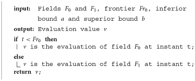
Algorithm 9. Evaluation algorithm of piecewise field F_Piecewise defined in relation (Equation 54).

Algorithm 10 illustrates the evaluation of piecewise field F_Piecewise, determined from a subdivision (Fr₀, Fr₁, …, Fr_n) of n+2 intervals allowing to generate the field F_i on each closed interval [Fr_i−1, Fr_i] for i from 1 to n and to generate both fields F₀ and F_n+1, respectively, on two intervals ]−∞, Fr₀] and [Fr_n, +∞[. The field F_Piecewise is a piecewise field on ℝ, if and only if,

$\begin{array}{l}\exists (F{r}_0,F{r}_1,\dots ,F{r}_n),,F{r}_0<F{r}_1<\dots <F{r}_n\\ \text{ such that}:\forall i\in \{1,2,\dots ,n\}\\ {\text{F}}_{\text{Piecewise}}{\mid }_{[F{r}_{i-1},F{r}_i]}=F_i,{\text{F}}_{\text{Piecewise}}\end{array}$

$\begin{array}{l}{\mid }_{]-\infty ,F{r}_0]}=F_0,{\text{F}}_{\text{Piecewise}}{\mid }_{[F{r}_n,+\infty [}=F_{n+1},\\ \text{ where }{F}_i,F_0,F_{n+1}\text{ are any fields}.\end{array}$

Algorithm 10

Algorithm 10. Evaluation algorithm of piecewise field F_Piecewise defined in relation (Equation 54).

Assuming that truncated field F_Truncated is a construction method defined from a subdivision (Fr₀, Fr₁) of 3 intervals allowing to generate the field F₁ on interval [Fr₀, Fr₁] and to generate both null fields F₀ and F₂, respectively, on intervals ]−∞, Fr₀] and [Fr₁, +∞[. Formally, field F_Truncated is a truncated field on ℝ, if and only if,

$\begin{array}{l}\exists (F{r}_0,F{r}_1),F{r}_0<F{r}_1\\ \text{ such that}:{\text{F}}_{\text{Truncated}}{\mid }_{]-\infty ,F{r}_0]}=F_0,\\ {\text{F}}_{\text{Truncated}}{\mid }_{[F{r}_0,F{r}_1]}=F_1,\\ {\text{F}}_{\text{Truncated}}{\mid }_{[F{r}_1,+\infty [}=F_2,\text{where}\\ F_0\text{ and }{F}_2\text{ are null fields and }{F}_1\text{ is any field}.& (57)\end{array}$

Then, Algorithm 11 depicts the evaluation of truncated field F_Truncated given by Equation 54 at instant t.

Algorithm 11

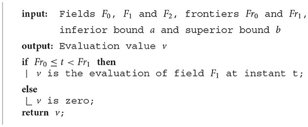
Algorithm 11. Evaluation algorithm of truncated field F_Truncated defined in relation (Equation 57).

The purpose here is to present the fast implementation of quadtratic interpolation operator for field F_d that is improved than the linear one. Piecewise-linear functions (Zhang et al., 2021; Goujon et al., 2023) have been used to estimate one-dimensional functions for generations. Then, the restriction of the field F_d is determined at each period interval [y_k, y_k+2[ with three key-value pairs. The field interpolates the values $F_d^{\mathrm{\text{D}}}(n_a+k-1)$, $F_d^{\mathrm{\text{D}}}(n_a+k)$, and $F_d^{\mathrm{\text{D}}}(n_a+k+1)$ in, respectively, points y_k, y_k+1, and y_k+2 for each integer $k\in 〚1;{\mathcal{N}}_a^b〛$. The set of points y_k follows the definition Equation 10 even for fields. The discrete step T_dF defined for fields plays the same rule of discrete step T_dM for measures. Formally, the field F_d can be written in the following quadratic formula,

$\forall k\in [\text{}[1;{\mathcal{N}}_a^b]\text{}],\forall t\in [y_k,y_{k+2}[,F_d(t)=\zeta t^2+\alpha t+\beta .$

In which unknown variables ζ, α, and β are necessary to be determined in terms of discrete step T_dF and values ${(F_d^{\mathrm{\text{D}}}(n_a+k-1))}_{1\le k\le {\mathcal{N}}_a^b+1}$. This involves establishing the following system,

$\begin{array}{ll}\forall k\in [\text{}[1;{\mathcal{N}}_a^b]\text{}],\{\begin{array}{l}\zeta y_k^2+\alpha y_k+\beta =F_d^{\text{D}}(n_a+k-1),\hfill \\ \zeta y_{k+1}^2+\alpha y_{k+1}+\beta =F_d^{\text{D}}(n_a+k),\hfill \\ \zeta y_{k+2}^2+\alpha y_{k+2}+\beta =F_d^{\text{D}}(n_a+k+1).\hfill \end{array}& (58)\end{array}$

The equation system given by Equation 55 is reduced to double equations to allow expressing the growth rates $F_d^{\mathrm{\text{D}}}(n_a+k+1)-F_d^{\mathrm{\text{D}}}(n_a+k)$ and $F_d^{\mathrm{\text{D}}}(n_a+k)-F_d^{\mathrm{\text{D}}}(n_a+k-1)$ in terms of coefficients ζ and α. Formally, the coefficient ζ is determined as,

$\begin{array}{ll}\zeta =\frac{F_d^{\text{D}}(n_a+k+1)-2F_d^{\text{D}}(n_a+k)+F_d^{\text{D}}(n_a+k-1)}{2T_{\text{dF}}^2}.& (59)\end{array}$

Since ζ is determined by equality (Equation 56), the growth rate $F_d^{\mathrm{\text{D}}}(n_a+k)-F_d^{\mathrm{\text{D}}}(n_a+k-1)$ permits to find out the coefficient α with the following expression,

$\begin{array}{l}\alpha =\frac{F_d^{\text{D}}(n_a+k)-F_d^{\text{D}}(n_a+k-1)}{T_{\text{dF}}}-(2y_k+T_{\text{dF}})\\ \times \left(\frac{F_d^{\text{D}}(n_a+k+1)-2F_d^{\text{D}}(n_a+k)+F_d^{\text{D}}(n_a+k-1)}{2T_{\text{dF}}^2}\right).& (60)\end{array}$

Finally, to achieve the definition of the field F_d, the estimated coefficient β is obtained by,

$\begin{array}{l}\beta =F_d^{\text{D}}(n_a+k-1)-\frac{F_d^{\text{D}}(n_a+k)-F_d^{\text{D}}(n_a+k-1)}{T_{\text{dF}}}\\ +(y_k^2+y_k{T}_{\text{dF}})\\ \times \left(\frac{F_d^{\text{D}}(n_a+k+1)-2F_d^{\text{D}}(n_a+k)+F_d^{\text{D}}(n_a+k-1)}{2T_{\text{dF}}^2}\right).\end{array}$

After giving a brief detail about evaluating a field, we recall that the Current Debt Field 𝒦_RD is related to Loan Measure ${\tilde{\kappa }}_E$ and Repayment Measure ${\tilde{\rho }}_{\mathcal{K}}$ by the following partial equation:

$\begin{array}{ll}\frac{d{\mathcal{K}}_{RD}}{dt}={\kappa }_E(t)-{\rho }_{\mathcal{K}}(t)-{\rho }_{\mathcal{K}}^{\text{I}}(t).& (61)\end{array}$

In which Repayment Measure ${\tilde{\rho }}_{\mathcal{K}}$ is defined by Equation 5, and measure ${\tilde{\rho }}_{\mathcal{K}}^{\mathtt{\text{I}}}$ associated with density ${\rho }_{\mathcal{K}}^{\mathtt{\text{I}}}$ is the Initial Debt Repayment Plan and expresses how current debt amount at the initial time will be repaid. The solution of this ODE (Ordinary Differential Equation) is expressed as,

$\begin{array}{ll}{\mathcal{K}}_{RD}(t)={\mathcal{K}}_{RD}(t_{\text{I}})+{\displaystyle {\int }_{t_{\text{I}}}^t}{\tilde{\kappa }}_E-{\displaystyle {\int }_{t_{\text{I}}}^t}{\tilde{\rho }}_{\mathcal{K}}-{\displaystyle {\int }_{t_{\text{I}}}^t}{\tilde{\rho }}_{\mathcal{K}}^{\text{I}}.& (62)\end{array}$

To evaluate the field 𝒦_RD given by Equation 59 at an instant t, a new method intends to compute the primitive of a measure is implemented. This method is based on numerical approach contained in accumulating a discrete measure to approximate it by a piecewise function. Note that a primitive of measure m_d in low level, null at point x_c is a field F_d. The classical discretization of this object field F_d is defined by discrete field ${(F_d^{\mathrm{\text{D}}}(n_a+k-1))}_{1\le k\le {\mathcal{N}}_a^b+1}$ given by,

$\begin{array}{ll}\forall k\in 〚1;{\mathcal{N}}_a^b+1〛,F_d^{\text{D}}(n_a+k-1)={\displaystyle {\int }_{x_c}^{y_k}}{m}_d.& (63)\end{array}$

Three situations can be distinguished (x_c<x_a, x_b<x_c, x_a ≤ x_c ≤ x_b) to compute the discrete field ${(F_d^{\mathrm{\text{D}}}(n_a+k-1))}_{1\le k\le {\mathcal{N}}_a^b+1}$. In all these cases, the discrete field given by equality (Equation 60) can be written as a summation of discrete measure using Chasles relation.

7 Conclusion and future work

This study presents a comprehensive survey in which measure theory is applied to financial modeling. This theory is needed, in an essential way, to transform the discrete-time framework into the continuous one. In practice, to use the standard tools of this theory, some technical developments based on modern software architecture are imposed. In passing, it is not easy to integrate some fields with respect to some measures to evaluate a variety of capital, investment, and trade received by the organizations. Another aspect of this problem is that conceiving and implementing algorithms in the dual vector space of continuous piecewise function is not suitable. Within the continuous-in-time financial framework, there was a unique API for interacting with the SOFI solver. Making some numerical choices in this space makes sure that the operations between measures and fields will be ensured.

Our purpose was to produce a financial library enabling us to test our ideas and some actions to be maintained. The library should then be simply extendible with respect to frameworks with variable rates set at instants of borrowing or with varying Repayment Patterns. Particularly, high-level interfaces modeling the layers are designed to manage the complex data structures requested by the library components. Further to the implementation, we have created test projects to review implementation results and cover a significant proportion of the code. The layered architecture design allows the implementation of the new functional requirement sets needed for the measure theory paradigm. Another important criterion in the design of the API is consistency. This consistency has proven that at least 96% of errors are not violated of constraints on classes and objects. This performance penalty is taken into account for production computations. Developing a commercial C# that fits the quality requirements achieves a high maintainability API. The implemented framework considers the defined time period of interest only once before setting out the budget project. However, the discrete model has drawbacks in managing it during this period.

We have investigated one preferred way to write multithreaded and parallel API using modern asynchronous methods built on Task. The foundation for our parallelism is based on the TPL library. The future work of this research includes making the parallel API faster and more scalable. It is essential to use parallel abstractions well when distributing the tasks between the available threads. Treating Tasks at a low level and migrating values to a high level is done by a performed mechanism tool, but it requires much analysis and optimization procedures. The data parallelism should be controlled by performing various operations between tasks. For instance, logical task patterns should also be separated from physical threads into hierarch data structures. Another challenge is facilitating locality and parallelism of tasks during intensive computations.

Data availability statement

The original contributions presented in the study are included in the article/Supplementary material, further inquiries can be directed to the corresponding author.

Author contributions

TC: Writing – original draft, Writing – review & editing.

Funding

The author(s) declare financial support was received for the research, authorship, and/or publication of this article. This study was jointly funded by MGDIS Company (http://www.mgdis.fr/) and the LMBA (http://www.lmba-math.fr/). The funders were not involved in the study design, collection, analysis, interpretation of data.

Acknowledgments

The author address many thanks to the reviewers for their helpful and valuable comments that have greatly improved the study.

Conflict of interest

The author declares that the research was conducted in the absence of any commercial or financial relationships that could be construed as a potential conflict of interest.

Publisher's note

All claims expressed in this article are solely those of the authors and do not necessarily represent those of their affiliated organizations, or those of the publisher, the editors and the reviewers. Any product that may be evaluated in this article, or claim that may be made by its manufacturer, is not guaranteed or endorsed by the publisher.

Supplementary material

The Supplementary Material for this article can be found online at: https://www.frontiersin.org/articles/10.3389/fcomp.2024.1371052/full#supplementary-material

References

Alshamrani, R., Alshehri, F., and Kurdi, H. (2020). A preprocessing technique for fast convex hull computation. Procedia Comput. Sci. 170, 317–324. doi: 10.1016/j.procs.2020.03.046

Crossref Full Text | Google Scholar

Andreev, A. V., Maksimenko, V. A., Pisarchik, A. N., and Hramov, A. E. (2021). Synchronization of interacted spiking neuronal networks with inhibitory coupling. Chaos, Solitons Fract. 146:110812. doi: 10.1016/j.chaos.2021.110812

Crossref Full Text | Google Scholar

Bossen, F., Sühring, K., Wieckowski, A., and Liu, S. (2021). VVC complexity and software implementation analysis. IEEE Trans. Circ. Syst. Video Technol. 31, 3765–3778. doi: 10.1109/TCSVT.2021.3072204

Crossref Full Text | Google Scholar

Chakkour, T. (2017a). Implementing some mathematical operators for a continuous-in-time financial model. Eng. Math. Lett. 2017:2.

Google Scholar

Chakkour, T. (2017b). Some notes about the continuous-in-time financial model. Abstr. Appl. Anal. 2017:6985820. doi: 10.1155/2017/6985820

Crossref Full Text | Google Scholar

Chakkour, T. (2019). Inverse problem stability of a continuous-in-time financial model. Acta Mathem. Scient. 39, 1423–1439. doi: 10.1007/s10473-019-0519-5

Crossref Full Text | Google Scholar

Chakkour, T. (2022). “Numerical simulation of pipes with an abrupt contraction using openfoam,” in Fluid Mechanics at Interfaces 2: Case Studies and Instabilities, 45–75. doi: 10.1002/9781119903000.ch3

Crossref Full Text | Google Scholar

Chakkour, T. (2023). Some inverse problem remarks of a continuous-in-time financial model in l 1 ([ti, θ max]). Mathem. Model. Comput. 10, 864–874. doi: 10.23939/mmc2023.03.864

Crossref Full Text | Google Scholar

Chakkour, T. (2024a). Finite element modelling of complex 3d image data with quantification and analysis. Oxford Open Materials Sci. 4:itae003. doi: 10.1093/oxfmat/itae003

PubMed Abstract | Crossref Full Text | Google Scholar

Chakkour, T. (2024b). Parallel computation to bidimensional heat equation using MPI/cuda and fftw package. Front. Comput. Sci. 5:1305800. doi: 10.3389/fcomp.2023.1305800

Crossref Full Text | Google Scholar

Chakkour, T., and Frénod, E. (2016). Inverse problem and concentration method of a continuous-in-time financial model. Int. J. Finan. Eng. 3:1650016. doi: 10.1142/S242478631650016X

Crossref Full Text | Google Scholar

Chen, X., Huang, F., and Li, X. (2022). Robust asset-liability management under CRRA utility criterion with regime switching: a continuous-time model. Stochastic Models 38, 167–189. doi: 10.1080/15326349.2021.1985520

Crossref Full Text | Google Scholar

Cheng, J., Chen, Q., and Huang, X. (2023). An algorithm for crack detection, segmentation, and fractal dimension estimation in low-light environments by fusing FFT and convolutional neural network. Fractal Fract. 7:820. doi: 10.3390/fractalfract7110820

Crossref Full Text | Google Scholar

Chung, J., and Lee, J. M. (1994). A new family of explicit time integration methods for linear and non-linear structural dynamics. Int. J. Numer. Methods Eng. 37, 3961–3976. doi: 10.1002/nme.1620372303

Crossref Full Text | Google Scholar

Cywiak, M., and Cywiak, D. (2021). “Sympy,” in Multi-Platform Graphics Programming with Kivy: Basic Analytical Programming for 2D, 3D, and Stereoscopic Design (Springer), 173–190. doi: 10.1007/978-1-4842-7113-1_11

Crossref Full Text | Google Scholar

Dolgov, S., Kalise, D., and Saluzzi, L. (2023). Data-driven tensor train gradient cross approximation for hamilton-jacobi-bellman equations. SIAM J. Sci. Comput. 45, A2153–A2184. doi: 10.1137/22M1498401

Crossref Full Text | Google Scholar

Dumka, P., Dumka, R., and Mishra, D. R. (2022). Numerical Methods using Python (For scientists and Engineers). London: Blue Rose Publishers.

Google Scholar

Eling, M., and Loperfido, N. (2020). New mathematical and statistical methods for actuarial science and finance. Eur. J. Finance 26, 96–99. doi: 10.1080/1351847X.2019.1707251

Crossref Full Text | Google Scholar

Fang, F., Ventre, C., Basios, M., Kanthan, L., Martinez-Rego, D., Wu, F., et al. (2022). Cryptocurrency trading: a comprehensive survey. Finan. Innov. 8, 1–59. doi: 10.1186/s40854-021-00321-6

PubMed Abstract | Crossref Full Text | Google Scholar

Farimani, S. A., Jahan, M. V., Fard, A. M., and Tabbakh, S. R. K. (2022). Investigating the informativeness of technical indicators and news sentiment in financial market price prediction. Knowl. Based Syst. 247:108742. doi: 10.1016/j.knosys.2022.108742

Crossref Full Text | Google Scholar

Frénod, E., and Chakkour, T. (2016). A continuous-in-time financial model. Mathem. Finance Lett. 2016, 1–36.

Google Scholar

Gao, X., Saha, R. K., Prasad, M. R., and Roychoudhury, A. (2020). “Fuzz testing based data augmentation to improve robustness of deep neural networks,” in Proceedings of the ACM/IEEE 42nd International Conference on Software Engineering, 1147–1158. doi: 10.1145/3377811.3380415

Crossref Full Text | Google Scholar

Gaston, D., Newman, C., Hansen, G., and Lebrun-Grandie, D. (2009). Moose: a parallel computational framework for coupled systems of nonlinear equations. Nuclear Eng. Des. 239, 1768–1778. doi: 10.1016/j.nucengdes.2009.05.021

Crossref Full Text | Google Scholar

Gilli, M., Maringer, D., and Schumann, E. (2019). Numerical Methods and Optimization in Finance. New York: Academic Press. doi: 10.1016/B978-0-12-815065-8.00022-4

Crossref Full Text | Google Scholar

Golmohammadi, A., Zhang, M., and Arcuri, A. (2023). .net/c# instrumentation for search-based software testing. Softw. Quality J. 31, 1439–1465. doi: 10.1007/s11219-023-09645-1

Crossref Full Text | Google Scholar

Górski, T. (2022). Reconfigurable smart contracts for renewable energy exchange with re-use of verification rules. Appl. Sci. 12:5339. doi: 10.3390/app12115339

Crossref Full Text | Google Scholar

Goujon, A., Campos, J., and Unser, M. (2023). Stable parameterization of continuous and piecewise-linear functions. Appl. Comput. Harmon. Anal. 67:101581. doi: 10.1016/j.acha.2023.101581

Crossref Full Text | Google Scholar

Guo, Z., Huang, T.-W., and Lin, Y. (2023). “Accelerating static timing analysis using CPU-GPU heterogeneous parallelism,” in IEEE Transactions on Computer-Aided Design of Integrated Circuits and Systems, 4973–4984. doi: 10.1109/TCAD.2023.3286261

Crossref Full Text | Google Scholar

Guseinov, G. S. (2003). Integration on time scales. J. Math. Anal. Appl. 285, 107–127. doi: 10.1016/S0022-247X(03)00361-5

Crossref Full Text | Google Scholar

Hahn, T. (2005). Cuba-a library for multidimensional numerical integration. Comput. Phys. Commun. 168, 78–95. doi: 10.1016/j.cpc.2005.01.010

Crossref Full Text | Google Scholar

Hickey, L., and Harrigan, M. (2022). The BISQ decentralised exchange: on the privacy cost of participation. Blockchain 3:100029. doi: 10.1016/j.bcra.2021.100029

Crossref Full Text | Google Scholar

Huang, T.-W., Lin, D.-L., Lin, C.-X., and Lin, Y. (2021). “Taskflow: a lightweight parallel and heterogeneous task graph computing system,” in IEEE Transactions on Parallel and Distributed Systems, 1303–1320. doi: 10.1109/TPDS.2021.3104255

Crossref Full Text | Google Scholar

Hung, M.-C., Chen, A.-P., and Yu, W.-T. (2024). AI-driven intraday trading: applying machine learning and market activity for enhanced decision support in financial markets. IEEE Access. 12, 12953–12962. doi: 10.1109/ACCESS.2024.3355446

Crossref Full Text | Google Scholar

Kang, M., Lee, E. T., Um, S., and Kwak, D.-H. (2023). Development of a method framework to predict network structure dynamics in digital platforms: empirical experiments based on API networks. Knowl.-Based Syst. 280:110936. doi: 10.1016/j.knosys.2023.110936

Crossref Full Text | Google Scholar

Kao, E. P. (2019). An Introduction to Stochastic Processes. New York: Courier Dover Publications.

Google Scholar

Keith, A., Ferrada, H., and Navarro, C. A. (2022). “Accelerating the convex hull computation with a parallel GPU algorithm,” in 2022 41st International Conference of the Chilean Computer Science Society (SCCC) (IEEE), 1–7. doi: 10.1109/SCCC57464.2022.10000307

Crossref Full Text | Google Scholar

Knueven, B., Ostrowski, J., Castillo, A., and Watson, J.-P. (2022). A computationally efficient algorithm for computing convex hull prices. Comput. Ind. Eng. 163:107806. doi: 10.1016/j.cie.2021.107806

PubMed Abstract | Crossref Full Text | Google Scholar

Kundu, S., and Makri, N. (2023). Pathsum: a c++ and fortran suite of fully quantum mechanical real-time path integral methods for (multi-) system+ bath dynamics. J. Chem. Phys. 158:481. doi: 10.1063/5.0151748

PubMed Abstract | Crossref Full Text | Google Scholar

Leijen, D., Schulte, W., and Burckhardt, S. (2009). The design of a task parallel library. ACM Sigplan Notices 44, 227–242. doi: 10.1145/1639949.1640106

Crossref Full Text | Google Scholar

Li, C., Cheng, Z., Zhu, H., Wang, L., Lv, Q., Wang, Y., et al. (2022). Dmalnet: dynamic malware analysis based on API feature engineering and graph learning. Comput. Secur. 122:102872. doi: 10.1016/j.cose.2022.102872

Crossref Full Text | Google Scholar

Liang, Y., Lu, L., Xiao, Q., and Yan, S. (2019). Evaluating fast algorithms for convolutional neural networks on FPGAs. IEEE Trans. Comput.-Aided Des. Integr. Circ. Syst. 39, 857–870. doi: 10.1109/TCAD.2019.2897701

Crossref Full Text | Google Scholar

Lima, J. A. P., and Vergilio, S. R. (2020). Test case prioritization in continuous integration environments: a systematic mapping study. Inf. Softw. Technol. 121:106268. doi: 10.1016/j.infsof.2020.106268

Crossref Full Text | Google Scholar

Lin, C.-X., Huang, T.-W., and Wong, M. D. (2020). “An efficient work-stealing scheduler for task dependency graph,” in 2020 IEEE 26th International Conference on Parallel and Distributed Systems (ICPADS) (IEEE), 64–71. doi: 10.1109/ICPADS51040.2020.00018

Crossref Full Text | Google Scholar

Liu, C., Li, B., Zhao, J., Zhen, Z., Feng, W., and Liu, X. (2023). TI-MVD: a temporal interaction-enhanced model for malware variants detection. Knowl. Based Syst. 278:110850. doi: 10.1016/j.knosys.2023.110850

Crossref Full Text | Google Scholar

Liu, Z., Hu, X., Xu, L., Wang, W., and Ghannouchi, F. M. (2021). Low computational complexity digital predistortion based on convolutional neural network for wideband power amplifiers. IEEE Trans. Circ. Syst. Expr. Briefs 69, 1702–1706. doi: 10.1109/TCSII.2021.3109973

Crossref Full Text | Google Scholar

Machné, R., Finney, A., Müller, S., Lu, J., Widder, S., and Flamm, C. (2006). The SBML ode solver library: a native API for symbolic and fast numerical analysis of reaction networks. Bioinformatics 22, 1406–1407. doi: 10.1093/bioinformatics/btl086

PubMed Abstract | Crossref Full Text | Google Scholar

Marin, G., and Vona, F. (2023). Finance and the reallocation of scientific, engineering and mathematical talent. Res. Policy 52:104757. doi: 10.1016/j.respol.2023.104757

Crossref Full Text | Google Scholar

Masnadi, S., and LaViola, J. J. (2020). “Concurrenthull: a fast parallel computing approach to the convex hull problem,” in Advances in Visual Computing: 15th International Symposium, ISVC 2020, San Diego, CA, USA, October 5-7, 2020, Proceedings, Part I 15 (Springer), 593–605. doi: 10.1007/978-3-030-64556-4_46

Crossref Full Text | Google Scholar

Math.net package. (n.d.). Available online at: https://numerics.mathdotnet.com/ (accessed January 01, 2024).

Google Scholar

Mondal, P., Das, A. K., and Roy, T. K. (2023). An EOQ model for deteriorating item with continuous linear time dependent demand with trade of credit and replenishment time being demand dependent. Int. J. Mathem. Operat. Res. 24, 104–127. doi: 10.1504/IJMOR.2023.128628

PubMed Abstract | Crossref Full Text | Google Scholar

Naqvi, B., Rizvi, S. K. A., Mirza, N., and Umar, M. (2023). Financial market development: a potentiating policy choice for the green transition in G7 economies. Int. Rev. Finan. Anal. 87:102577. doi: 10.1016/j.irfa.2023.102577

Crossref Full Text | Google Scholar

Obrosova, N., Shananin, A., and Spiridonov, A. (2022). A model of investment behavior of enterprise owner in an imperfect capital market. Lobachevskii J. Mathem. 43, 1018–1031. doi: 10.1134/S1995080222070198

Crossref Full Text | Google Scholar

Perera, A., Aleti, A., Turhan, B., and Böhme, M. (2022). An experimental assessment of using theoretical defect predictors to guide search-based software testing. IEEE Trans. Softw. Eng. 49, 131–146. doi: 10.1109/TSE.2022.3147008

Crossref Full Text | Google Scholar

Prichard, R., and Strasser, W. (2024). “When fewer cores is faster: a parametric study of undersubscription in high-performance computing,” in Cluster Computing, 1–14. doi: 10.1007/s10586-024-04353-2

Crossref Full Text | Google Scholar

Ren, X., Ye, X., Lin, Y., Xing, Z., Li, S., and Lyu, M. R. (2023). “API-knowledge aware search-based software testing: where, what, and how,” in Proceedings of the 31st ACM Joint European Software Engineering Conference and Symposium on the Foundations of Software Engineering, 1320–1332. doi: 10.1145/3611643.3616269

Crossref Full Text | Google Scholar

Schmitt, U., Moser, B., Lorenz, C. S., and Refregier, A. (2023). SYMPY2C: from symbolic expressions to fast c/c++ functions and ode solvers in python. Astron. Comput. 42:100666. doi: 10.1016/j.ascom.2022.100666

Crossref Full Text | Google Scholar

Schryen, G. (2024). Speedup and efficiency of computational parallelization: a unifying approach and asymptotic analysis. J. Parallel Distrib. Comput. 187:104835. doi: 10.1016/j.jpdc.2023.104835

Crossref Full Text | Google Scholar

Seidel, R. (2017). “Convex hull computations,” in Handbook of Discrete and Computational Geometry (Chapman and Hall/CRC), 687–703.

Google Scholar

Shaw, R., and Hill, J. (2021). libecpint: a c++ library for the efficient evaluation of integrals over effective core potentials. J. Open Source Softw. 6:3039. doi: 10.21105/joss.03039

Crossref Full Text | Google Scholar

Sivanandam, S., Deepa, S., Sivanandam, S., and Deepa, S. (2008). Genetic Algorithms. Cham: Springer.

Google Scholar

Sofi. (n.d.). Available online at: https://www.mgdis.fr/index.php?page=display_domaandclass=articleandobject=sol_sofi_programmation_financiereandmethod=display_fullandrefo=001009 (accessed August 16, 2016).

Google Scholar

Spray, J., Sinha, R., Sen, A., and Cheng, X. (2021). Building maintainable software using abstraction layering. IEEE Trans. Softw. Eng. 48, 4397–4410. doi: 10.1109/TSE.2021.3119012

Crossref Full Text | Google Scholar

Steele, J. S., and Grimm, K. J. (2024). Using sympy (symbolic python) for understanding structural equation modeling. Struct. Equat. Model. 2024, 1–12. doi: 10.1080/10705511.2024.2325122

Crossref Full Text | Google Scholar

Tehrani, A., Yang, X. D., Martínez-González, M., Pujal, L., Hernández-Esparza, R., Chan, M., et al. (2024). Grid: a python library for molecular integration, interpolation, differentiation, and more. J. Chem. Phys. 160:9166. doi: 10.1063/5.0202240

PubMed Abstract | Crossref Full Text | Google Scholar

Uddin, G., Khomh, F., and Roy, C. K. (2020). Mining api usage scenarios from stack overflow. Inform. Softw. Technol. 122:106277. doi: 10.1016/j.infsof.2020.106277

Crossref Full Text | Google Scholar

Vernimmen, P., Quiry, P., and Le Fur, Y. (2022). Corporate Finance: Theory and Practice. New York: John Wiley & Sons.

Google Scholar

Wang, Z., Zhao, Y., and Chen, J. (2023). Multi-scale fast fourier transform based attention network for remote-sensing image super-resolution. IEEE J. Select. Topics Appl. Earth Observ. Rem. Sens. 16, 2728–2740. doi: 10.1109/JSTARS.2023.3246564

Crossref Full Text | Google Scholar

Weiss, C. J., and Klose, A. (2021). “Introducing students to scientific computing in the laboratory through python and jupyter notebooks,” in Teaching Programming across the Chemistry Curriculum (ACS Publications), 57–67. doi: 10.1021/bk-2021-1387.ch005

Crossref Full Text | Google Scholar

Wellman, M. (2022). Trading Agents. New York: Springer Nature.

Google Scholar

White, C. T., Petrasova, A., Petras, V., Tateosian, L. G., Vukomanovic, J., Mitasova, H., et al. (2023). An open-source platform for geospatial participatory modeling in the cloud. Environ. Model. Softw. 167:105767. doi: 10.1016/j.envsoft.2023.105767

Crossref Full Text | Google Scholar

Zhang, N., Canini, K., Silva, S., and Gupta, M. (2021). Fast linear interpolation. ACM J. Emerg. Technol. Comput. Syst. 17, 1–15. doi: 10.1145/3423184

Crossref Full Text | Google Scholar

Zhou, Q., Xu, J., and Fang, H. (2023). A CPG-based versatile control framework for metameric earthworm-like robotic locomotion. Adv. Sci. 10:2206336. doi: 10.1002/advs.202206336

PubMed Abstract | Crossref Full Text | Google Scholar

Zlateski, A., Jia, Z., Li, K., and Durand, F. (2019). “The anatomy of efficient fft and winograd convolutions on modern cpus,” in Proceedings of the ACM International Conference on Supercomputing, 414–424. doi: 10.1145/3330345.3330382

Crossref Full Text | Google Scholar

Appendix

Simple measures

Table A1

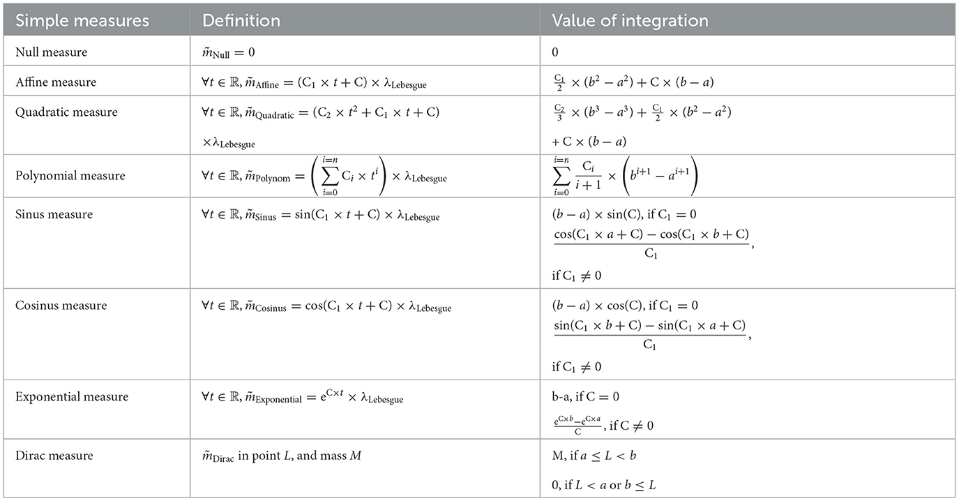
Table A1. Integration of some simple measures.

Simple fields

Table B1

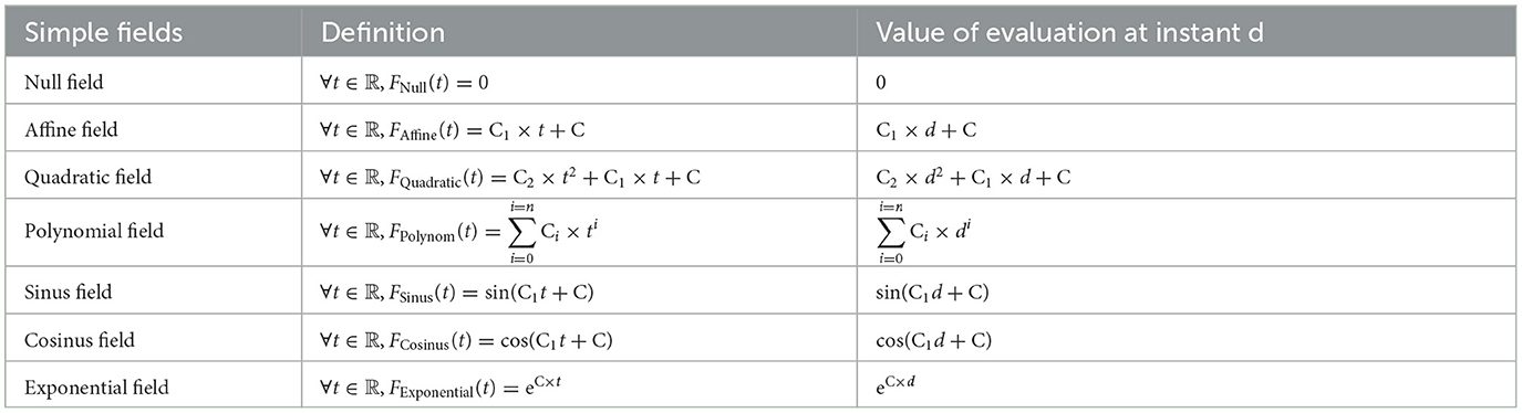
Table B1. Evaluation of some simple fields.