Automatic labeling of fish species using deep learning across different classification strategies

Convolutional neural networks (CNNs) have revolutionized image recognition. Their ability to identify complex patterns, combined with learning transfer techniques, has proven effective in multiple fields, such as image classification. In this article we propose to apply a two-step methodology for image classification tasks. First, apply transfer learning with the desired dataset, and subsequently, in a second stage, replace the classification layers by other alternative classification models. The whole methodology has been tested on a dataset collected at Conil de la Frontera fish market, in Southwest Spain, including 19 different fish species to be classified for fish auction market. The study was conducted in five steps: (i) collecting and preprocessing images included in the dataset, (ii) using transfer learning from 4 well-known CNNs (ResNet152V2, VGG16, EfficientNetV2L and Xception) for image classification to get initial models, (iii) apply fine-tuning to obtain final CNN models, (iv) substitute classification layer with 21 different classifiers obtaining multiple F1-scores for different training-test splits of the dataset for each model, and (v) apply post-hoc statistical analysis to compare their performances in terms of accuracy. Results indicate that combining the feature extraction capabilities of CNNs with other supervised classification algorithms, such as Support Vector Machines or Linear Discriminant Analysis is a simple and effective way to increase model performance.

1 Introduction

Convolutional neural networks (CNNs) have radically transformed the field of image processing and computer vision over the past decade. Leveraging their unique architecture, which mimics human visual processing, CNNs have consistently demonstrated their ability to extract intricate patterns and features from images, often outperforming human performance on specific tasks. This, together with data augmentation techniques—through rotation, zooming, panning, and other techniques—that allow the size and diversity of the training dataset to be expanded, is a well-established approach for similar tasks, widely recognized in the scientific community.

Several studies, such as those by Norouzzadeh et al. (2018), Allken et al. (2019), Barbedo (2019), Kaya et al. (2019), Montalbo and Hernandez (2019), and Palmer et al. (2022), highlight the effectiveness of CNNs in animal species classification. The adoption of pre-trained models such as ResNet-50, VGG16, and Xception underlines a fundamental trend in the deep learning community: transfer learning. Instead of training a model from scratch, researchers leverage pre-trained models on large datasets such as ImageNet to benefit from their already learned features. These models are then refined on specific datasets, often yielding superior results in a fraction of the original training time. We could highlight the following studies in this field ResNet-50 (He et al., 2016a), ResNet152V2 (He et al., 2016b), VGG16 (Simonyan and Zisserman, 2014), EfficientNetV2L (Tan and Le, 2021), Xception (Chollet, 2017), AlexNet (Krizhevsky et al., 2012), and GoogleNet (Szegedy et al., 2014).

The works cited employ a range of pre-trained models, each with its architecture and strengths. For instance, ResNet models, with their residual connections, are known to alleviate the vanishing gradient problem in deep networks (He et al., 2016a; Huang et al., 2017). On the other hand, EfficientNet architectures scale all dimensions of the model (width, depth, and resolution) based on a set compound coefficient, making them extremely efficient. These models, when paired with strategic data augmentation, can discern subtle differences among animal species, even those imperceptible to the human eye (Ibraheam et al., 2021).

Despite the prowess of CNNs, innovation in the field of machine learning continues unabated. The classification model presented in this paper represents this evolutionary process. Rather than relying solely on end-to-end training of CNNs, the model presented here employs a two-step process. First, feature extraction is performed using a CNN. These extracted features, rich in information content, are fed into a supervised learning model, which can be either a traditional machine learning algorithm or another neural network variant. This hybrid approach aims to harness the strength of CNNs in feature extraction and combine it with the robustness of other classification algorithms, potentially providing more accurate and interpretable results. Crucially, the selection of the definitive model will be based on a rigorous hypothesis testing process, ensuring that the chosen approach not only performs well in theory but also stands up to empirical scrutiny.

The supervised learning models used in this paper range from dimensionality reduction algorithms such as linear discriminant analysis (LDA) and quadratic discriminant analysis (QDA), through the generation of single and multiple decision trees, the latter known as Random Forest (RF), the use of Kernel methods such as support vector machines (SVM), the use of non-parametric classification methods such as the k-nearest neighbor (K-NN) algorithm and the use of probabilistic classification methods such as the Gaussian Naive Bayes (GNB) algorithm. All of them have been used independently for the classification of different biogeochemical species (Franco et al., 1990; Cutler et al., 2007; Munoz et al., 2013; Pundlik, 2016; Saberioon et al., 2018; Shang and Li, 2018; Deep and Dash, 2019; Knauer et al., 2019; Luan et al., 2020; Nuraini, 2022).

In essence, while CNNs have paved the way for unparalleled advancements in image classification, the ever-evolving landscape of machine learning ensures that newer, potentially more efficient methods will be needed.

Transfer learning is a common and effective approach in this field and has many advantages, such as a great reduction in training times and a better performance, specially for small datasets, where training from scratch may result in a severe overfitting. The usual approach consists on removing the final layers responsible for classification and replace them with new layers (usually fully-connected). The pre-trained model's weights are frozen, and only the weights of the new layers are trained on the specific dataset.

Previous models, which utilized the entire neural network, usually have a higher computational cost and possibly, a higher risk of overfitting when compared to some classic classification algorithms. The proposed technique allows for the exploration of different approaches and the identification of the classifier that best suits the characteristics of our data.

This work proposes a methodology for the design of a classification model using transfer learning and replacing the final layers by other alternative classifiers instead of using a set of fully-connected layers. In order to statistically assess the performance, a multiple comparison analysis has been applied to check whether there are differences in performance between the different classification models. This methodology has allowed to improve the generalization ability of the final model in a real-world scenario (fish market image recognition), getting a significant increase in performance.

2 Materials and methods

2.1 Dataset

The southern Spanish fish market has a rich history and a wide variety/range of seafood products. Most auction facilities, taking a leap toward modernity, have adopted digital platforms for their operations. These platforms primarily use photography to showcase their products to prospective buyers. However, by analysing these images, researchers can determine the size, species and weight, ensuring that fishing practices conform to sustainable standards. Many studies such as Dobeson (2016) and Jarek and Mazurek (2019) show that the integration of technological advances can significantly improve the traceability of sales and auction processes.

The dataset used for this study was gathered from sales conducted at the Conil de la Frontera (36°17'44.1”N 6°08'16.9”W) fish market, where each sold box is associated with an image. The images are captured within the sales box where only specimens of the same species of fish appear. Once the fishing vessel has unloaded its cargo and placed the catches in their sales boxes, they are transferred to a conveyor belt where they are weighed, and an image is captured for publication on the auction portal of the fish market. The photos have dimensions of 800 × 480 pixels with a resolution of 96 pixels per inch (ppi) at a fixed height of approximately 1 meter at the point where the box is weighed. Additionally, no additional lighting or flash is used beyond what is present in the room where these measurements are conducted.

These images are stored alongside auction sales data, including size, weight, and the Food and Agriculture Organization of the United Nations Code (FAO) which refers to the abbreviated nomenclature of the species, among other information, though private data of both buyers and sellers has been anonymized. The original raw dataset comprises 12,525 images representing 80 different species across 38 distinct days. However, there's a noticeable class imbalance issue, with some species having fewer than 30 sample images, while more common species such as those depicted in Figures 1A–D have 1.217, 2.167, 836 and 1.120 instances, respectively.

Figure 1

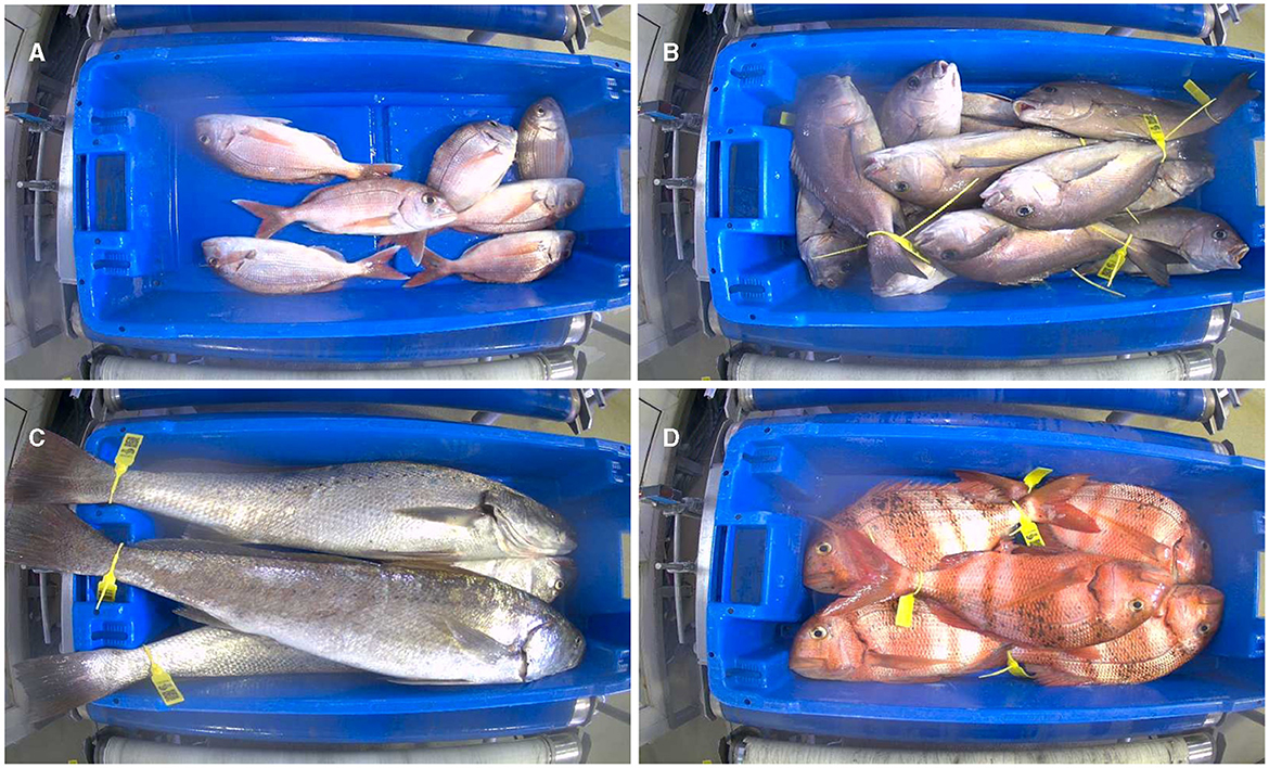
Figure 1. Main species of the fishing port of Conil de la Frontera. (A) Pagrus pagrus. (B) Plectorhinchus mediterraneus. (C) Argyrosomus regius. (D) Pagrus auriga.

To address class imbalance, the study focuses on the 19 species that have over 200 sales instances. The dataset is divided in a manner such that every species has 80% of their instances in training, 10% for validation and 10% for testing, henceforth keeping the balance in all the stages. Data augmentation techniques (Shorten and Khoshgoftaar, 2019) are applied to the training data, with the aim to increase instances for each species to a minimum of 500, greatly improving system performance. This approach enables the network to learn from image variations, including fish distribution, caliber differences, blood stains, camera water droplets, and snow in boxes, thus facilitating knowledge extrapolation. The original image set is retained, and new images are generated using transformations such as mirroring, rotation, blur, optical distortion, and hue-saturation adjustments. These are performed using the Albumentations framework (Buslaev et al., 2020), a Python library for fast and flexible image augmentations.

Therefore, the resulting dataset consists of 10,632 instances, representing 19 target species, with an average of 640 images per class. Furthermore, 20% of the dataset is reserved for test and validation purposes. Therefore, it is divided into training (80%–8,505 original instances, 12,095 with data augmentation), validation (10%–1,064 instances), and testing (10%-1,063 instances).

As established in the introduction, this study aims to conduct a comparative analysis among various classification models based on convolutional neural networks (CNNs) and distinct supervised learning models that do not utilize neural networks for classification.

2.2 CNN models and supervised learning

A CNN is a deep learning model designed for the processing of grid-structured data, such as images or matrix data. In contrast to conventional neural networks, CNNs employ a specialized architecture that leverages the spatial correlations in data by applying convolutional filters across successive layers (Goodfellow et al., 2016). These filters autonomously acquire local features, such as edges, textures, and shapes, which accumulate to construct increasingly abstract and meaningful representations as one delves deeper into the network.

One of the main advantages of CNNs is their inherent capacity to autonomously extract features from input data without necessitating prior preprocessing. Instead of requiring the manual design and selection of pertinent features for a specific task, CNNs dynamically and hierarchically acquire the most discriminative features during the training process. This attribute renders them exceptionally potent for various computer vision tasks, including but not limited to image classification, object detection, segmentation, and face recognition.

Pre-trained networks refer to CNN models that have undergone training on extensive datasets, such as ImageNet, and have garnered widespread popularity within the deep learning community (Hussain et al., 2019). The current study will employ these pre-trained models, including ResNet152V2 (He et al., 2016b), VGG16 (Simonyan and Zisserman, 2014), EfficientNetV2L (Tan and Le, 2021), and Xception (Chollet, 2017), as a foundation. These models have acquired the ability to discern a diverse array of visual features, rendering them a robust basis for various computer vision tasks. By harnessing the wealth of knowledge embedded in these models, substantial time and resources can be conserved, as there is no need to initiate training from scratch, leading to expedited access to high-quality results.

Let the VGG16 CNN architecture shown in Figure 2 work as an example. It can't be used without applying transfer learning (Goodfellow et al., 2016), a technique used to extrapolate pre-trained CNN models to new classification problems. CNNs can be divided in two main parts: the convolution layers where the feature extraction is performed, and the fully connected layers (Multi Layer Perceptron MLP) where the classification is performed based on the features extracted. Since the original number of classes is different of ours, the last part of the CNN architecture is replaced with a new Fully Connected Neural Network (FCNN) which matches our number of fish species, 19.

Figure 2

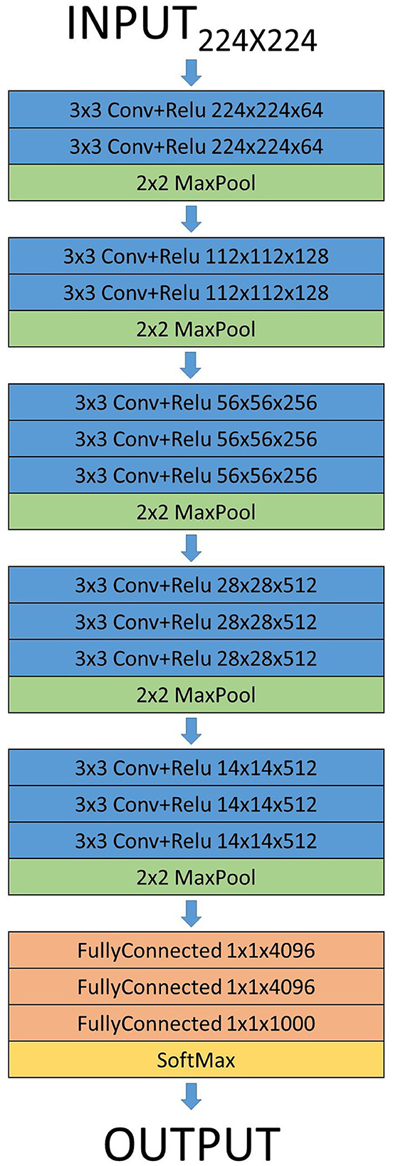
Figure 2. VGG16 CNN architecture. An input image of size 224 × 224 is supplied, followed by a sequence of convolutional and pooling layers, culminating in a single hidden layer comprising 4,096 neurons that feed into the output classification layer for the desired number of classes. When applying transfer learning, only the input layer and the final fully-connected layer are modified.

The initial feature extraction layers remain unchanged, as they retain the knowledge acquired from the ImageNet dataset. However, the classification layers are substituted with a GlobalAveragePooling2D layer followed by a Dense-Softmax output layer which will serve as the classification layer.

To perform the comparison, the same number of features has been employed for all algorithms. These features are extracted by the CNN models in their convolutional stage. Given this, VGG16 results in 14 × 14 × 512 = 100,352 (as seen in Figure 2) neurons after the final pooling and flattening of neurons across all convolutional layers. Therefore, it will be the number of features extracted by VGG16 for the comparison among all supervised learning models. Ultimately, the goal is to utilize the feature extractor of CNN models in their convolutional stage, which was employed in the fully-connected layers of the original model for the classification, as a feature extractor that will feed the features to the supervised learning models. Thus, within the same CNN model, comparisons are made with the same number of extracted features, and among different CNN models, the number of these features will vary.

The workflow for training and validating the models is outlined in Algorithm 1. The system begins by initially training and evaluating the proposed CNN-based model. Subsequently, the final classification layers are removed, and the model's output is set to the features extracted from the convolutional layers. This modified model is then used as a feature extractor for the proposed supervised learning classifier models.

Algorithm 1

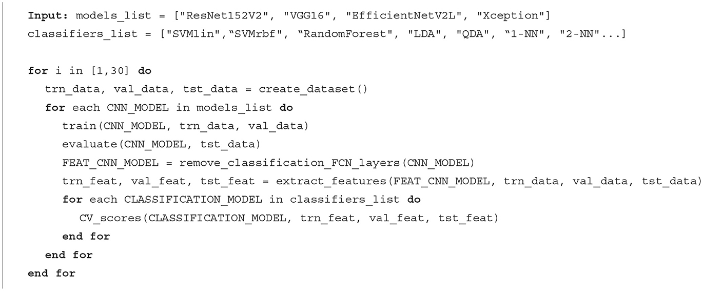
Algorithm 1. Workflow for training and validation.

During the supervised learning process, all images are preprocessed using the feature extractor obtained from the original CNN, which will serve as input for the proposed models. The results of each combination of the CNN model and the supervised learning model are evaluated through the mean of five executions of 10-fold Cross-Validation. The algorithms employed are those mentioned in the Introduction, namely: Linear Support Vector Machine (SVM), Radial kernel SVM, Polynomial SVM, Random Forest, Linear Discriminant Analysis (LDA), Quadratic Discriminant Analysis, Gaussian Bayes, Decision Tree, and K-NN with K values ranging from 1 to 29 in steps of 2.

Therefore, we have a total of 23 algorithms and 4 pre-trained CNN models, resulting in 23·4+4 = 96 distinct models. The remaining 4 models correspond to the original CNN+MLP (CNN with a classification layer based on a MLP) models that were trained separately.

2.3 Model training and evaluation

In this work, the training and evaluation of all models was developed in Python 3.10 using the scikit-learn package v1.2.2. From this package, four modules were used for modeling (tree, neural_networks, mixture, and ensemble), while the metrics module was used for performance calculations. Since the Transfer Learning technique has been used, the training stage is performed in two phases in order to improve the performance of the results. First, the convolutional layers of the model are frozen so that the training will affect just the Fully Connected (FC) layers. We use “categorical crossentropy” as the loss function and the Adam optimizer with its default hyperparameters of learning rate and decay (Goodfellow et al., 2016). The model is trained in 35 epochs and with a batch size of 64. The batch size has been selected to ensure optimal placement of the model within the GPU's shared memory. Using a larger batch size would risk memory overflow, while a smaller batch size tends to result in overfitting. The GPU is an NVIDIA GeForce RTX 3090Ti with 24GiB of memory, of which 22.4GiB is used for model storage.

Once the model has been fully trained with these parameters, a fine-tuning training phase is performed in order to adapt the whole network to this specific problem and increase its performance. In this stage, all the layers are unfrozen, so that the training changes all the weights of the model. However, a low learning rate, specifically 1e-5, is set to ensure only minor adjustments are made to the model's weights, avoiding drastic changes. Furthermore, as we are updating all layers, the size of the model in the GPU increases, necessitating a reduction in the batch size to 16. All these parameters are shown at Table 1. The selection of values is motivated by hyperparameter tuning through grid search, aiming to enhance the f-score and reduce the training time for all proposed CNN models.

Table 1

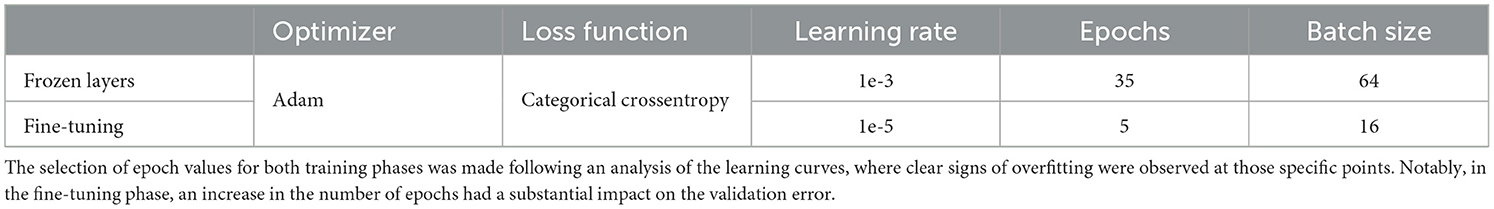
Table 1. Training hyperparameters summary: the batch size was chosen according to the memory constraints of the GPU.

To assess the performance of our model, we will focus on the concept of model evaluation, with a particular emphasis on its relevance to CNN models. We will delve into the common metric used to gauge the effectiveness of CNNs in various computer vision tasks, providing crucial insights into their object classification capabilities. By comprehending and interpreting these evaluation metric, we can make informed decisions concerning model selection, optimization, and deployment. The performance of our models will be quantified using the mean F₁-Score of all the species, which is defined by Equations 1–3:

$\begin{array}{ll}Precision=\frac{TP}{TP+FP}& (1)\end{array}$

$\begin{array}{ll}Recall=\frac{TP}{TP+FN}& (2)\end{array}$

$\begin{array}{ll}{F}_{1}Score=2·\frac{precision·recall}{precision+recall}& (3)\end{array}$

Where TP stands for True Positives, FP for False Positives and FN as False Negatives.

For a correct evaluation of the proposed models, we carefully assembled a total of 30 distinct datasets, dividing each one into training, validation, and test sets. First, each model was trained using the training and validation sets and the F1 metric was then calculated using test data for each dataset. Finally, the average F1-score was obtained. This method enables us to cover a diverse array of scenarios, representing various sets of instances that can be fed into the network, and statistically demonstrate the performance of the models. Henceforth, the metrics presented for each experiment are the outcomes of 30 iterations of each proposed model.

3 Results and discussion

This section presents the results from 30 executions of the 96 proposed models. Among these, four are associated with the original CNN+MLP pretrained CNN models, while the remaining 92 pertain to the CNN+supervised learning proposed algorithms. The final objective of this work is to perform a well-founded comparison between the proposed models. To achieve this, we employ the comparative model analysis discussed in Pizarro et al. (2002). This paper introduces a novel approach to model selection that is based on hypothesis testing.

When comparing the models, the first thing that comes to mind is to determine whether there are statistically significant differences between the means. In this case, the usual approach is apply Analysis of Variance (ANOVA). However, ANOVA has a number of assumptions that should hold for valid inferences: normality, homoscedasticity(uniform variance across all groups) and independence of cases among others.

The Shapiro-Wilk test is a well-known test to evaluate whether the dataset is normally distributed within each model. If the p-value obtained exceeds the significance level, the null hypothesis (the population is normally distributed) cannot be rejected. This test is applied to each group, so the test generates a p-value for each of the models, allowing us to determine which models individually adhere to a normal distribution. With a significance level of 0.01, it was obtained that all p-values were greater than 0.01, and the null hypothesis for each group that the data are normally distributed could not be rejected.

The second tested assumption was the homogeneity of variances. In this case, the Levene test was conducted with the null hypothesis that the variances of all groups are equal. The Levene test applied to all groups gave a p-value of 3.4154e-70, leading to the rejection of the null hypothesis, indicating the presence of different variances among the groups.

Post hoc tests, such as Bonferroni (1936), Tukey (1949), Duncan (1955), Dunnett (1955), etc. Galindo et al. (2000) allow testing for differences between multiple group means while also controlling for the family-wise error rate, that is, the probability of at least one false conclusion in a series of hypothesis tests. However, most of these tests rely on the equal variance assumption. When the homoscedasticity assumption is not met, which was our case, alternative tests might be used. In such situation, the Games-Howell, Tamhane's T2, Dunnett's T3, and Dunnett's C tests can be applied (Shingala and Rajyaguru, 2015). The Games-Howell test is similar to Tukey's test, but it does not assume equal variances and sample sizes (provided that there are more than five samples in each group) (Games et al., 1979). In our case, this last prerequisite is also easily met, as there are 30 runs for each model. The Games-Howell used routine performs a pairwise comparison among groups which returns a p-value bounded between 0.001 and 0.9. This is due to the fact that the calculation of the p-value uses scalar minimization and results are bound to be between 0.001 and 0.9, as described in the documentation of statsmodel package (Seabold and Perktold, 2010). Therefore, a p-value = 0.001 in the results should be interpreted as p-value ≤ 0.001, and a p-value = 0.9 should be interpreted as p-value ≥ 0.9.

Consequently, a pairwise model comparison using Games-Howell routine was conducted among the CNN-MLP models (see Table 2) using four different pre-trained models (EfficientNetV2L, ResNet152V2, VGG16, and Xception). From the results, there is no evidence that EfficientNetV2L and VGG16 are significantly distinguishable from each other (p-value ≥ 0.9), as it happens with ResNet152V2 and Xception (p-value ≥ 0.9). However, these pairs are significantly distinguishable from each other(p-value ≤ 0.01), resulting in two distinct pairs of models, with one pair apparently outperforming the other (see Figure 3). The boxplot displays the sample distribution for each model. It is also notable that the models' variances are not equal; EfficientNetV2L and VGG16 exhibit notably different standard deviations, being VGG16 results more dispersed than those obtained by EfficientNetV2L.

Table 2

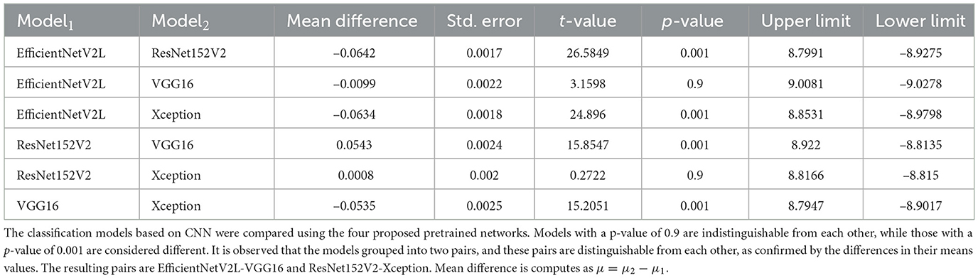
Table 2. Multiple models are subjected to pairwise comparisons using the Games-Howell test.

Figure 3

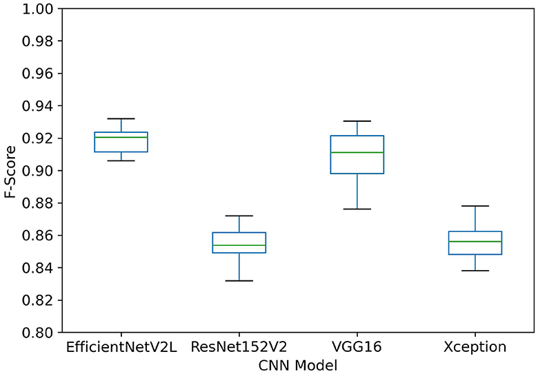
Figure 3. Sample distribution for F-Score results using CNN-MLP models. It is observed that EfficientNetV2L and VGG16 get better results, while ResNet152V2 and Xception results are not so competitive, in good agreement with the statistical analysis results. It is also evident that the variances of the distributions of F-score for each model are not equal (i.e., VGG16 clearly shows a more dispersed distribution than EfficientNetV2L).

Finally, the CNN-MLP models were compared with their sub-models using supervised learning algorithms for classification to determine which ones serve as the best classifiers. We validated models that, while demonstrating a better average than their MLP classifier counterparts, were significantly distinct from them. Therefore, it was observed that four sub-models had significantly better performance than the MLP version (see Table 3 and Figure 4). Models employing SVM or LDA algorithms have shown improved performance compared to their MLP versions, with an average F-Score enhancement of 0.03. Furthermore, these four models are deemed significantly distinguishable from the MLP model while also being statistically indistinguishable from each other.

Table 3

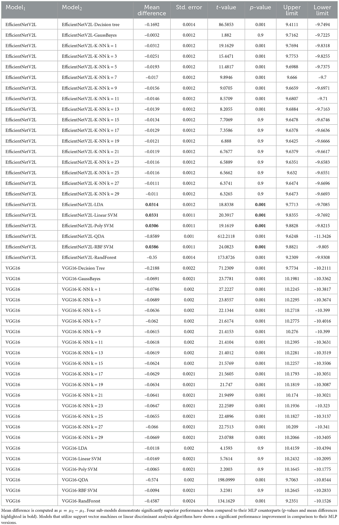
Table 3. Games-Howell model comparison for the top CNN+MLP models, in comparison with their sub-models utilizing supervised learning algorithms for classification results.

Figure 4

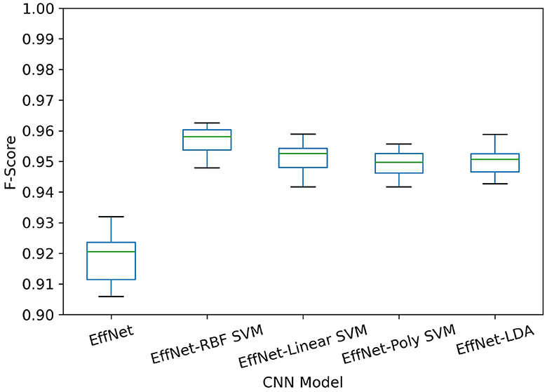
Figure 4. Sample distribution for F-score results using EfficientNetV2L model (shown as “EffNet”), CNN+MLP and four sub-models that exhibit significantly better performance than the MLP version (see Table 3) models are shown. Models employing SVM or LDA classification algorithms have shown improved performance compared to their MLP versions. This statistically proven improvement is clearly evident in the figure, where models utilizing the proposed supervised learning algorithms exhibit a higher mean and a more concentrated distribution of F-Score.

The F-Score performance of various models was assessed through 30 independent executions (Tables 4, 5). Notably, the EfficientNetV2L and VGG16 models are presented as they are deemed statistically superior in F-Score performance compared to the other proposed models (refer to Table 2). Models with statistically indistinguishable performance are emphasized. It can be seen that these highlighted models distinctly outperform the others; the minimum value achieved by these models exceeds the maximum of the remaining models by 0.01, as demonstrated by the maximum achieved by EfficientNetV2L. Consequently, the results obtained from the Games-Howell comparison (refer to Table 3) are considered representative proposed models' performance.

Table 4

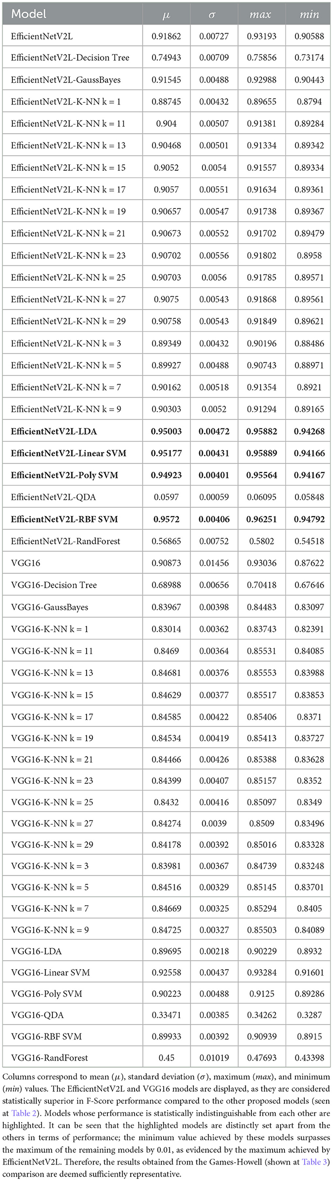
Table 4. F-Score performance obtained by different models in 30 independent executions.

Table 5

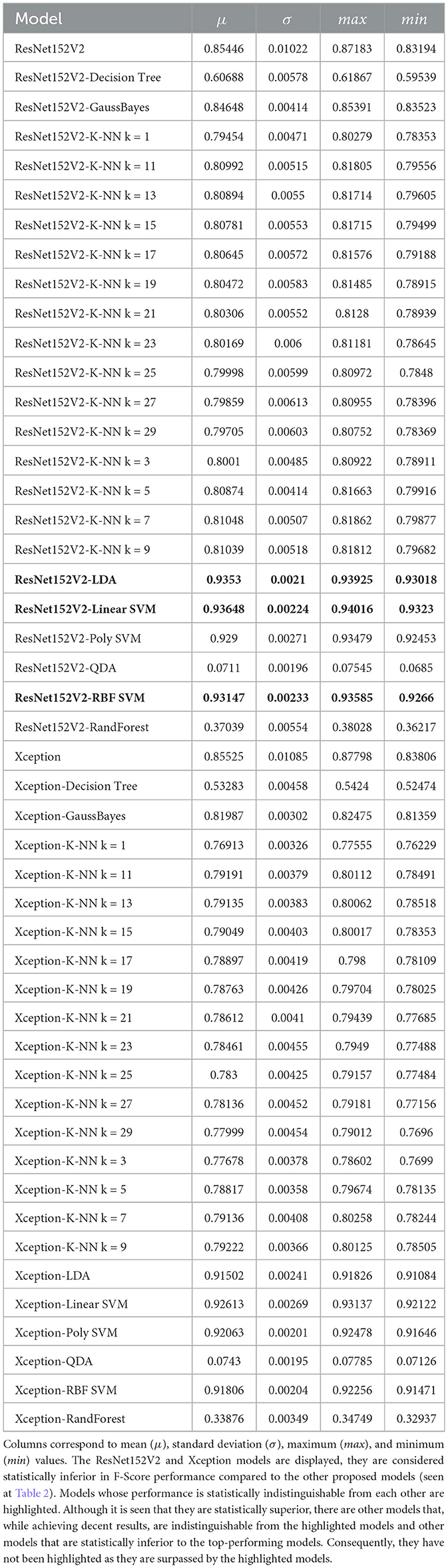
Table 5. F-Score performance obtained by different models in 30 independent executions.

4 Conclusions

In this research paper, we have tackled the challenging task of automating the labeling of fish species through the application of deep learning techniques. Specifically, we examined the efficacy of four different pre-trained neural networks, including ResNet, VGG16, EfficientNetV2L, and Xception, using transfer learning. After transfer learning, we harnessed the knowledge these networks had gained from large-scale datasets and fine-tune them to our specific fish image dataset.

The initial phase of our investigation involved transfer learning, where all the pre-trained layers were kept frozen, allowing only the last layer to be customized to our dataset. Subsequently, we employed fine-tuning, which permitted us to update the pre-trained layers. This two-step approach aimed to leverage the powerful representations learned by these networks while adapting them to the nuances of our fish image dataset.

To further enhance the performance of our system, we decided to replace the final layers of the pre-trained networks with 23 distinct classification models, including Support Vector Machines (SVM), Linear Discriminant Analysis (LDA), Random Forests, and k-Nearest Neighbors (K-NN), among others. This diverse set of classifiers allowed us to explore which model might be most suitable for the classification task using the features extracted from the pre-trained CNN.

To determine the best-performing model among the extensive pool of candidates, we conducted a rigorous comparative analysis. It's worth noting that we encountered a deviation from the homoscedasticity assumption in our data. To address this issue, we applied the Games-Howell method, which is an improved and robust alternative to the Tukey-Kramer method. The Games-Howell method was specifically selected because of its suitability for scenarios where the homoscedasticity assumption is violated.

Our comparative analysis, rooted in the Games-Howell test, has demonstrated that not all pre-trained networks are created equal when it comes to fish species recognition. Specifically, EfficientNet and VGG16 emerged as the top performers, significantly outshining ResNet and Xception in our dataset. This highlights the importance of carefully selecting a pre-trained network that aligns with the specific nuances of the task at hand, and it underscores that not all deep learning architectures are universally applicable.

Moreover, our exploration of the final stage of the CNN architecture revealed a promising strategy for performance enhancement. The integration of classifiers like SVM and LDA as the concluding layer of the CNN framework led to a substantial improvement in the F-score, namely, from 0.92 to 0.95. This result suggests that the incorporation of sophisticated classifiers can serve as a powerful tool to boost the accuracy and reliability of CNNs in image classification tasks. This strategy should certainly be considered and explored in similar cases, opening up opportunities for enhancing the capabilities of deep learning models in a variety of applications.

Lastly, the comparison between the CNN-MLP models and their sub-models employing supervised learning algorithms unveiled a set of four models that exhibited significantly superior performance to their MLP counterparts. The integration of support vector machines and linear discriminant analysis algorithms led to an average F-score enhancement of 0.03, showcasing the potential of these classifiers in image classification tasks.

We may conclude that our study provides valuable insights into the intricate world of deep learning and image classification, emphasizing the importance of model selection, the strategic integration of classifiers, and the careful consideration of statistical testing techniques. These findings not only contribute to the field of automatic fish species labeling but also offer a roadmap for researchers in diverse domains seeking to leverage deep learning and statistical analysis to enhance their own classification tasks. This work paves the way for more robust and efficient approaches to image classification and serves as a foundation for further exploration in the realm of computer vision and machine learning.

Data availability statement

The original contributions presented in the study are included in the article/supplementary material, further inquiries can be directed to the corresponding author.

Ethics statement

Ethical approval was not required for the study involving animals in accordance with the local legislation and institutional requirements because the research was made on photographs obtained at fish market.

Author contributions

JJ: Conceptualization, Data curation, Formal analysis, Investigation, Methodology, Project administration, Resources, Software, Validation, Visualization, Writing—original draft, Writing—review & editing. GB-G: Conceptualization, Data curation, Formal analysis, Investigation, Methodology, Resources, Software, Validation, Visualization, Writing—original draft, Writing—review & editing. JC-G: Investigation, Validation, Writing—review & editing. RC-C: Funding acquisition, Investigation, Resources, Validation, Writing—review & editing. PG: Conceptualization, Data curation, Formal analysis, Funding acquisition, Investigation, Methodology, Project administration, Resources, Software, Supervision, Validation, Visualization, Writing—original draft, Writing—review & editing.

Funding

The author(s) declare financial support was received for the research, authorship, and/or publication of this article. The work was supported by “Ministerio de Agricultura, Pesca y Alimentación–Fondos NextGenerationEU” (DIGIPESCA Project) and “Junta de Andalucía–Grupos PAI” (TIC-145 and RNM-243 Research Groups).

Acknowledgments

The authors would like to thank the Lonja de Conil (fish market) for providing the data used in this research.

Conflict of interest

The authors declare that the research was conducted in the absence of any commercial or financial relationships that could be construed as a potential conflict of interest.

Publisher's note

All claims expressed in this article are solely those of the authors and do not necessarily represent those of their affiliated organizations, or those of the publisher, the editors and the reviewers. Any product that may be evaluated in this article, or claim that may be made by its manufacturer, is not guaranteed or endorsed by the publisher.

References

Allken, V., Handegard, N. O., Rosen, S., Schreyeck, T., Mahiout, T., and Malde, K. (2019). Fish species identification using a convolutional neural network trained on synthetic data. ICES J. Mar. Sci. 76, 342–349. doi: 10.1093/icesjms/fsy147

Crossref Full Text | Google Scholar

Barbedo, J. G. A. (2019). Plant disease identification from individual lesions and spots using deep learning. Biosyst. Eng. 180, 96–107. doi: 10.1016/j.biosystemseng.2019.02.002

Crossref Full Text | Google Scholar

Bonferroni, C. E. (1936). Teoria statistica delle classi e calcolo delle probabilita. Pubbl. R. Ist. Super. di Sci. Econom. Commer. Firenze. 8, 3–62.

Google Scholar

Buslaev, A., Iglovikov, V. I., Khvedchenya, E., Parinov, A., Druzhinin, M., and Kalinin, A. A. (2020). Albumentations: fast and flexible image augmentations. Information 11:125. doi: 10.3390/info11020125

Crossref Full Text | Google Scholar

Chollet, F. (2017). “Xception: deep learning with depthwise separable convolutions,” in Proceedings of the IEEE Conference on Computer Vision and Pattern Recognition 1251–1258. doi: 10.1109/CVPR.2017.195

Crossref Full Text | Google Scholar

Cutler, D. R., Edwards Jr, T. C., Beard, K. H., Cutler, A., Hess, K. T., Gibson, J., et al. (2007). Random forests for classification in ecology. Ecology 88, 2783–2792. doi: 10.1890/07-0539.1

PubMed Abstract | Crossref Full Text | Google Scholar

Deep, B. V., and Dash, R. (2019). “Underwater fish species recognition using deep learning techniques,” in 2019 6th International Conference on Signal Processing and Integrated Networks (SPIN) (IEEE), 665–669. doi: 10.1109/SPIN.2019.8711657

Crossref Full Text | Google Scholar

Dobeson, A. (2016). Scopic valuations: how digital tracking technologies shape economic value. Econ. Soc. 45, 454–478. doi: 10.1080/03085147.2016.1224143

Crossref Full Text | Google Scholar

Duncan, D. B. (1955). Multiple range and multiple f tests. Biometrics 11, 1–42. doi: 10.2307/3001478

Crossref Full Text | Google Scholar

Dunnett, C. W. (1955). A multiple comparison procedure for comparing several treatments with a control. J. Am. Stat. Assoc. 50, 1096–1121. doi: 10.1080/01621459.1955.10501294

Crossref Full Text | Google Scholar

Franco, M., Seeber, R., Sferlazzo, G., and Leardi, R. (1990). Classification and prediction ability of pattern recognition methods applied to sea-water fish. Analyt. Chim. Acta 233, 143–147. doi: 10.1016/S0003-2670(00)83471-6

Crossref Full Text | Google Scholar

Galindo, P. L., Pizarro-Junquera, J., and Guerrero, E. (2000). “Multiple comparison procedures for determining the optimal complexity of a model,” in Advances in Pattern Recognition: Joint IAPR International Workshops SSPR 2000 and SPR 2000 Alicante, Spain, August 30-September 1, 2000 Proceedings (Springer), 796–805. doi: 10.1007/3-540-44522-6_82

Crossref Full Text | Google Scholar

Games, P. A., Keselman, H. J., and Clinch, J. J. (1979). Tests for homogeneity of variance in factorial designs. Psychol. Bull. 86:978. doi: 10.1037//0033-2909.86.5.978

Crossref Full Text | Google Scholar

Goodfellow, I., Bengio, Y., and Courville, A. (2016). Deep Learning. London: MIT press.

Google Scholar

He, K., Zhang, X., Ren, S., and Sun, J. (2016a). “Deep residual learning for image recognition,” in Proceedings of the IEEE Conference on Computer Vision and Pattern Recognition 770–778. doi: 10.1109/CVPR.2016.90

Crossref Full Text | Google Scholar

He, K., Zhang, X., Ren, S., and Sun, J. (2016b). “Identity mappings in deep residual networks,” in Computer Vision-ECCV 2016: 14th European Conference, Amsterdam, The Netherlands, October 11–14, 2016, Proceedings, Part IV (Springer), 630–645. doi: 10.1007/978-3-319-46493-0_38

Crossref Full Text | Google Scholar

Huang, G., Liu, Z., Van Der Maaten, L., and Weinberger, K. Q. (2017). “Densely connected convolutional networks,” in Proceedings of the IEEE Conference on Computer Vision and Pattern Recognition 4700–4708. doi: 10.1109/CVPR.2017.243

Crossref Full Text | Google Scholar

Hussain, M., Bird, J. J., and Faria, D. R. (2019). “A study on cnn transfer learning for image classification,” in Advances in Computational Intelligence Systems: Contributions Presented at the 18th UK Workshop on Computational Intelligence, September 5–7, 2018, Nottingham, UK (Springer), 191–202. doi: 10.1007/978-3-319-97982-3_16

Crossref Full Text | Google Scholar

Ibraheam, M., Li, K. F., Gebali, F., and Sielecki, L. E. (2021). A performance comparison and enhancement of animal species detection in images with various R-CNN models. AI 2, 552–577. doi: 10.3390/ai2040034

Crossref Full Text | Google Scholar

Jarek, K., and Mazurek, G. (2019). Marketing and artificial intelligence. Central Eur. Bus. Rev. 8, 46–55. doi: 10.18267/j.cebr.213

Crossref Full Text | Google Scholar

Kaya, A., Keceli, A. S., Catal, C., Yalic, H. Y., Temucin, H., and Tekinerdogan, B. (2019). Analysis of transfer learning for deep neural network based plant classification models. Comput. Electr. Agric. 158, 20–29. doi: 10.1016/j.compag.2019.01.041

Crossref Full Text | Google Scholar

Knauer, U., von Rekowski, C. S., Stecklina, M., Krokotsch, T., Pham Minh, T., Hauffe, V., et al. (2019). Tree species classification based on hybrid ensembles of a convolutional neural network (CNN) and random forest classifiers. Rem. Sens. 11, 2788. doi: 10.3390/rs11232788

Crossref Full Text | Google Scholar

Krizhevsky, A., Sutskever, I., and Hinton, G. E. (2012). “Imagenet classification with deep convolutional neural networks,” in Advances in Neural Information Processing Systems 25.

Google Scholar

Luan, J., Zhang, C., Xu, B., Xue, Y., and Ren, Y. (2020). The predictive performances of random forest models with limited sample size and different species traits. Fisher. Res. 227:105534. doi: 10.1016/j.fishres.2020.105534

Crossref Full Text | Google Scholar

Montalbo, F. J., and Hernandez, A. (2019). “Classification of fish species with augmented data using deep convolutional neural network,” in 2019 IEEE 9th International Conference on System Engineering and Technology (ICSET) (IEEE), 396–401. doi: 10.1109/ICSEngT.2019.8906433

Crossref Full Text | Google Scholar

Munoz, F., Pennino, M. G., Conesa, D., Lopez-Quilez, A., and Bellido, J. M. (2013). Estimation and prediction of the spatial occurrence of fish species using bayesian latent gaussian models. Stochastic Environ. Res. Risk Assess. 27, 1171–1180. doi: 10.1007/s00477-012-0652-3

Crossref Full Text | Google Scholar

Norouzzadeh, M. S., Nguyen, A., Kosmala, M., Swanson, A., Palmer, M. S., Packer, C., et al. (2018). Automatically identifying, counting, and describing wild animals in camera-trap images with deep learning. Proc. Natl. Acad. Sci. 115, E5716–E5725. doi: 10.1073/pnas.1719367115

PubMed Abstract | Crossref Full Text | Google Scholar

Nuraini, R. (2022). Identification of freshwater fish types using linear discriminant analysis (lda) algorithm. IJICS 6, 147–154. doi: 10.30865/ijics.v6i3.5565

Crossref Full Text | Google Scholar

Palmer, M., Álvarez Ellacuría, A., Moltó, V., and Catalán, I. A. (2022). Automatic, operational, high-resolution monitoring of fish length and catch numbers from landings using deep learning. Fisher. Res. 246:106166. doi: 10.1016/j.fishres.2021.106166

Crossref Full Text | Google Scholar

Pizarro, J., Guerrero, E., and Galindo, P. L. (2002). Multiple comparison procedures applied to model selection. Neurocomputing 48, 155–173. doi: 10.1016/S0925-2312(01)00653-1

Crossref Full Text | Google Scholar

Pundlik, R. (2016). “Comparison of sensitivity for consumer loan data using gaussian naïve bayes (gnb) and logistic regression (lr),” in 2016 7th International Conference on Intelligent Systems, Modelling and Simulation (ISMS) (IEEE), 120–124. doi: 10.1109/ISMS.2016.57

Crossref Full Text | Google Scholar

Saberioon, M., Císař, P., Labbé, L., Souček, P., Pelissier, P., and Kerneis, T. (2018). Comparative performance analysis of support vector machine, random forest, logistic regression and k-nearest neighbours in rainbow trout (oncorhynchus mykiss) classification using image-based features. Sensors 18:1027. doi: 10.3390/s18041027

PubMed Abstract | Crossref Full Text | Google Scholar

Seabold, S., and Perktold, J. (2010). “Statsmodels: econometric and statistical modeling with python,” in Proceedings of the 9th Python in Science Conference (Austin, TX), 10–25080. doi: 10.25080/Majora-92bf1922-011

Crossref Full Text | Google Scholar

Shang, Y., and Li, J. (2018). “Study on echo features and classification methods of fish species,” in 2018 10th International Conference on Wireless Communications and Signal Processing (WCSP) (IEEE), 1–6. doi: 10.1109/WCSP.2018.8555591

Crossref Full Text | Google Scholar

Shingala, M. C., and Rajyaguru, A. (2015). Comparison of post hoc tests for unequal variance. Int. J. New Technol. Sci. Eng. 2, 22–33. Available online at: https://www.ijntse.com/upload/1447070311130.pdf

Google Scholar

Shorten, C., and Khoshgoftaar, T. M. (2019). A survey on image data augmentation for deep learning. J. Big Data 6, 1–48. doi: 10.1186/s40537-019-0197-0

Crossref Full Text | Google Scholar

Simonyan, K., and Zisserman, A. (2014). Very deep convolutional networks for large-scale image recognition. arXiv preprint arXiv:1409.1556.

Google Scholar

Szegedy, C., Liu, W., Jia, Y., Sermanet, P., Reed, S., Anguelov, D., et al. (2014). “Going deeper with convolutions,” in Proceedings of the IEEE Conference on Computer Vision and Pattern Recognition 1–9. doi: 10.1109/CVPR.2015.7298594

Crossref Full Text | Google Scholar

Tan, M., and Le, Q. (2021). “Efficientnetv2: smaller models and faster training,” in International Conference on Machine Learning (PMLR), 10096–10106.

Google Scholar

Tukey, J. W. (1949). Comparing individual means in the analysis of variance. Biometrics 5, 99–114. doi: 10.2307/3001913

Crossref Full Text | Google Scholar