Orthogonality and graph divergence losses promote disentanglement in generative models

Over the last decade, deep generative models have evolved to generate realistic and sharp images. The success of these models is often attributed to an extremely large number of trainable parameters and an abundance of training data, with limited or no understanding of the underlying data manifold. In this article, we explore the possibility of learning a deep generative model that is structured to better capture the underlying manifold's geometry, to effectively improve image generation while providing implicit controlled generation by design. Our approach structures the latent space into multiple disjoint representations capturing different attribute manifolds. The global representations are guided by a disentangling loss for effective attribute representation learning and a differential manifold divergence loss to learn an effective implicit generative model. Experimental results on a 3D shapes dataset demonstrate the model's ability to disentangle attributes without direct supervision and its controllable generative capabilities. These findings underscore the potential of structuring deep generative models to enhance image generation and attribute control without direct supervision with ground truth attributes signaling progress toward more sophisticated deep generative models.

1 Introduction

Data-driven deep learning techniques have resulted in numerous advances, but several findings have demonstrated the brittleness of such models in different end tasks (Nguyen et al., 2015; Pontin, 2018). Many reasons have been hypothesized for such empirical behavior, chief among which is the realization that there is a need to leverage known physical laws such as the physics of image formation, the interaction of light with surfaces, and disentangling the effects of intrinsic object-related shape from photometric variation into deep learning frameworks (Bronstein et al., 2017). Several studies show that even simple unaccounted for shifts in data can lead to large losses in performance. Furthermore, from information theoretic perspectives (Achille and Soatto, 2018), the concepts of invariance and task performance are considered at odds with each other (e.g., discrimination). Information theoretic metrics for invariance seek to reduce the dimension of representations (Achille and Soatto, 2018), whereas metrics for a specific end-task such as classification seem to benefit from larger representation dimension. Thus, it seems that one cannot achieve true invariance while maintaining high end-task performance nor can one achieve high end-task performance while guaranteeing invariance. Information theoretic analysis suggests the need for a middle ground, where a geometric treatment of feature spaces and loss functions can potentially allow deep representations to find practical tradeoffs between task performance and invariance. When applied to generative models, invariance often refers to achieving a clean disentanglement of control variables–that correspond specifically to physical factors, such as pose, lighting, and shape–where modifying the control variable can be done in isolation, without affecting other variables.

In vision literature, much prior knowledge exists about how light interacts with surface geometry and reflectance properties, the workings of projective geometry, and how temporal dynamics can be used to explain observed dynamic scenes. These physical laws and properties constrain the set of feasible or valid observations from image sensors. Images are often constrained to lie in low-dimensional subsets (of large Euclidean spaces), more formally referred to as image manifolds. While numerous efforts have sought to characterize these image manifolds, both empirically and theoretically, throughout the last two decades (Turaga and Srivastava, 2015; Shao et al., 2018), how they are integrated into controllable and disentangled generative architectures is still an open question. In prior study (Shukla et al., 2019), we have shown that several of these constraint sets can be relaxed to subspace-type or sphere-type constraints. Different such constraints can be accommodated by constraining the features from the latent space to have orthogonality properties, as a proxy for physical factor disentanglement.

In the context of generative models, while there exist many different classes of architectures, a common theme is to learn the underlying distribution of the dataset. Once trained, it can be used to sample novel data points from the underlying distribution. There are diverse types of generative models, including but not limited to generative adversarial networks (GANs; Goodfellow et al., 2014) and variational autoencoders (VAEs; Kingma and Welling, 2013), each with pros and cons. These generative models generally have a low-dimensional latent space modeled using a Gaussian or uniform distribution, and they map these low-dimensional points to complex high-dimensional data points, matching the distribution of the training dataset. Generative models are versatile and used in various applications such as text-to-image models (Zhang et al., 2023), image-to-image translation (Zhu et al., 2017), domain adaptation (Hoffman et al., 2018), image editing (Zhu et al., 2020), and inverse problems (Asim et al., 2020). Furthermore, these generative models can offer explainable and controllable representation, leading to disentangled representations, a key area of interest. How do we encode the geometric nature of the output space in the loss function of generative model is still an open question. In this article, we make some concerted advances toward that via manifold-divergence loss functions and latent-space orthogonality properties.

One major challenge in existing approaches is the trade off between their ability to disentangle different attributes and their ability to generate novel samples. Most existing studies are based on VAEs and GANs that encourage factorization of the latent space. Methods based on VAE add a regularizer to the loss function to encourage disentanglement in the encoder distribution. Owing to their ability to capture explainable and controllable representation, they have been used in applications in computer vision, recommender systems, graph learning (Ma et al., 2019; Wang et al., 2020), and various downstream tasks. VAEs are auto-encoder models that map low-dimensional representation to images with a goal of image reconstruction. As, the network only focuses on reconstruction and mapping to it to Gaussian prior, it has weak disentanglement. Thereafter, β-VAE proposed to add a hyperparameter β that provides a tradeoff between regularization and reconstruction. However, the generated images have low reconstruction quality. With the success of geometric constraints in different learning scenarios, they have been recently explored in the context of unsupervised disentangled representation learning.

In this study, we draw from several prior threads of studies, several of which we have pursued, including orthogonality constraints on latent spaces, chart-autoencoder-inspired architectures, and graph divergence measures as differentiable loss functions. We develop a controllable generative architecture that integrates the following components: (a) a generative architecture motivated by chart-autoencoders to promote separation of latent space in a set of disjoint latent spaces, (b) an orthonormality constraint across latent spaces implemented as a proxy for statistical independence to promote effective disentanglement, (c) a differentiable graph theoretic divergence measure that serves as an approximation to manifold-to-manifold divergence, as a measure of discrepancy between the training-set and the generated set. The contributions of this article are as follows:

• We propose a set of simple yet effective loss functions for disentangled representation learning that combine the benefits of orthogonality constraints in the latent space to promote factor disentanglement, with a differentiable graph divergence loss on the output to promote a manifold structure in the output space.

• We develop an architecture that consists of encoding latent spaces as attribute spaces that can be trained with the aforementioned loss functions. This has the advantage of providing image manipulation controls by navigating individual attribute spaces.

• We show experimental results on the challenging 3D shapes datasets, showing disentanglement of several meaningful attributes, and their potential in generative modeling tasks.

2 Background

2.1 Notation

We use lowercase letters for scalars, bold lowercase letters for vectors, and bold uppercase letters for matrices. We use $\mathcal{G}(\text{X})=(\text{X},E)$ to define the complete directed graph over the vertex set X with edges E, where X = {x₁, x₂, …, x_n} is a set of points in ℝ^d. For any edge, e∈E with adjacent vertices i and j, we denote the weight of the edge by d(e) = d(x_i, x_j) = ||x_i−x_j||, where ||.|| denotes the Euclidean norm. Following the notation from Djolonga and Krause (2017), we assume there is a function π that assigns a label to each vertex, i.e., π:X → {1, 2}. We use x~p to indicate that a random vector x is drawn from a distribution p.

2.2 Orthonormality in disentangled latent spaces

Orthogonality in latent spaces is motivated as a proxy for physical independence of variables. Specifically, our high-level approach has been to promote the learning of disentangled representations to account for physical variables such as rotation, illumination, and shapes as elements of groups such as the special orthogonal group, and Grassmannians.

Meanwhile, the illumination cone model is a pivotal concept in computer vision, especially for tasks like facial recognition. This model conceptualizes all potential images of an object under varying lighting conditions as existing within a high-dimensional space. Assuming Lambertian reflectance, and convex object-shapes, one can show that the image space is a convex-cone in image space (Georghiades et al., 2001). A relaxation of this model leads to identifying cones as linear subspaces, which are seen as points on a Grassmannian manifold ${\mathcal{G}}_{n,k}$ (n = image-size, k = lighting dimensions, typically considered equal to number of linearly independent normals on the object shape). Under certain conditions of variance on the Grassmannian being low, a distribution of points on the Grassmannian induces a distribution on a high-dimensional sphere, whose dimension depends on n and k (Chakraborty and Vemuri, 2015), which we have leveraged in prior study to impose Grassmannian constraints in latent spaces (Lohit and Turaga, 2017). Similarly, 3D pose is frequently represented as an element of the special orthogonal group SO(3). For analytical purposes, it is convenient to think of rotations represented by quaternions, which are elements of the 3-sphere S³ embedded in ℝ⁴, with the additional constraint of antipodal equivalence. This makes rotations to be identified as points on a real-projective space ℝℙ³. Real-projective spaces are just a special case of the Grassmannian–in this case, of 1D subspaces in ℝ⁴. From a distribution on quaternions, we can induce a distribution in a higher dimensional hyperspherical manifold.

Our previous approaches indicate that imposing these product-of-sphere constraints via a simple orthonormality condition improves model explainability, reduces calibration error, and provides robustness to a variety of image degradation and feature-pruning conditions (Choi et al., 2020). In this study, we show that it improves the learning of disentangled representations as well.

Let z_k represents the latent space representation corresponding to the k^th attribute. Now, for a disentangling network, the combined orthogonal loss function is given by (1)

$\begin{array}{l}{\text{argmin}}_{\theta ,\varphi }{ℒ}_{dis}(\theta ,\varphi )+\Vert Z{Z}^{\top }-I{\Vert }_2\\ \text{ where, }Z=[z^1,z^2,\dots z^k],\text{ with }\\ z^k\text{subpart of the latent embedding: }z=e(X).& (1)\end{array}$

2.3 Graph test statistics

In the context of controllable generative models, the main goal is to train a generative model capable of transforming latent space representations to samples generated by an unknown target distribution. To ensure that the generated samples are drawn according to a desired target distribution, it becomes essential to measure the “closeness” between the latent space distribution and the unknown target distribution. As traditional divergence measures require knowledge of the underlying distributions, they are not suitable for this task. In this article, we consider the k-NN test statistic, a multivariate graph test statistics for computational efficiency (Djolonga and Krause, 2017) that exhibit the desired property of being distribution-free while acting as a good surrogate for the divergence measure between distributions. Given that the k-NN test statistic is inherently non-differentiable, a smoothing process is introduced to approximate it with continuously differentiable functions.

Let us consider the latent space representations, denoted by z~Q₀, generated according to a distribution Q₀. The generative model then produces samples f_θ(z)~Q, where f_θ is a differentiable function parameterized by θ. The primary objective is to optimize θ to produce samples that closely resemble the unknown target distribution P. We now outline the procedure we employ to compute this statistic as mentioned in Djolonga and Krause (2017). First, we gather data samples from two distributions, denoted as X₀~P and X₁~Q, which is aggregated to form a joint dataset X = X₀∪X₁. Then, we construct a complete graph $\mathcal{G}(\text{X})$ on X, a k-NN neighborhood denoted by ${\mathcal{U}}^{*}$ is constructed by connecting each point x∈X to its k-nearest neighbors (in Euclidean distance). In order to distinguish between the two sets of data, we define a group membership function, represented as a map π^*:X → {0, 1}, which assigns the value 0 to elements in X₀ and the value 1 to elements in X₁. Finally, the k-NN test statistic, denoted as $T_{{\pi }^{*}}$, is computed by evaluating the number of edges in ${\mathcal{U}}^{*}$ connecting points in X₀ to points in X₁, more formally for every edge $e\in {\mathcal{U}}^{*}$ with adjacent vectors i and j, we denote by $I_{{\pi }^{*}}(e)$ to mean I{π^*(i)≠π^*(j)}, where I is the indicator function. The k-NN test statistic is then given by $T_{{\pi }^{*}}({\mathcal{U}}^{*})=\sum _{e\in {\mathcal{U}}^{*}}{I}_{{\pi }^{*}}(e)$. Under the null hypothesis where the two distributions are equal, it results in a larger test statistic.

As our objective was to design a generative model capable of producing according to a target distribution P, we seek to identify the optimal parameter θ by maximizing the expected test statistic $E_{X_0~P,Z~Q_0}\left[T_{{\pi }^{*}}(X_0,f_{\theta }(Z))\right]$. However, as $T_{{\pi }^{*}}$ is not differentiable, we use the differentiable k-NN test (Djolonga and Krause, 2017) by relaxing it to expectations in natural probabilistic models by designing a probability distribution over a subset of the edges $\mathcal{U}$ to focus on feasible configurations (Djolonga and Krause, 2017). To this end, the neighborhood $\mathcal{U}$ is drawn according to the Gibbs measure with the temperature parameter λ. Subsequently, the graph test statistic can be replaced by its expectation giving rise to the smoothed statistic (Djolonga and Krause, 2017):

$\begin{array}{ll}{T}_{{\pi }^{\star }}\left({\mathcal{U}}^{\star }\right)\to T_{{\pi }^{\star }}^{\lambda }:={\mathbb{E}}_{\mathcal{U}~P(.|d,\lambda )}\left[T_{{\pi }^{\star }}\left(\mathcal{U}\right)\right]={\displaystyle \sum _{e\in \mathcal{U}}{\mathbb{I}}_{{\pi }^{\star }}}(e)\mu {\left(d/\lambda \right)}_e,& (2)\end{array}$

where μ(d/λ)_e denotes the marginal probability of the edge e. In this study, we employ the smoothed k-NN test with k = 1, as it provides the most computationally efficient differentiable test. In this case, it has been shown that the smoothed graph test in Equation (2) redcues to the following

$\begin{array}{ll}{T}_{{\pi }^{\star }}^{\lambda }(X_0,X_1)={\displaystyle \sum _{i,j}\mathbb{I}}\{{\pi }^{\ast }(i)\ne {\pi }^{\ast }(j)\}\frac{e^{-\Vert x_i-x_j\Vert /\lambda }}{{\displaystyle {\sum }_{k\ne i}{e}^{-\Vert x_i-x_k\Vert /\lambda }}}.& (3)\end{array}$

Although this test defined by Equation (3) can be used directly, lower values of $T_{{\pi }^{\star }}^{\lambda }$ does not guarantee lower p-values; toward this, Djolonga and Krause (2017) proposed an alternative test statistic based on the notion of a smooth p-value defined as

$\begin{array}{ll}{t}_{{\pi }^{\star }}^{\lambda }=\frac{T_{{\pi }^{\star }}^{\lambda }-{\mathbb{E}}_{\pi ~H_0}\left[T_{\pi }^{\lambda }\right]}{\sqrt{{\mathbb{V}}_{\pi ~H_0}\left[T_{\pi }^{\lambda }\right]}}.& (4)\end{array}$

We use this notion of the t-statistic in Equation (4) to define our graph divergence loss as follows,

$\begin{array}{ll}{ℒ}_{\text{stat}}^{\lambda }(X_0,X_1)=-t_{{\pi }^{\star }}^{\lambda }(X_0,X_1)=-\frac{T_{{\pi }^{\star }}^{\lambda }-{\mathbb{E}}_{\pi ~H_0}\left[T_{\pi }^{\lambda }\right]}{\sqrt{{\mathbb{V}}_{\pi ~H_0}\left[T_{\pi }^{\lambda }\right]}}.& (5)\end{array}$

3 Proposed framework

In this section, we provide details of the proposed disentangled generative model. An overview of the framework is shown in Figure 1. We use autoencoder as the backbone of our model and improve disentangling performance and reconstruction quality through proposed constraints and divergence loss. Specifically, we introduce an orthogonality loss to promote disentangled representation and a manifold divergence loss to learn the underlying data distribution. These losses improve the disentanglement and generative performance of the model, discussed in detail in the following sections.

Figure 1

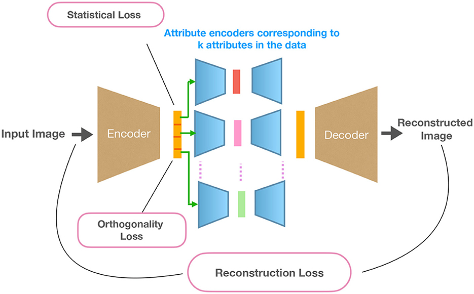
Figure 1. Overview of the proposed approach DAE-OG. Images are transformed with an encoder to a low-dimensional latent space. This representation is partitioned into k disjoint subparts corresponding to k attributes and transformed by k attribute auto-encoders. This is followed by a decoder that reconstructs the image from the concatenated attribute auto-encoder representations.

Our approach first embeds the training images into a low-dimensional representation followed by mapping disjoint parts of these representations to low-dimensional latent vectors with attribute auto-encoders, aiming to encode different attributes in the data. This is followed by a decoder/generator network that transforms representations from attribute auto-encoders to an image.

3.1 Encoder network

Specifically, as the first step, images are transformed by the encoder e(θ) to the latent representation ${\text{z}}_e\in {ℝ}^{n_{out}}$. The latent representation is partitioned into k equally sized subsets, where k denotes the number of distinct attributes in the data. The partitioned representations are transformed using k different attribute auto-encoders.

3.2 Relevance of attribute auto-encoders

Specifically, we utilize attribute encoder networks that transform a disjoint subset of latent representations further into a lower dimension space. This allows the network to learn, from disjoint latent dimensions, relevant and informative factors of variations that control different aspects of the image. The choice of the number of such attribute auto-encoders is empirically based on observed factors of variations in the data. This is also based on the assumption that the images are created by different factors that can vary independently of each other, which is often the case in practical situations. Each of the attribute auto-encoder transforms the subset of latent representation to an integral latent representation of dimension n_k for the k^th attribute. We choose n_k as the number of unique variations in an attribute.

3.3 Decoder network

The decoder network is responsible for reconstructing an image of the same size as the input using the embeddings from the attribute encoders. The embeddings are stacked in-order and fed to the decoder network for reconstruction. For the sake of simplicity, we refer to the combined parameters of attribute encoders and the decoder network as ϕ and the mapping function as g.

3.4 Loss Functions

We now present details of our loss functions that enable disentangled representation learning in an auto-encoder framework. Our loss function consists of three parts that are discussed below:

3.4.1 Reconstruction loss

Given an autoencoder, reconstruction loss measures the ability of the network to reconstruct an image from the input image when transformed into a low-dimensional space.

3.4.2 Enforcing orthogonality on latent embeddings

We impose the orthogonality constraint on the initial latent space. To achieve disentangled representation, we enforce orthogonality constraint on representations of every image. The encoder transforms the image to n_out dimensions. In order to ensure stability during network training, the subset dimensions are normalized to unity, as given by Equation (1).

3.4.3 Enforcing ${\mathcal{L}}_{stat}$ on latent embeddings

Given an unknown target distribution, the main objective was to learn an implicit generative model where one can sample from without the ability to evaluate the distribution. This can be achieved by minimizing a divergence loss that measures the difference between the target distribution and a transformation on the latent space and can be captured by enforcing the ${\mathcal{L}}_{stat}$ on the initial latent embeddings, as given by Equation (5).

The total loss function is given as follows:

$\begin{array}{l}ℒ(\theta ,\varphi )={\text{argmin}}_{\theta ,\varphi }\Vert X-X_{recon}{\Vert }_2+{\alpha }_1\Vert Z{Z}^{\top }-I{\Vert }_2\\ +{\alpha }_2{ℒ}_{stat}(X,g(\mathcal{N}))\\ \text{ where, }Z\in {ℝ}^{n_{out}}=[{\widehat{z}}^1,{\widehat{z}}^2,\dots {\widehat{z}}^k],X_{recon}=g(e(X,\theta ),\varphi )\\ \text{ and }{\widehat{z}}^i=z^i/\Vert z^i{\Vert }_2\text{ for }i=1,2,\mathrm{..}k& (6)\end{array}$

here z^k represents the latent space representation corresponding to the k^th encoder and α₁ and α₂ are hyperparameters for the weights corresponding to the two loss functions. Here, we use θ to denote the encoder e parameters, and ϕ denotes the combined parameters of the attribute auto-encoders and the decoder for simplicity.

3.4.4 Generation

In order to generate new samples, we sample from a Gaussian prior with zero mean and unit standard deviation. The normal distribution is defined in the n_out dimensional space.

4 Experimental setup and results

In this section, we present details about the experiments to evaluate the effectiveness of our approach. Our approach is termed Disentangled Attribute Encoder with Orthogonality and Graph divergence—DAE-OG. We compare our approach DAE-OG with the model without orthogonality constraint, referred to as DAE-G.

4.1 Setup

4.1.1 Dataset description

Our approach is evaluated on the 3D shapes dataset Burgess and Kim (2018). This dataset consists of 3D shapes, procedurally generated from six ground truth independent latent factors. These factors are floor color, wall color, object color, scale, shape, and orientation. For our experiments, we re-sample the dataset to have five variations for two different objects with fixed floor hue.

4.1.2 Model

We implement the initial encoder with convolution layers followed by a fully connected layer. Each of the attribute encoders consists of FC and ELU layers. The decoder is constructed in the same way as the encoder. For our experiments, we report results with three and five attribute auto-encoders. We use the same network architecture across all our experiments–an overview of the architecture is shown in Table 1.

Table 1

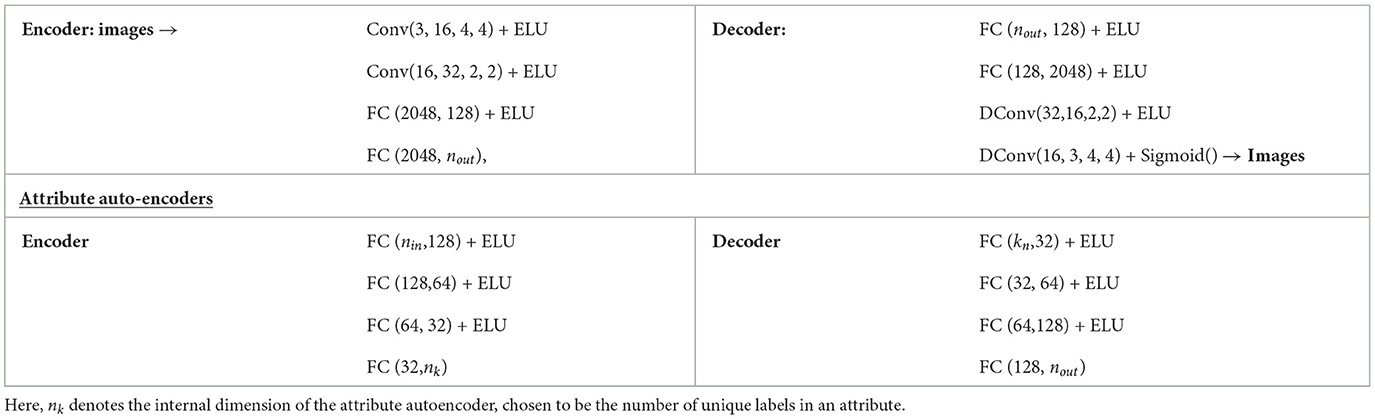
Table 1. Details of the network architectures used to design the generative model used across different experiments.

4.1.3 Training details

We adopt an annealing strategy for network training with the loss function given in Equation (6). The models are trained for 1,000 epochs, with an initial learning rate of 3e−4. The value of hyperparameters α₁ and α₂ are selected as α₁ = α₂ = 0.1 and α₁ = α₂ = 0.001 for 3 and 5 attribute spaces, respectively. We set n_out to 96 and 105 for 3 and 5 attribute encoders, respectively. In case of 3 attribute encoder network, the n_k corresponding to three attribute encoders are 6, 9, and 5. In addition, in case of 5 attribute encoder network, the n_k corresponding to the five attribute encoders are 15, 8 10, 10, and 2. For the graph divergence loss, we use k = 1 in k-nn test and λ = 0.1 for all our experiments.

4.2 Results

We compare the advantages of our model from both qualitative and quantitative aspects, across many criteria including reconstruction error, image quality, disentanglement measures, and FID scores.

4.2.1 Reconstruction fidelity

We first evaluate the reconstruction fidelity of the model both quantitatively and qualitatively. Few example images as well as corresponding reconstructed images are shown in Figure 2 for 3 and 5 partitions of the latent space. We also report MSE in Table 2. We observe that our approach consistently results in better reconstruction quality both quantitatively and qualitatively.

Figure 2

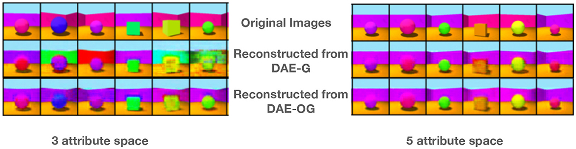
Figure 2. Some example images and the corresponding reconstructions from our proposed model DAE-OG and its improvement over DAE-G for three and five attribute spaces. DAE-OG results in better visual quality.

Table 2

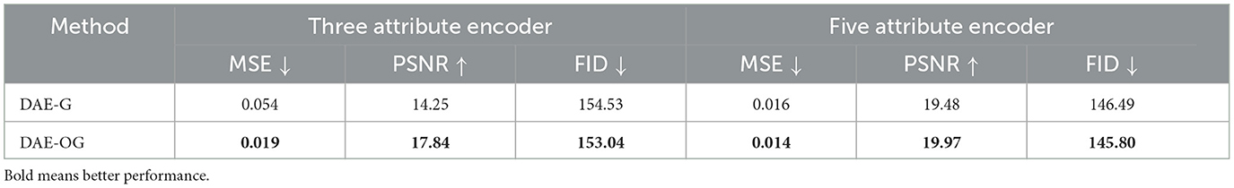
Table 2. Comparison of MSE, PSNR, and FID of DAE-G and DAE-OG models for three and five attribute encoder models.

4.2.2 Image generation

Images are generated by sampling from a normal distribution in the initial encoder latent space. Example images are shown in Figure 3 for 3 and 5 attribute encoders. We observe that DAE-OG generates images that are visibly consistently better than DAE-G.

Figure 3

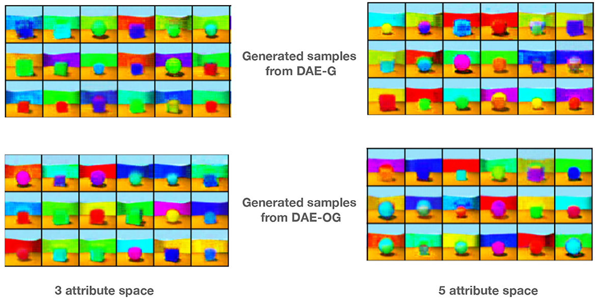
Figure 3. Some example images generated from our proposed model with three and five attribute auto-encoders by using implicit sampling for DAE-G and DAE-OG models.

4.2.3 Latent space interpolation

Latent space manipulation is important for assessing the performance of disentangling abilities of models in terms of capturing independent and semantically meaningful factors of variations. We show results by interpolating between two images in the latent space of the initial encoder. The results show that traversal in the latent space leads to smoother interpolation in the image space as well. Specifically, owing to the orthogonality constraint, we obtain better results as shown in the Figures 4–7.

Figure 4

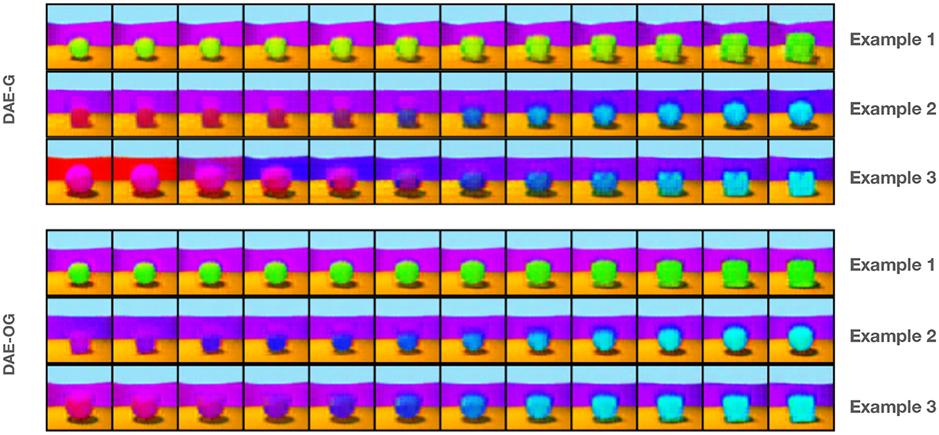
Figure 4. Three example interpolation results in the latent space of three attribute encoders on DAE-G and DAE-OG (bottom row). DAE-OG achieves a smoother interpolation.

Figure 5

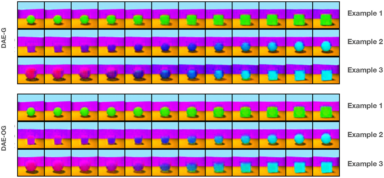
Figure 5. Three example interpolation results in the latent space of five attribute encoder. The first and the last image in each row denotes the start and end of the interpolation.

Figure 6

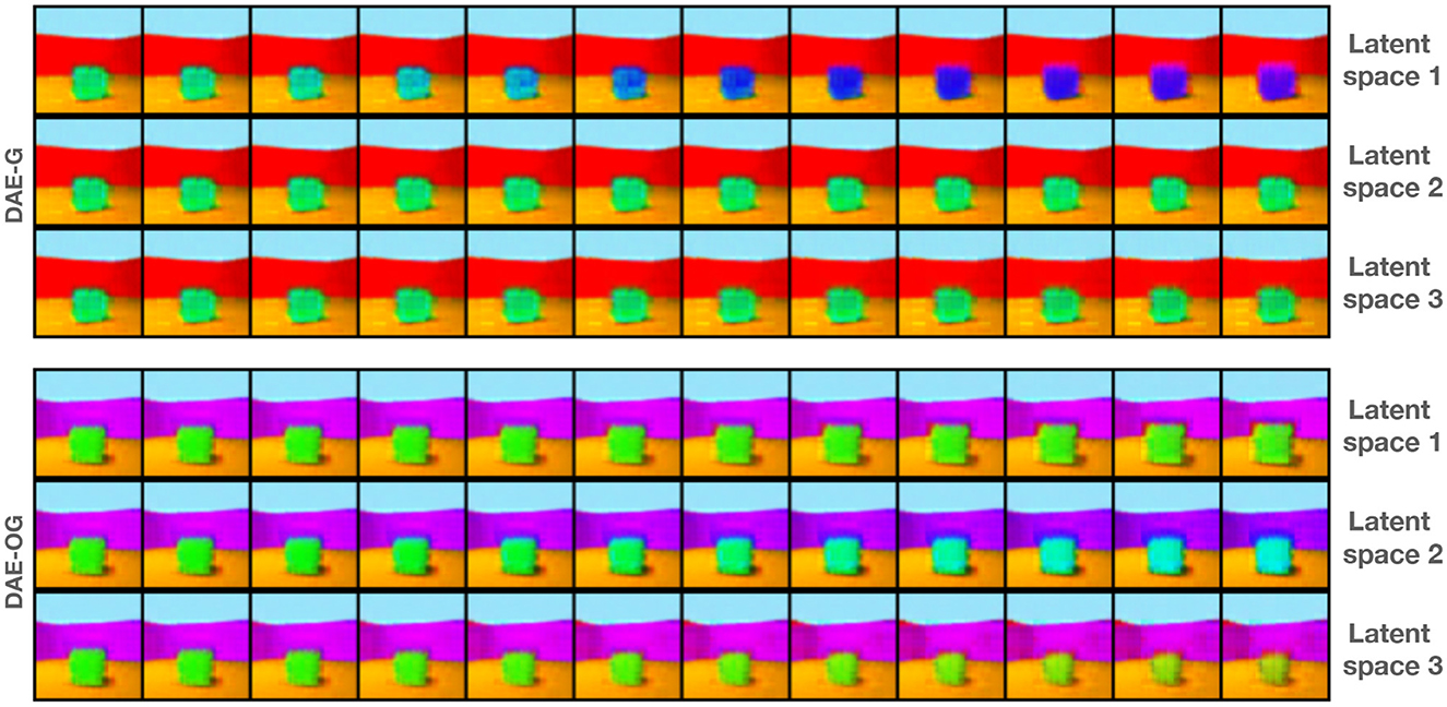
Figure 6. Interpolation along individual attribute space by keeping the other two attribute spaces frozen for a three attribute encoder-based model. For DAE-OG, in 1^st attribute space, we see variation in the size; in 2^nd attribute space, we see variation in the color of the object; and in 3^rd attribute space, we see variation in shape.

Figure 7

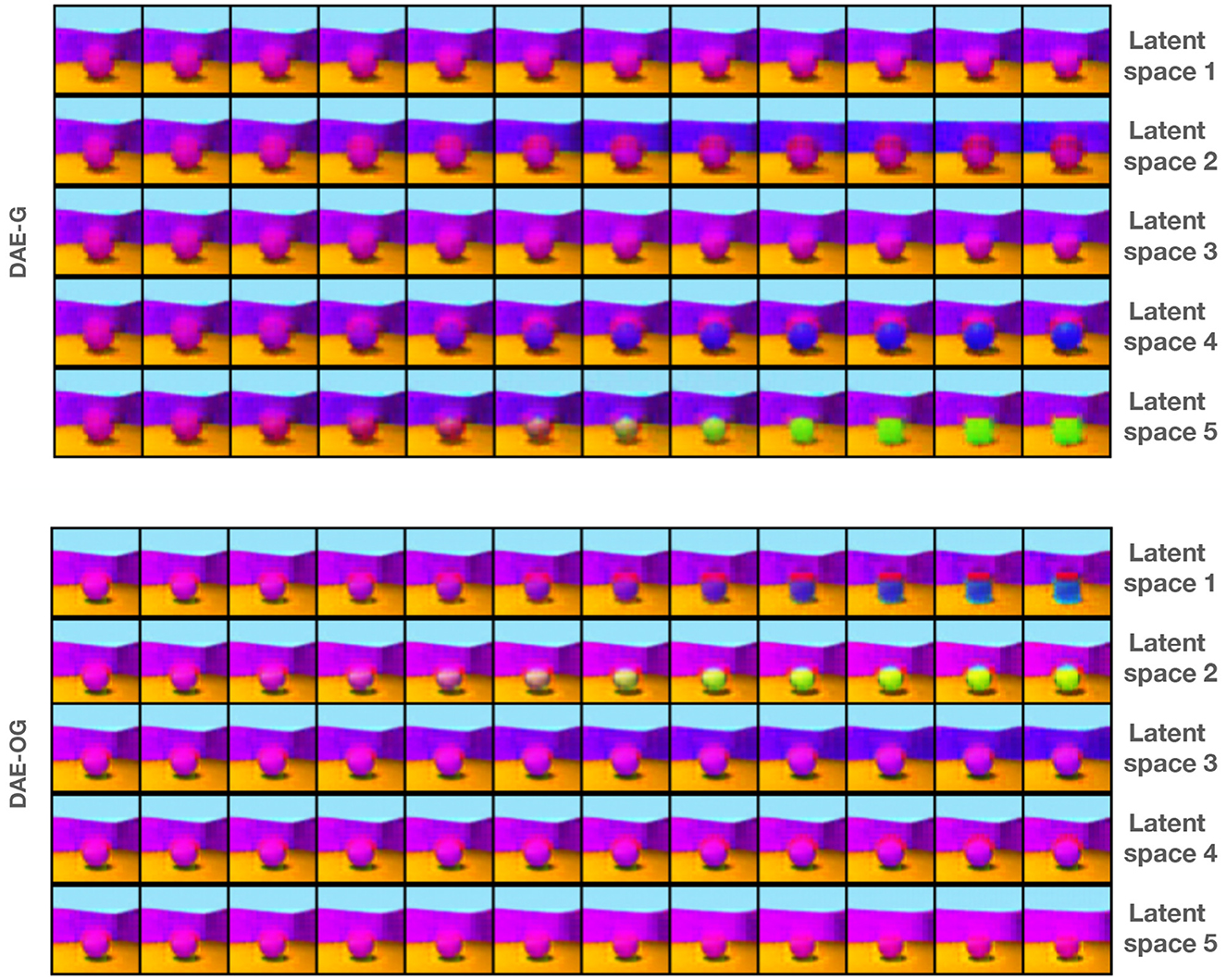
Figure 7. Interpolation along individual attribute space by keeping the other two attribute representations frozen for five attribute encoder-based model for DAE-G and DAE-OG. DAE-OG results in smoother interpolation in each space, with only one attribute change in a given space.

4.2.4 Disentanglement and FID scores

A large number of disentanglement scores have been proposed over the last several years that measure different aspects of disentanglement. We use a few of them in this study to evaluate the quality of disentanglement achieved owing to the contribution of orthogonality constraint. The results are shown in Table 3. We observe that the results with orthogonality constraints are consistently better than their counterpart.

Table 3

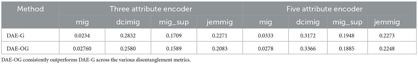
Table 3. Disentanglement metric score.

4.2.5 Effect of orthogonality

As with the method DAE-OG, we observe smoother transition within an attribute space. We note that imposing the orthogonality loss term promotes disentanglement as seen in the low-dimensional visualization of the latent space in Figure 8, done via t-SNE (van der Maaten and Hinton, 2008).

Figure 8

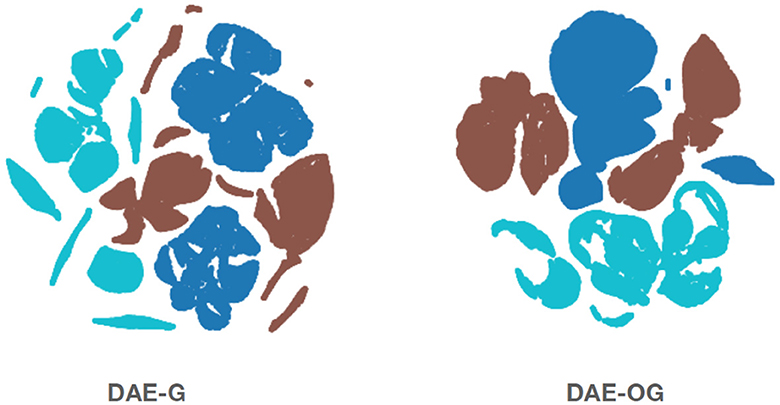
Figure 8. Two-dimensional visualization of the latent space representations showing the effect of orthogonality on the latent space representation for three attribute latent spaces. Attributes are color-coded. We note that DAE-OG achieves more compact and smoother transitions within an attribute space.

5 Discussion

The experimental datasets chosen here in our study use the 3D shapes dataset, which has simple objects and scenes; still has sufficient complexity owing to shape change, view change, and background changes. We do observe meaningful disentanglement of variables in this case. We do anticipate that scaling to more complex datasets is feasible and could form directions for future study. Due to the special nature of disentanglement tasks, where one needs to further provide some notion of meaning to variable disentangled, common datasets used in literature to assess disentangling models usually include datasets, which show some natural transitions. These include (a) KITTI-masks–which contain binary masks of pedestrians (Klindt et al., 2021), (b) the Natural Sprites dataset (Matthey et al., 2017), which consists of pairs of rendered sprite images with generative factors from the YouTube-VIS challenge, which we have experimented with before (Shukla et al., 2019), and (c) the 3DIdent dataset (Zimmermann et al., 2021), which contains objects rendered in 3D under differing lighting and viewing conditions.

The dataset we have chosen (Kim and Mnih, 2018) is another standard benchmark in this area, and is most similar to 3DIdent, however with simpler objects. With more complex objects as in 3DIdent, some of the observed visual variation will be due to self-shadowing and cast-shadowing, which would be an interesting avenue to explore the impact on disentanglement performance.

6 Conclusion

In this article, we presented an approach to learning disentangled representations in a generative framework. In addition to disentanglement, our approach enables diverse image generation and manipulation. We find that orthogonality in the latent space encourages disentanglement with a graph divergence loss that transforms the latent space. Our results support the hypothesis that inductive biases are crucial for learning disentangled representations. In future, we would like to explore the possibility of incorporating known attribute-specific constraints to further improve the interpretability of the disentangled representations.

Author's note

This study was carried out when AS was at Geometric Media Lab, Arizona State University.

Data availability statement

Publicly available datasets were analyzed in this study. This data can be found at: https://github.com/deepmind/3d-shapes.

Author contributions

AS: Conceptualization, Investigation, Methodology, Writing - original draft, Writing - review & editing. RD: Investigation, Writing - original draft. RS: Investigation, Writing - original draft. AR: Writing - original draft, Writing - review & editing. PS: Investigation, Writing - original draft, Writing - review & editing. GD: Writing - original draft, Writing - review & editing. VB: Investigation, Writing - original draft, Writing - review & editing. PT: Conceptualization, Investigation, Writing - original draft, Writing - review & editing.

Funding

The author(s) declare financial support was received for the research, authorship, and/or publication of this article. This study was supported by Defense Advanced Research Projects Agency (DARPA) under Agreement No. HR00112290073.

Conflict of interest

The authors declare that the research was conducted in the absence of any commercial or financial relationships that could be construed as a potential conflict of interest.

Publisher's note

All claims expressed in this article are solely those of the authors and do not necessarily represent those of their affiliated organizations, or those of the publisher, the editors and the reviewers. Any product that may be evaluated in this article, or claim that may be made by its manufacturer, is not guaranteed or endorsed by the publisher.

References

Achille, A., and Soatto, S. (2018). Emergence of invariance and disentanglement in deep representations. J. Machine Learn. Res. 19, 1947–1980. doi: 10.1109/ITA.2018.8503149

PubMed Abstract | Crossref Full Text | Google Scholar

Asim, M., Daniels, M., Leong, O., Ahmed, A., and Hand, P. (2020). “Invertible generative models for inverse problems: mitigating representation error and dataset bias,” in International Conference on Machine Learning (PMLR), 399–409.

Google Scholar

Bronstein, M. M., Bruna, J., LeCun, Y., Szlam, A., and Vandergheynst, P. (2017). Geometric deep learning: going beyond euclidean data. IEEE Sign. Process. Mag. 34, 18–42. doi: 10.1109/MSP.2017.2693418

Crossref Full Text | Google Scholar

Burgess, C., and Kim, H. (2018). 3D Shapes Dataset. Available online at: https://github.com/deepmind/3dshapes-dataset/

Google Scholar

Chakraborty, R., and Vemuri, B. C. (2015). “Recursive fréchet mean computation on the grassmannian and its applications to computer vision,” in IEEE International Conference on Computer Vision, ICCV 2015, 4229–4237.

Google Scholar

Choi, H., Som, A., and Turaga, P. K. (2020). Role of orthogonality constraints in improving properties of deep networks for image classification. CoRR abs/2009.10762. Available online at: https://arxiv.org/abs/2009.10762

Google Scholar

Djolonga, J., and Krause, A. (2017). “Learning implicit generative models using differentiable graph tests,” in Advances in Approximate Bayesian Inference NIPS Workshop. Available online at: http://www.approximateinference.org/2017/accepted/DjolongaKrause2017.pdf

Google Scholar

Georghiades, A. S., Belhumeur, P. N., and Kriegman, D. J. (2001). From few to many: illumination cone models for face recognition under variable lighting and pose. IEEE Trans. Pattern Anal. Mach. Intell. 23, 643–660. doi: 10.1109/34.927464

Crossref Full Text | Google Scholar

Goodfellow, I. J., Pouget-Abadie, J., Mirza, M., Xu, B., Warde-Farley, D., Ozair, S., et al. (2014). “Generative adversarial nets,” in Advances in Neural Information Processing Systems 27: Annual Conference on Neural Information Processing Systems 2014, December 8-13 2014, Montreal, Quebec, Canada, eds. Z. Ghahramani, M. Welling, C. Cortes, N. D. Lawrence, and K. Q. Weinberger, 2672–2680.

Google Scholar

Hoffman, J., Tzeng, E., Park, T., Zhu, J.-Y., Isola, P., Saenko, K., et al. (2018). “CYCADA: cycle-consistent adversarial domain adaptation,” in International Conference on Machine Learning (PMLR), 1989–1998.

Google Scholar

Kim, H., and Mnih, A. (2018). “Disentangling by factorising,” Proceedings of the 35th International Conference on Machine Learning, ser. Proceedings of Machine Learning Research, eds. J. Dy and A. Krause, vol. 80 (PMLR), 2649–2658. Available online at: https://proceedings.mlr.press/v80/kim18b.html

Google Scholar

Kingma, D. P., and Welling, M. (2013). Auto-encoding variational bayes. arXiv preprint arXiv:1312.6114. doi: 10.48550/arXiv.1312.6114

PubMed Abstract | Crossref Full Text | Google Scholar

Klindt, D. A., Schott, L., Sharma, Y., Ustyuzhaninov, I., Brendel, W., Bethge, M., et al. (2021). “Towards nonlinear disentanglement in natural data with temporal sparse coding,” International Conference on Learning Representations. Available online at: https://openreview.net/forum?id=EbIDjBynYJ8

Google Scholar

Lohit, S., and Turaga, P. K. (2017). “Learning invariant riemannian geometric representations using deep nets,” in IEEE International Conference on Computer Vision Workshops, ICCV Workshops 2017 (IEEE Computer Society), 1329–1338.

Google Scholar

Ma, J., Cui, P., Kuang, K., Wang, X., and Zhu, W. (2019). “Disentangled graph convolutional networks,” in International Conference on Machine Learning (PMLR), 4212–4221.

Google Scholar

Matthey, L., Higgins, I., Hassabis, D., and Lerchner, A. (2017). dsprites: Disentanglement Testing Sprites Dataset. Available online at: https://github.com/deepmind/dsprites-dataset/

Google Scholar

Nguyen, A. M., Yosinski, J., and Clune, J. (2015). “Deep neural networks are easily fooled: high confidence predictions for unrecognizable images,” in IEEE Conference on Computer Vision and Pattern Recognition (CVPR), 427–436.

Google Scholar

Pontin, J. (2018). Greedy, Brittle, Opaque, and Shallow: The Downsides to Deep Learning. Wired Magazine.

Google Scholar

Shao, H., Kumar, A., and Fletcher, P. T. (2018). “The riemannian geometry of deep generative models,” in 2018 IEEE/CVF Conference on Computer Vision and Pattern Recognition Workshops (CVPRW), 4288.

Google Scholar

Shukla, A., Bhagat, S., Uppal, S., Anand, S., and Turaga, P. K. (2019). “PrOSe: product of orthogonal spheres parameterization for disentangled representation learning,” in 30th British Machine Vision Conference 2019, BMVC 2019, Cardiff, UK, September 9-12, 2019 (BMVA Press), 88. Available online at: https://bmvc2019.org/wp-content/uploads/papers/1056-paper.pdf

Google Scholar

Turaga, P. K., and Srivastava, A. (2015). Riemannian Computing in Computer Vision, 1st Edn. Berlin: Springer Publishing Company, Incorporated.

Google Scholar

van der Maaten, L., and Hinton, G. (2008). Visualizing data using t-SNE. J. Machine Learn. Res. 9, 2579–2605. Available online at: http://jmlr.org/papers/v9/vandermaaten08a.html

Google Scholar

Wang, X., Jin, H., Zhang, A., He, X., Xu, T., and Chua, T.-S. (2020). “Disentangled graph collaborative filtering,” in Proceedings of the 43rd International ACM SIGIR Conference on Research and Development in Information Retrieval, 1001–1010.

Google Scholar

Zhang, C., Zhang, C., Zhang, M., and Kweon, I. S. (2023). Text-to-image diffusion model in generative AI: a survey. arXiv preprint arXiv:2303.07909. doi: 10.48550/arXiv.2303.07909

Crossref Full Text | Google Scholar

Zhu, J., Shen, Y., Zhao, D., and Zhou, B. (2020). “In-domain gan inversion for real image editing,” in European Conference on Computer Vision (Berlin: Springer), 592–608.

PubMed Abstract | Google Scholar

Zhu, J.-Y., Park, T., Isola, P., and Efros, A. A. (2017). “Unpaired image-to-image translation using cycle-consistent adversarial networks,” in Proceedings of the IEEE International Conference on Computer Vision, 2223–2232.

Google Scholar

Zimmermann, R. S., Sharma, Y., Schneider, S., Bethge, M., and Brendel, W. (2021). “Contrastive learning inverts the data generating process,” in Proceedings of the 38th International Conference on Machine Learning, eds. M. Meila and T. Zhang (PMLR), 12979–12990.

Google Scholar