- 1Department of Computer Science, Nagoya University, Nagoya, Japan
- 2Department of Engineering, Tokyo Denki University, Adachi, Japan
- 3Department of Physics and Astronomy, Tokyo University of Science, Noda, Japan
- 4Graduate School of Information Sciences, Tohoku University, Sendai, Japan
- 5Department of Physics, Tokyo Institute of Technology, Meguro, Japan
- 6Sigma-i Co., Ltd., Shinagawa, Japan
In this study, the maze generation using quantum annealing is proposed. We reformulate a standard algorithm to generate a maze into a specific form of a quadratic unconstrained binary optimization problem suitable for the input of the quantum annealer. To generate more difficulty mazes, we introduce an additional cost function Qupdate to increase the difficulty. The difficulty of the mazes was evaluated by the time to solve the maze of 12 human subjects. To check the efficiency of our scheme to create the maze, we investigated the time-to-solution of a quantum processing unit, classical computer, and hybrid solver. The results show that Qupdate generates difficult mazes tailored to the individual. Furthermore, it show that the quantum processing unit is more efficient at generating mazes than other solvers. Finally, we also present applications how our results could be used in the future.
1 Introduction
A combinatorial optimization problem is minimizing or maximizing their cost or objective function among many variables that take discrete values. In general, it takes time to solve the combinatorial optimization problem. To deal with many combinatorial optimization problems, we utilize generic solvers to solve them efficiently. Quantum annealing (QA) is one of the generic solvers for solving combinatorial optimization problems (Kadowaki and Nishimori, 1998) using the quantum tunneling effect. Quantum annealing is a computational technique to search for good solutions to combinatorial optimization problems by expressing the objective function and constraint time requirements of the combinatorial optimization problem by quantum annealing in terms of the energy function of the Ising model or its equivalent QUBO (Quadratic Unconstrained Binary Optimization) and manipulating the Ising model and QUBO to search for low energy states (Shu Tanaka and Seki, 2022). Various applications of QA are proposed in traffic flow optimization (Neukart et al., 2017; Hussain et al., 2020; Inoue et al., 2021), finance (Rosenberg et al., 2016; Orús et al., 2019; Venturelli and Kondratyev, 2019), logistics (Feld et al., 2019; Ding et al., 2021), manufacturing (Venturelli et al., 2016; Haba et al., 2022; Yonaga et al., 2022), preprocessing in material experiments (Tanaka et al., 2023), marketing (Nishimura et al., 2019), steel manufacturing (Yonaga et al., 2022), and decoding problems (Ide et al., 2020; Arai et al., 2021a). The model-based Bayesian optimization is also proposed in the literature (Koshikawa et al., 2021). A comparative study of quantum annealer was performed for benchmark tests to solve optimization problems (Oshiyama and Ohzeki, 2022). The quantum effect on the case with multiple optimal solutions has also been discussed (Yamamoto et al., 2020; Maruyama et al., 2021). As the environmental effect cannot be avoided, the quantum annealer is sometimes regarded as a simulator for quantum many-body dynamics (Bando et al., 2020; Bando and Nishimori, 2021; King et al., 2022). Furthermore, applications of quantum annealing as an optimization algorithm in machine learning have also been reported (Neven et al., 2012; Amin et al., 2018; Khoshaman et al., 2018; Kumar et al., 2018; OḾalley et al., 2018; Arai et al., 2021b; Sato et al., 2021; Urushibata et al., 2022; Goto and Ohzeki, 2023; Hasegawa et al., 2023). In this sense, developing the power of quantum annealing by considering hybrid use with various techniques is important, as mentioned in several previous studies (Hirama and Ohzeki, 2023; Takabayashi and Ohzeki, 2023).
In this study, we propose the generation of the maze by quantum annealing. In the application of quantum annealing to mazes, algorithms for finding the shortest path through a maze have been studied (Pakin, 2017). Automatic map generation is an indispensable technique for game production, including rogue-like games. Maze generation has been used to construct random dungeons in rogue-like games by assembling mazes (mok Bae et al., 2015). Therefore, considering maze generation as one of the rudiments of this technology, we studied maze generation using a quantum annealing machine. Several algorithms for the generation of the maze have been proposed. In this study, we focused on maze-generating algorithms. One can take the bar-tipping algorithm (Alg, 2023a), the wall-extending algorithm (Alg, 2023b), and the hunt-and-kill algorithm (Alg, 2023c).
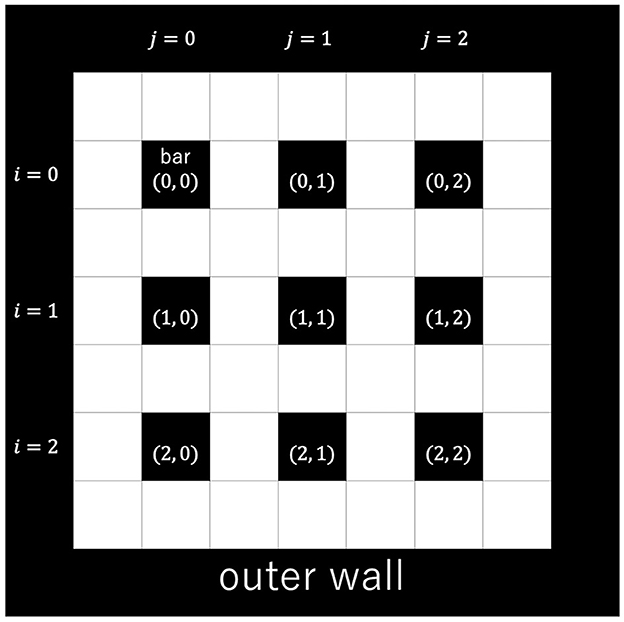
The bar-tipping algorithm is an algorithm that generates a maze by extending evenly spaced bars one by one. For the sake of explanation, we will explain the terminology here. A path represents an empty traversable part of the maze and a bar a filled non-traversable part. Figure 1 shows where the outer wall, bars, and coordinate (i, j) are in a 3 × 3 maze. The maze is surrounded by an outer wall, as shown in Figure 1. It requires the following three constraints. First, each bar can be extended by one cell only in one direction. Second, the first column can be extended in four directions: up, down, left, and right, while the second and subsequent columns can be extended only in three directions: up, down, and right. Third, adjacent bars cannot overlap each other. We explain the detailed process of the bar-tipping algorithm using the 3 × 3 size maze. In this study, a maze generated by extending the N × N bars is called N × N size maze. First, standing bars are placed in every two cells in a field surrounded by an outer wall, as shown in Figure 1. Second, Figure 2 shows each step of bar-tipping algorithm. Figure 2A shows the first column of bars extended. The bars in the first column are randomly extended in only one direction with no overlaps, as shown in Figure 2A. The bars can be extended in four directions (up, down, right, and left) at this time. Figure 2B shows the second column of bars being extended. Third, the bars in the second column are randomly extended in one direction without overlap, as shown in Figure 2B. The bars can be extended in three directions (up, down, and right) at this time. Figure 2C shows the state in which the bars after the second column are extended. Fourth, the bars in subsequent columns are randomly extended in one direction, likewise the bars in the second column, as shown in Figure 2. Figure 2D shows the complete maze in its finished state. Following the process, we can generate a maze, as shown in Figure 2D.
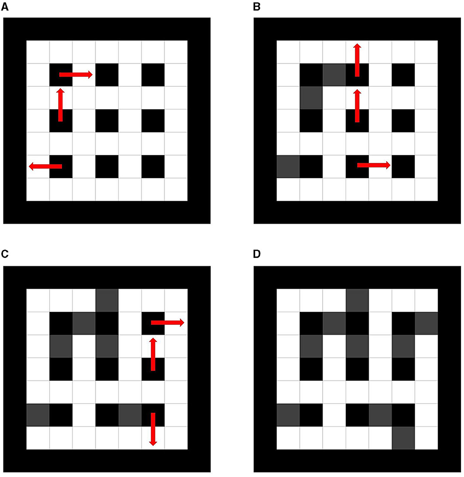
Figure 2. Step of bar-tipping algorithm. (A) Step1: bars in first column are extended. (B) Step2: bars in second column are extended. (C) Step3: bars in subsequent column are extended. (D) Step4: a complete maze through these steps.
If multiple maze solutions are possible, the maze solution is not unique, simplifying the time and difficulty of reaching the maze goal. These constraints must be followed for the reasons described below. The first constraint prevents a maze from generating a maze with multiple maze solutions and closed circuits. Figure 3A shows a maze state that violates the first constraint. The step violating the first constraint because one bar in the upper right corner is extended in two directions, as shown Figure 3A. The second constraint prevents generating a maze from a maze with closed circuits and multiple maze solutions. Figure 3B shows a state that violates the second constraint. The second constraint is violated, it has a closed circuit and multiple maze solutions, as shown in Figure 3B. The third constraint prevents maze generation from a maze with multiple maze solutions. Figure 3C shows a state that violates the third constraint. The bars overlap in the upper right corner, making it the third constraint as Figure 3C.

Figure 3. Mazes violated the constraints. (A) A maze violate the first constraint. (B) A maze violate the second constraint. (C) A maze violated the third constraint.
Next, we describe the wall-extending algorithm. It is an algorithm that generates a maze by extending walls. Figure 4 shows the extension starting coordinates of the wall-extending algorithm. Figure 5A shows the initial state of the wall-extending algorithm. First, as an initial condition, the outer perimeter of the maze is assumed to be the outer wall, and the rest of the maze is assumed to be the path, as shown in Figure 5A. Coordinate system is different from the bar-tipping algorithm, and all cells are labeled coordinates. As shown in Figure 4, the coordinates where both x and y are even and not walls are listed as starting coordinates for wall extending. The following process is repeated until all starting coordinates change to walls, as shown in Figure 5C. The coordinates were randomly chosen from the non-wall extension start coordinates. The next extending direction is randomly determined from which the adjacent cell is a path. Figure 5B shows how the path is extended. The extension will be repeated while two cells ahead of the extending direction to be extended are a path, as shown in Figure 5B. Figure 5C shows all starting coordinates changed to walls. These processes are repeated until all the starting coordinates change to walls, as shown in Figure 5C. Figure 5D shows a maze created by wall-extending. Following the process, we can generate a maze, as shown in Figure 5D.
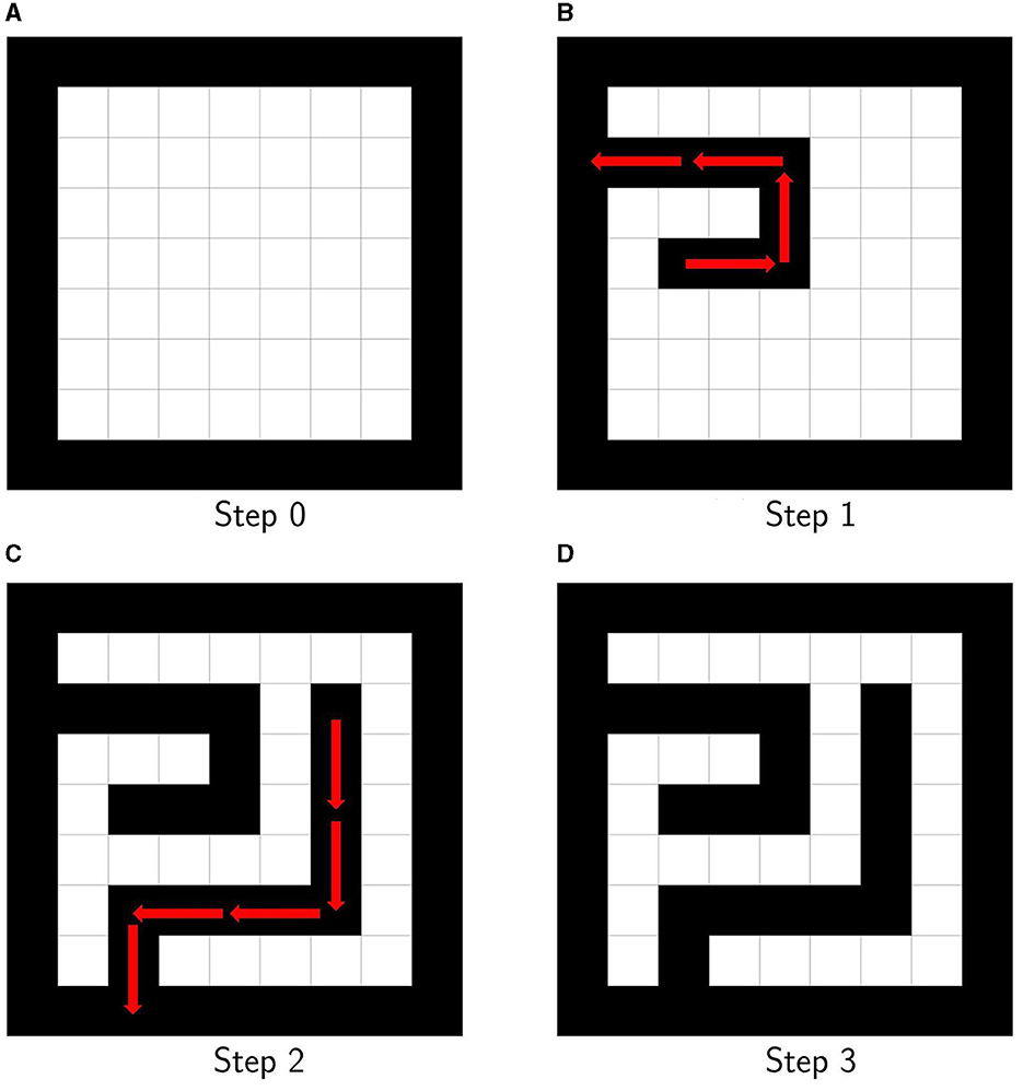
Figure 5. (A) Initial state for wall-extending algorithm. (B) Step 1 for wall-extending algorithm. (C) Step 2 for wall-extending algorithm. (D) Maze generated using wall-extending algorithm.
As a third, the hunt-and-kill algorithm is explained below. It is an algorithm that generates a maze by extending paths. Figure 6 shows the extension starting coordinates of the hunt-and-kill algorithm. Figure 7A shows the initial state of the hunt-and-kill algorithm. The entire surface is initially walled off, as shown in Figure 7A. Coordinates, where both x and y are odd, are listed as starting coordinates for path extension, as shown in Figure 6. As with the wall-extending algorithm, all cells are set to coordinates. Figure 7B shows the state in which the path is extended. A coordinate is chosen randomly from the starting coordinates, and the path is extended from there, as shown in Figure 7B. Figure 7C shows the coordinate selection and re-extension after the path can no longer be extended. If the path can no longer be extended, a coordinate is randomly selected from the starting coordinates, which are already paths, and extension starts again from it, as shown in Figure 7C. This process is repeated until all the starting coordinates turn into paths to generate the maze. Figure 7D shows the complete maze with the hunt-and-kill algorithm. Following the process, we can generate a maze, as shown in Figure 7D.
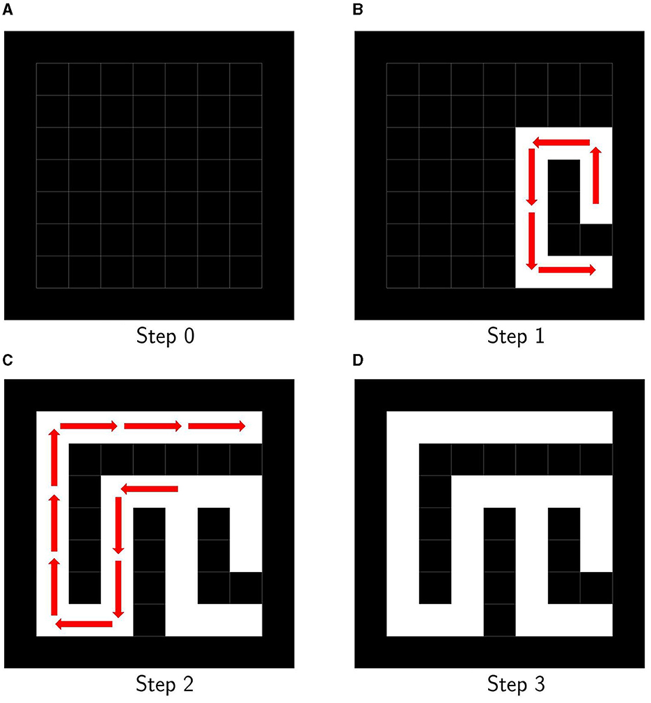
Figure 7. (A) Initial state for hunt-and-kill algorithm. (B) Step 1 for hunt-and-kill algorithm. (C) Step 2 for hunt-and-kill algorithm. (D) Maze generated using hunt-and-kill algorithm.
Of the three maze generation algorithms mentioned above, the bar-tipping algorithm is relevant to the combinatorial optimization problem. In addition, unlike other maze generation algorithms, the bar-tipping algorithm is easy to apply because it only requires the consideration of adjacent elements. Thus, we have chosen to deal with this algorithm. Other maze generation algorithms could be generalized by reformulating them as combinatorial optimization problems. The wall-extending and hunt-and-kill algorithms will be implemented in future studies, considering the following factors. The former algorithm introduces the rule that adjacent walls are extended and so are their walls. The number of connected components will be computed for the latter, and the result will be included in the optimization.
Using the bar-tipping algorithm, we reformulated it to solve a combinatorial optimization problem that generates a maze with a longer solving time and optimizes it using quantum annealing. Quantum annealing (DW_2000Q_6 from D-Wave), classical computing (simulated annealing, simulated quantum annealing, and algorithmic solution of the bar-tipping algorithm), and hybrid computing were compared with each other according to the generation time of mazes, and their performance was evaluated. The solver used in this experiment is as follows: DW_2000Q_6 from D-Wave, simulated annealer called SASampler and simulated quantum annealer called SQASampler from OpenJij (Ope, 2023), D-Wave's quantum-classical hybrid solver called hybrid_binary_quadratic_model_version2 (BQM), and classical computer [MacBook Pro(14-inch, 2021), OS: macOS Monterey Version 12.5, Chip: Apple M1 Pro, Memory: 16 GB]. This comparison showed that quantum annealing was faster. This may be because the direction of the bars is determined at once using quantum annealing, which is several times faster than the classical algorithm. We do not use an exact solver to solve the combinatorial optimization problem. We expect some diversity in the optimal solution and not only focus on the optimal solution in maze generation. Thus, we compare three solvers, which generate various optimal solutions.
In addition, we generate mazes that reflect individual characteristics, whereas existing maze generation algorithms rely on randomness and fail to incorporate other factors. In this case, we incorporated the maze solution time as one of the other factors to solve the maze. The maze solving time was defined as the time (in seconds) from the start of solving the maze to the end of solving the maze.
The study is organized as follows. In the next Section, we explain the methods of our experiments. In Section 3, we describe the results of our experiments. In Section 4, we summarize this study.
2 Methods
2.1 Cost function
To generate the maze by quantum annealer, we need to set the cost function in the quantum annealer. One of the important features of the generation of the maze is diversity. In this sense, the optimal solution is not always unique. Since it is sufficient to obtain a structure consistent with a maze, the cost function is mainly derived from the necessary constraints of a maze, as explained below. Three constraints describe the basis of the algorithm of the bar-tipping algorithm. The cost function will be converted to a QUBO matrix to use the quantum annealer. To convert the cost function to a QUBO, the cost function must be written in a quadratic form. Using the penalty method, we can convert various constraints written in a linear form into a quadratic function. The penalty method is a method to rewrite the equality constant as a quadratic function. For example, the penalty method can rewrite an equation constant x = 1 to (x−1)2. Thus, we construct the cost function for generating the maze using the bar-tipping algorithm below.
The constraints of the bar-tipping algorithm correlate with each term in the cost function as described below. The first constraint of the bar-tipping algorithm is that the bars can be extended in only one direction. It prevents making closed circuits. The second constraint of the bar-tipping algorithm is that the bars of the first column be extended randomly in four directions (up, right, down, and left), and the second and subsequent columns can be extended randomly in three directions (up, right, and down). It also prevents the creation of closed circuits. The third constraint of the bar-tipping algorithm is that adjacent bars must not overlap. Following the constraint in the bar-tipping algorithm, we can generate a maze with only one path from the start to the goal.
The cost function consists of three terms to reproduce the bar-tipping algorithm, according to the three constraints, and determine the start and goal.
where xi, j, d denotes whether the bar in i-th row, j-th column extended in direction d (up:0, right:1, down:2, left:3). When the bar in coordinate (i, j) is extended in direction, xi, j, d takes 1, otherwise takes 0. Due to the second constraint of the bar-tipping algorithm, the bars after the second column cannot be extended on the left side; only the first column has (d = 3). Furthermore, in Equation (1) depends on i, j, d, i′, j′, and d′ and is expressed as follows
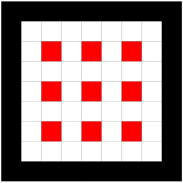
The coefficients of λ1 and λ2 are constants to adjust the effects of each penalty term. The first term prevents the bars from overlapping and extending each other face-to-face. It represents the third constraint of the bar-tipping algorithm. Here, due to the second constraint, bars in the second and subsequent columns cannot be extended to the left. Therefore, the adjacent bars in the same row cannot extend and overlap. This corresponds to the fact that d cannot take 3 when j≥1. Thus, there is no need to reflect, considering the left and right. In particular, the first term restricts the extending and overlapping between the up and down adjacent bars. For example, the situation in which one bar in (i, j) extended down (d = 2) and the lower bar in (i+1, j) extended up (d = 0) are represented by xi, j, 2xi+1, j, 0 = 1 and Q(i, j, 2), (i+1, j, 0) take 1. In the same way, thinking of the relation between the bar in (i, j) and the upper bar in (i−1, j), Q(i, j, 0), (i−1, j, 2) = 1. Thus, Q(i, j, 0), (i−1, j, 2)xi, j, 0xi−1, j, 2 takes 1, and the value of the cost function taken will increase. By doing this, the third constraint is represented as a first term. The second term is a penalty term that limits the direction of extending to one per bar. It represents the first constraint of the bar-tipping algorithm. This means that for a given coordinate (i, j), the sum of xi, j, d [d = 0, 1, 2(, 3)] must take the value 1. Here, the bars in the second and subsequent columns cannot extend to the left by the second constraint. Thus, d takes (0, 1, 2, 3) when j = 0, and d takes (0, 1, 2) when j≥1. The third term is the penalty term for selecting two coordinates of the start and the goal from the coordinates (m, n). This means that for a given coordinate (m, n), the sum of Xm, n takes 2. In other words, two coordinates were selected as the start and the goal. The start and the goal are commutative in the maze. They are randomly selected from the two coordinates determined by the third term. Xm, n denotes whether or not to set the start and goal at the m-th row and n-th column of options of start and goal coordinates. When the (m, n) coordinate is chosen as the start and goal, Xm, n takes 1. Otherwise, it takes 0. There are no relations between Xm, n and xi, j, d in Equation (1). This means that the maze structure and the start and goal determination coordinates have no relations. Figure 8 shows the coordinates (m, n) that are the options of the start and the goal. As Figure 8 shows, (m, n) is different from the coordinate setting bars; it is located at the four corners of the bars, where the bars do not extend. Xm, n and xi, j, d are different. Xm, n are options of start and goal, and xi, j, d are options of coordinates and directions to extend the bars. We have shown the simplest implementation of the maze generation following the bar-tipping algorithm by quantum annealer. Following the above a maze depending on randomness is generated. To generate a unique maze independent of randomness, we add the effect to make the maze more difficult in the cost function, and the difficulty is defined in terms of time (in seconds).
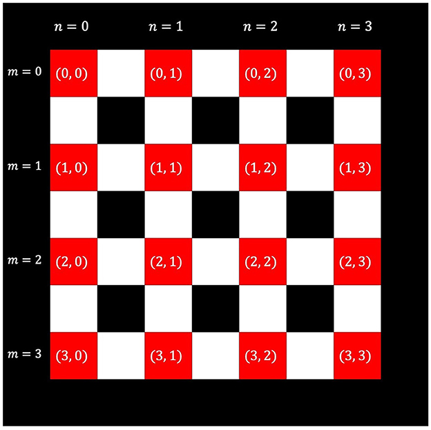
Figure 8. Black cells represent outer walls and inner bars (i, j). Red cells represent options of start and goal coordinates (m, n).
2.2 Update rule
We propose an additional Qupdate term to increase the time to solve the maze. We introduce a random term that takes random elements to change the maze structure. It is added to the Equation (1). First, Qupdate term, the additional term which includes the new QUBO matrix Qupdate, is given by
where
Figure 9 shows the structure of Qupdate and roles. Here, k′, l′ are the replacement of i, j, m, n, and d in k, l with i′, j′, m′, n′, and d′. N in Equation (4) is the size of the maze. The coefficients λupdate1 and λupdate2 are constants to adjust the effect of terms. The elements of Qupdate related to the relation between the start and goal determination and the maze generation. This is located in part B, C in Figure 9 and multiplied by the λupdate1. The elements of Qupdate related to the relation between the start and goal determination and the maze generation, part B, C in Figure 9 is multiplied by the λupdate1. The elements of Qupdate related to the start and goal determination, part D in Figure 9 is multiplied by the λupdate2. These are to control the maze difficulty without breaking the bar-tipping algorithm's constraints. Equation (3) is represented by the serial number k of each coordinate (i, j) at which bars can extend, and the sum l of the total number of coordinates at which the bars can extend and the serial number of coordinates (m, n), which are options for the start and the goal. Furthermore, The second term and the third term in Equation (3) allow the maze to consider the relation between the structure of the maze and the coordinates of the start and the goal.
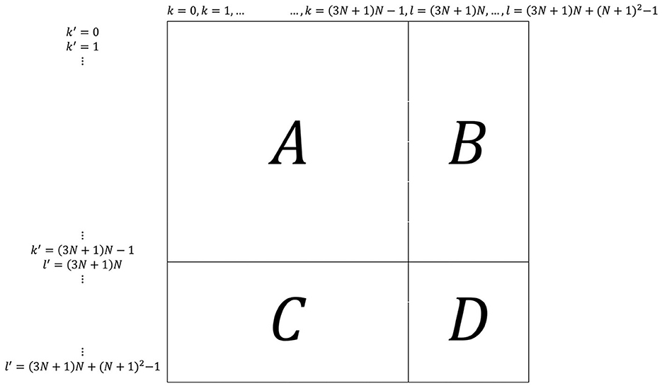
Figure 9. Structure of Qupdate. Part A is related to maze generation. Part B and part C are related to the relation between maze generation and the start and goal determination. Part D is related to the start and goal determination.
Second, Qupdate, the new QUBO matrix, is given by
where Qrandom is a matrix of random elements from −1 to 1 and p(t) depends on time t (in seconds) taken to solve the previous maze and is expressed as follows:
The Qupdate is a matrix that was made with the aim of increasing the maze solving time through the maze solving iteration. The initial Qupdate used in the first maze generation is a random matrix, and the next Qupdate that is used in the second or subsequent maze generation is updated using Equation (5), the maze solving time t, and the previous Qupdate. The longer the solving time t of the maze is, the higher the percentage of the previous Qupdate in the current Qupdate and the lower the percentage of Qrandom; inversely, when t is small, the ratio of the previous Qupdate is small, and the percentage of Qrandom is significant. In other words, the longer the solving time t of the previous maze, the more characteristics of the previous term Qupdate remain. Here, a is a constant to adjust the percentage. The p(t) is a function that increases monotonically with t and takes 0 to 1. Thus, Qrandom, which the random element in Qupdate, increase as time t increases. After the maze is solved, the next maze QUBO is updated by Equation (5) using the time taken to solve the maze. The update is carried out only once before the maze generation. Repetition of the update will make the maze gradually difficult for individuals.
The sum of Equations (1) and (3) is always used to generate a new maze annealing from a maximally mixed state.
2.3 Experiments
2.3.1 Generation of maze
We generate mazes by optimizing the cost function using DW_2000Q_6. Since the generated maze will not be solved, the update term is excluded for this experiment. λ1 = 2 and λ2 = 2 were chosen.
2.3.2 Computational cost
We compare the generation times of N × N maze in DW_2000Q_6 from D-Wave, simulated annealer called SASampler and simulated quantum annealer called SQASampler from OpenJij, D-Wave's quantum-classical hybrid solver called hybrid_binary_quadratic_model_version2 (hereinafter referred to as “Hybrid Solver”) and classical computer [MacBook Pro(14-inch, 2021), OS: macOS Monterey Version 12.5, Chip: Apple M1 Pro, Memory: 16 GB] based on bar-tipping algorithm coded with Python 3.11.5 (hereinafter referred to as “Classic”). The update term was excluded from this experiment. We set λ1 = 2 and λ2 = 2. DW_2000Q_6 was annealed 1,000 times for 20 μs, and its QPU annealed time for maze generation as calculated using time-to-solution (TTS). SASampler and SQASampler were annealed with 1,000 sweeps. These parameters were constant throughout this experiment. Regression curves fitted using the least squares method were drawn from the results to examine the dependence of computation time on maze size.
2.3.3 Effect of update term
The solving time of 9 × 9 maze generated without Qupdate and using Qupdate was measured. This experiment asked 12 human subjects to solve mazes one set (30 times). To prevent the players from memorizing maze structure, they can only observe the limited 5 × 5 cells. In other words, only two surrounding cells can be observed. The increase rate from the first step of simple moving average of 10 solving times was plotted on the graph. For this experiment, λ1 = 2, λ2 = 2, λupdate1 = 0.15, λupdate2 = 0.30, and a = 0.05 were chosen. For two λupdate, we chose larger values that do not violate the constraints of the bar-tipping algorithm. We chose a value in which Equation (6) will be ~0.8 (80%) when t = 30 s as a constant a.
2.4 Applicatons
The cost function in this study has many potential applications by generalizing it. For example, it can be applied to graph coloring and traffic light optimization. Graph coloring can be applied by allowing adjacent nodes to have different colors. Traffic light optimization can address the traffic light optimization problem by looking at the maze generation as traffic flow. Roughly speaking, our cost function can be applied to the problem of determining the next state by looking at adjacent states.
Qupdate can be applied to the problem of determining the difficulty of the next state from the previous result. The selection of personalized educational materials is one of the examples. Based on the solving time of the previously solved problems, the educational materials can be selected at a difficulty suitable for the individual. This is the most fascinating direction in future studies. As described above, we should emphasize that Qupdate proposed in this study also has potential use in various fields related to training and education.
3 Results
3.1 Generation of maze
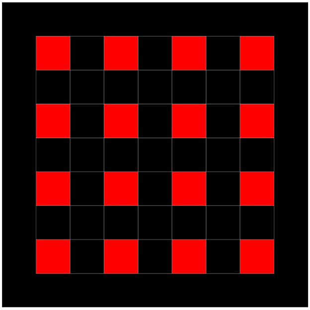
Figure 10 shows execution examples of 9 × 9 and 15 × 15 mazes generated by optimizing the cost function using DW_2000Q_6.
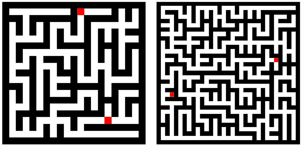
Figure 10. (Left) 9 × 9 maze generated by DW_2000Q_6. (Right) 15 × 15 maze generated by DW_2000Q_6. Red cells represent a start and a goal for the maze.
3.2 Computational cost
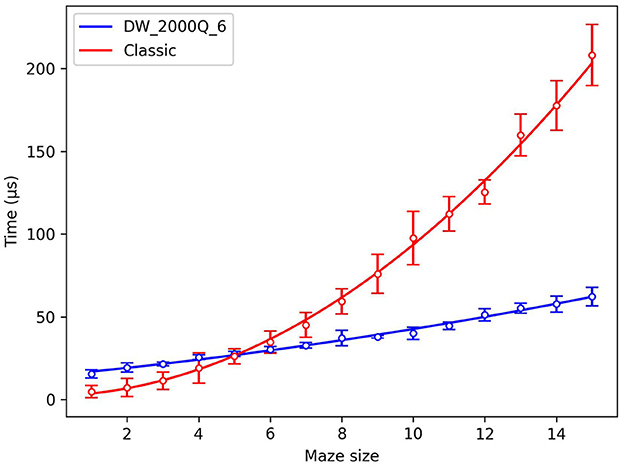
Fits of the form aN2+bN+c is applied to each of the datasets using the least squares method. The results are as follows. Figure 11 shows the relation between TTS for maze generation and maze size on DW_2000Q_6. DW_2000Q_6 is or . Even if it is quadratically dependent on the maze size, its deviation is smaller than the other solvers. Figure 12 shows the relation between maze generation time and maze size on Classic, SASampler, and SQASampler. Classic [(0.855 ± 0.090)N2+(0.6 ± 1.5)N+(2.2 ± 5.1)], SASampler [(28.8 ± 1.2)N2+(36 ± 20)N+(129 ± 71)], and SQASampler [(172.8 ± 4.4)N2+(287 ± 73)N−(1.5 ± 2.5)·102] exhibit quadratic dependence on the maze size . Most of the solvers introduced here are since they are extending N × N bars to generate a maze. Figure 13 shows the comparison of maze generation time between DW_2000Q_6 and Classic. DW_2000Q_6 has a smaller coefficient N2 than the classical algorithm, and after N = 5, DW_2000Q_6 shows an advantage over Classic in the maze generation problem. The improvement using quantum annealing occurred because it determines the direction of N × N bars at once. Figure 14 shows the relation between maze generation time and maze size on Hybrid Solver. Linear and quadratic fits applied to the dataset indicate that the Hybrid Solver is or [(3.29 ± 0.83)·102N+(2.99325 ± 0.00090)·106] between N = 1 and N = 18 and then shifted to [(6.899 ± 0.065)·103N2−(0.4 ± 3.2)·103N+(6.90 ± 0.39)·105]. The shift in the computational cost of Hybrid Solver may have resulted from a change in its algorithm.
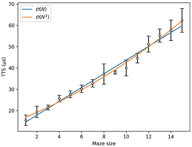
Figure 11. Time to reach the ground state with 99% success probability as a function of the maze size in DW_2000Q_6. The error bars represent a 95% confidence interval. The regression curve is given by [(3.231 ± 0.076)N + (11.40 ± 0.69)] for linear regression and [(7.4 ± 1.8) · 10−2N2 + (2.05 ± 0.30)N + (14.8 ± 1.0)] for quadratic regression.

Figure 12. (A) The time to reach the ground state as a function of the maze size in Classic. The error bars represent a 95% confidence interval. The regression curve is [(0.855 ± 0.090)N2 + (0.6 ± 1.5)N + (2.2 ± 5.1)]. (B) Time to reach the ground state as a function of the maze size in SASampler. The error bars represent a 95% confidence interval. The regression curve is [(28.8 ± 1.2)N2 + (36 ± 20)N + (129 ± 71)]. (C) Time to reach the ground state as a function of the maze size in SQASampler. The error bars represent a 95% confidence interval. The regression curve is [(172.8 ± 4.4)N2 + (287 ± 73)N −(1.5 ± 2.5) · 102].
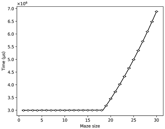
Figure 14. Time to reach the ground state as a function of maze size in the Hybrid Solver. The error bars represent a 95% confidence interval.
3.3 Effect of update term
Here, 12 human subjects are asked to solve the maze one set (30 times), and the maze is shown to increase in difficulty as it adapts to each human subject. Figure 15A shows the increase rate from the first step of simple moving average of 10 solving time of maze generated without Qupdate and individual increase rate. The solving time of the maze without Qupdate was slightly getting shorter overall. Figure 15B shows the increase rate from the first step of simple moving average of 10 solving time of maze generated using Qupdate and individual increase rate. The solving time of the maze using Qupdate was getting longer overall. Most of the players increased their solving time, but some players decreased or did not change their solving time. In addition, nine players' average of the solving time of the maze generated using Qupdate increased than that of the maze generated without Qupdate. These show that Qupdate has the potential to increase the difficulty of the mazes.
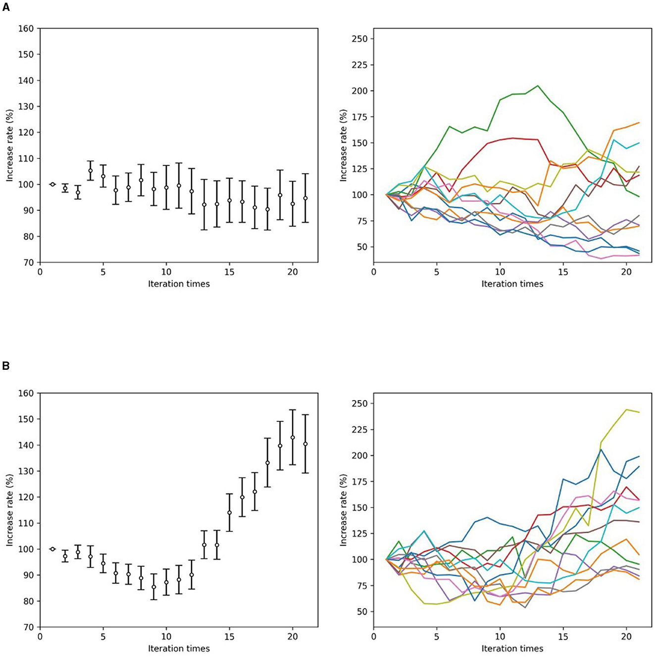
Figure 15. (A) Left: Increase rate from the first step of simple moving average of 10 solving time of 9 × 9 maze generated without Qupdate. The error bars represent standard errors. Right: All players' increase rate from the first step of simple moving average of 10 solving time of 9 × 9 maze generated without Qupdate. (B) Left: Increase rate from the first step of simple moving average of 10 solving time of 9 × 9 maze generated using Qupdate. The error bars represent standard errors. Right: All players' increase rate from the first step of simple moving average of 10 solving time of 9 × 9 maze generated using Qupdate.
4 Discussion
In this study, we show that generating difficult (longer the maze solving time) mazes using the bar-tipping algorithm is also possible with quantum annealing. By reformulating the bar-tipping algorithm as the combinatorial optimization problem, we generalize it more flexibly to generate mazes. In particular, our approach is simple but can adjust the difficulty in solving mazes by quantum annealing.
In Section 3.2, regarding comparing computational costs to solve our approach to generating mazes using TTS, DW_2000Q_6 has a smaller coefficient of N2 than the classical counterpart. Therefore, as N increases, the computational cost of DW_2000Q_6 can be expected to be lower than that of the classical simulated annealing for a certain time. Unfortunately, since the number of qubits in the D-Wave quantum annealer is finite, the potential power of generating mazes by quantum annealing is limited. However, our insight demonstrates some advantages of quantum annealing against its classical counterpart. In addition, we observed that the hybrid solver's computational cost was constant up to N = 18. This indicates that hybrid solvers will be potentially effective if they are developed to deal with many variables in future.
In Section 3.3, we proposed Qupdate to increase the solving time using quantum annealing. We demonstrated that introducing Qupdate increased the time to solve the maze and changed the difficulty compared with the case where Qupdate was not introduced. At this time, the parameters (λupdate1, λupdate2, and a) were fixed. Difficult maze generation for everyone may be possible by adjusting the parameters individually.
One of the directions in the future study is in applications of our cost function in various realms. We should emphasize that Qupdate proposed in this study also has the potential use in various fields related to training and education. The powerful computation of quantum annealing and its variants open the way to such realms with high-speed computation and various solutions.
Data availability statement
The original contributions presented in the study are included in the article/supplementary material, further inquiries can be directed to the corresponding authors.
Ethics statement
Ethical approval was not required for the studies involving humans because the data was obtained through collaboration among the participants of a group workshop developing an application using quantum annealing. The studies were conducted in accordance with the local legislation and institutional requirements. Written informed consent for participation was not required from the participants or the participants' legal guardians/next of kin in accordance with the national legislation and institutional requirements because the data was obtained through collaboration among the participants of a group workshop developing an application using quantum annealing.
Author contributions
YI: Writing – original draft, Writing – review & editing, Conceptualization, Data curation, Formal analysis, Investigation, Software, Validation, Visualization, Methodology. TY: Writing – original draft, Writing – review & editing, Conceptualization, Validation, Methodology. KO: Writing – original draft, Writing – review & editing, Conceptualization, Validation, Methodology. MO: Supervision, Writing – review & editing, Funding acquisition, Project administration.
Funding
The author(s) declare financial support was received for the research, authorship, and/or publication of this article. The authors thank financial support from the MEXT-Quantum Leap Flagship Program Grant No. JPMXS0120352009, as well as Public\Private R&D Investment Strategic Expansion PrograM (PRISM) and programs for Bridging the gap between R&D and the IDeal society (society 5.0) and Generating Economic and social value (BRIDGE) from Cabinet Office.
Acknowledgments
The authors thank the fruitful discussion with Reo Shikanai and Yoshihiko Nishikawa on applications of our approach to another application. This study is the result of research developed from an exercise class held at Tohoku University in Japan in the past called Quantum Annealing for You, 2nd party!. We want to thank one of the supporters, Rumiko Honda, for supporting the operations. The participants were a diverse group, ranging from high school students to university students, graduate students, technical college students, and working adults. As we can see from the authors' affiliations, this is a good example of a leap from the diversity of the participants to the creation of academic and advanced content.
Conflict of interest
MO is employed by Sigma-i.
The remaining authors declare that the research was conducted without any commercial or financial relationships that could be construed as a potential conflict of interest.
Publisher's note
All claims expressed in this article are solely those of the authors and do not necessarily represent those of their affiliated organizations, or those of the publisher, the editors and the reviewers. Any product that may be evaluated in this article, or claim that may be made by its manufacturer, is not guaranteed or endorsed by the publisher.
References
Alg (2023a). Available online at:https://algoful.com/Archive/Algorithm/MazeBar (accessed August 13, 2023).
Alg (2023b). Available online at: https://algoful.com/Archive/Algorithm/MazeExtend (accessed August 13, 2023).
Alg (2023c). Available online at: https://algoful.com/Archive/Algorithm/MazeDig (accessed August 13, 2023).
Amin, M. H., Andriyash, E., Rolfe, J., Kulchytskyy, B., and Melko, R. (2018). Quantum Boltzmann machine. Phys. Rev. X, 8. doi: 10.1103/PhysRevX.8.021050
Arai, S., Ohzeki, M., and Tanaka, K. (2021a). Mean field analysis of reverse annealing for code-division multiple-access multiuser detection. Phys. Rev. Res. 3, 033006. doi: 10.1103/PhysRevResearch.3.033006
Arai, S., Ohzeki, M., and Tanaka, K. (2021b). Teacher-student learning for a binary perceptron with quantum fluctuations. J. Phys. Soc. Jpn. 90, 074002. doi: 10.7566/JPSJ.90.074002
Bando, Y., and Nishimori, H. (2021). Simulated quantum annealing as a simulator of nonequilibrium quantum dynamics. Phys. Rev. A 104, 022607. doi: 10.1103/PhysRevA.104.022607
Bando, Y., Susa, Y., Oshiyama, H., Shibata, N., Ohzeki, M., Gömez-Ruiz, F. J., et al. (2020). Probing the universality of topological defect formation in a quantum annealer: Kibble-zurek mechanism and beyond. Phys. Rev. Res. 2, 033369. doi: 10.1103/PhysRevResearch.2.033369
Ding, Y., Chen, X., Lamata, L., Solano, E., and Sanz, M. (2021). Implementation of a hybrid classical-quantum annealing algorithm for logistic network design. SN Comp. Sci. 2, 1–9. doi: 10.1007/s42979-021-00466-2
Feld, S., Roch, C., Gabor, T., Seidel, C., Neukart, F., Galter, I., et al. (2019). A hybrid solution method for the capacitated vehicle routing problem using a quantum annealer. Front. ICT 6, 13. doi: 10.3389/fict.2019.00013
Goto, T., and Ohzeki, M. (2023). Online calibration scheme for training restricted boltzmann machines with quantum annealing. arXiv [Preprint]. arXiv:2307.09785
Haba, R., Ohzeki, M., and Tanaka, K. (2022). Travel time optimization on multi-agv routing by reverse annealing. Sci. Rep. 12, 17753. doi: 10.1038/s41598-022-22704-0
Hasegawa, Y., Oshiyama, H., and Ohzeki, M. (2023). Kernel learning by quantum annealer. arXiv [Preprint]. arXiv:2304.10144
Hirama, S., and Ohzeki, M. (2023). Efficient algorithm for binary quadratic problem by column generation and quantum annealing. arXiv. doi: 10.7566/JPSJ.92.113002
Hussain, A., Bui, V.-H., and Kim, H.-M. (2020). Optimal sizing of battery energy storage system in a fast ev charging station considering power outages. IEEE Transact. Transport. Electr. 6, 453–463. doi: 10.1109/TTE.2020.2980744
Ide, N., Asayama, T., Ueno, H., and Ohzeki, M. (2020). “Maximum likelihood channel decoding with quantumannealingmachine,” in 2020 International Symposium on Information Theory and Its Applications (ISITA), 91–95.
Inoue, D., Okada, A., Matsumori, T., Aihara, K., and Yoshida, H. (2021). Traffic signal optimization on a square lattice with quantum annealing. Sci. Rep. 11, 1–12. doi: 10.1038/s41598-021-82740-0
Kadowaki, T., and Nishimori, H. (1998). Quantum annealing in the transverse ising model. Phys. Rev. E 58, 5355–5363. doi: 10.1103/PhysRevE.58.5355
Khoshaman, A., Vinci, W., Denis, B., Andriyash, E., Sadeghi, H., and Amin, M. H. (2018). Quantum variational autoencoder. Quant. Sci. Technol. 4, 014001. doi: 10.1088/2058-9565/aada1f
King, A. D., Suzuki, S., Raymond, J., Zucca, A., Lanting, T., Altomare, F., et al. (2022). Coherent quantum annealing in a programmable 2,000 qubit ising chain. Nat. Phys. 18, 1324–1328. doi: 10.1038/s41567-022-01741-6
Koshikawa, A. S., Ohzeki, M., Kadowaki, T., and Tanaka, K. (2021). Benchmark test of black-box optimization using d-wave quantum annealer. J. Phys. Soc. Jpn. 90, 064001. doi: 10.7566/JPSJ.90.064001
Kumar, V., Bass, G., Tomlin, C., and Dulny, J. (2018). Quantum annealing for combinatorial clustering. Quant. Inf. Process. 17, 39. doi: 10.1007/s11128-017-1809-2
Maruyama, N., Ohzeki, M., and Tanaka, K. (2021). Graph minor embedding of degenerate systems in quantum annealing. arXiv [Preprint]. arXiv:2110.10930
mok Bae, C., Kim, E. K., Lee, J., joong Kim, K., and Na, J.-C. (2015). Generation of an Arbitrary Shaped Large Maze by Assembling Mazes. New York, NY: IEEE. doi: 10.1109/CIG.2015.7317901
Neukart, F., Compostella, G., Seidel, C., Von Dollen, D., Yarkoni, S., and Parney, B. (2017). Traffic flow optimization using a quantum annealer. Front. ICT 4, 29. doi: 10.3389/fict.2017.00029
Neven, H., Denchev, V. S., Rose, G., and Macready, W. G. (2012). “Qboost: large scale classifier training withadiabatic quantum optimization,” in Asian Conference on Machine Learning (PMLR) (New York, NY), 333–348.
Nishimura, N., Tanahashi, K., Suganuma, K., Miyama, M. J., and Ohzeki, M. (2019). Item listing optimization for e-commerce websites based on diversity. Front. Comput. Sci. 1, 2. doi: 10.3389/fcomp.2019.00002
OḾalley, D., Vesselinov, V. V., Alexandrov, B. S., and Alexandrov, L. B. (2018). Nonnegative/binary matrix factorization with a d-wave quantum annealer. PLoS ONE 13, e0206653. doi: 10.1371/journal.pone.0206653
Ope (2023). Available online at: https://www.openjij.org/ (accessed October 10, 2023).
Orús, R., Mugel, S., and Lizaso, E. (2019). Forecasting financial crashes with quantum computing. Phys. Rev. A 99, 060301. doi: 10.1103/PhysRevA.99.060301
Oshiyama, H., and Ohzeki, M. (2022). Benchmark of quantum-inspired heuristic solvers for quadratic unconstrained binary optimization. Sci. Rep. 12, 2146. doi: 10.1038/s41598-022-06070-5
Pakin, S. (2017). “Navigating a maze using a quantum annealer,” in ITiCSE-WGR 2017 - Proceedings of the 2017 ITiCSE Conference onWorking Group Reports (New York, NY). doi: 10.1145/3149526.3149532
Rosenberg, G., Haghnegahdar, P., Goddard, P., Carr, P., Wu, K., and De Prado, M. L. (2016). Solving the optimal trading trajectory problem using a quantum annealer. IEEE J. Sel. Top. Signal Process. 10, 1053–1060. doi: 10.1109/JSTSP.2016.2574703
Sato, T., Ohzeki, M., and Tanaka, K. (2021). Assessment of image generation by quantum annealer. Sci. Rep. 11, 13523. doi: 10.1038/s41598-021-92295-9
Shu Tanaka, M. Y., and Seki, Y. (2022). Black-box optimization by anneling machines. J. Neural Circ. Soc. Jpn. 29, 164–173. doi: 10.3902/jnns.29.164
Takabayashi, T., and Ohzeki, M. (2023). Hybrid algorithm of linear programming relaxation and quantum annealing. arXiv [Preprint]. arXiv:2308.10765
Tanaka, T., Sako, M., Chiba, M., Lee, C., Cha, H., and Ohzeki, M. (2023). Virtual screening of chemical space based on quantum annealing. J. Phys. Soc. Jpn. 92, 023001. doi: 10.7566/JPSJ.92.023001
Urushibata, M., Ohzeki, M., and Tanaka, K. (2022). Comparing the effects of boltzmann machines as associative memory in generative adversarial networks between classical and quantum samplings. J. Phys. Soc. Jpn. 91, 074008. doi: 10.7566/JPSJ.91.074008
Venturelli, D., and Kondratyev, A. (2019). Reverse quantum annealing approach to portfolio optimization problems. Quant. Mach. Intell. 1, 17–30. doi: 10.1007/s42484-019-00001-w
Venturelli, D., Marchand, D. J. J., and Rojo, G. (2016). Quantum annealing implementation of job-shop scheduling. arXiv [Preprint]. arXiv:1506.08479
Yamamoto, M., Ohzeki, M., and Tanaka, K. (2020). Fair sampling by simulated annealing on quantum annealer. J. Phys. Soc. Jpn. 89, 025002. doi: 10.7566/JPSJ.89.025002
Keywords: quantum annealing, combinatorial optimization, maze generation, bar-tipping algorithm, time-to-solution
Citation: Ishikawa Y, Yoshihara T, Okamura K and Ohzeki M (2023) Individual subject evaluated difficulty of adjustable mazes generated using quantum annealing. Front. Comput. Sci. 5:1285962. doi: 10.3389/fcomp.2023.1285962
Received: 30 August 2023; Accepted: 09 November 2023;
Published: 07 December 2023.
Edited by:
Catherine McGeoch, D-Wave Systems, CanadaReviewed by:
Michael Hanks, Imperial College London, United KingdomJemma Bennett, University of Innsbruck, Austria
Copyright © 2023 Ishikawa, Yoshihara, Okamura and Ohzeki. This is an open-access article distributed under the terms of the Creative Commons Attribution License (CC BY). The use, distribution or reproduction in other forums is permitted, provided the original author(s) and the copyright owner(s) are credited and that the original publication in this journal is cited, in accordance with accepted academic practice. No use, distribution or reproduction is permitted which does not comply with these terms.
*Correspondence: Yuto Ishikawa, aXNoaWthd2EueXV0by5mNkBzLm1haWwubmFnb3lhLXUuYWMuanA=; Takuma Yoshihara, MjFlZjEwNkBtcy5kZW5kYWkuYWMuanA=; Keita Okamura, NjIyMzAyNEBlZC50dXMuYWMuanA=
 Yuto Ishikawa
 Takuma Yoshihara
 Keita Okamura
 Masayuki Ohzeki