 David Cruz
 Jorge Batista
- 1Institute of Systems and Robotics, Coimbra University, Coimbra, Portugal
- 2Department of Electrical and Computer Engineering, Faculty of Sciences and Technology, University of Coimbra, Coimbra, Portugal
Causal assertions stem from an asymmetric relation between some variable's causes and effects, i.e., they imply the existence of a function decomposition of a model where the effects are a function of the causes without implying that the causes are functions of the effects. In structural causal models, information is encoded in the compositions of functions that define variables because that information is used to constraint how an intervention that changes the definition of a variable influences the rest of the variables. Current probabilistic models with tractable marginalization also imply a function decomposition but with the purpose of allowing easy marginalization of variables. In this article, structural causal models are extended so that the information implicitly stored in their structure is made explicit in an input–output mapping in higher dimensional representation where we get to define the cause–effect relationships as constraints over a function space. Using the cause–effect relationships as constraints over a space of functions, the existing methodologies for handling causality with tractable probabilistic models are unified under a single framework and generalized.
1 Introduction
Probabilistic inference is a problem in the complexity class #P, and computing an approximate solution for it better than a factor of 0.5 is NP-hard (Koller and Friedman, 2009). Nevertheless, there are classes of models called tractable probabilistic model (TPM) (Darwiche, 2002; Poon and Domingos, 2011; Kisa et al., 2014; Zhang et al., 2021) (see Section 3) where computing evidence and marginal queries can be guaranteed to have a cost bounded by a polynomial in its size. They can be used to model any probability distribution defined over categorical variables, and, as expected due to the hardness of approximation of inference1, their size requirements can be exponential in the problem specification size. Inference is a subroutine in learning and approximations used when learning can have an impact on what is learned (Koller and Friedman, 2009; Poon and Domingos, 2011). Moreover, different approximate inference procedures used over a learned model can yield different results for the same queries (Koller and Friedman, 2009). Using TPM where inference is guaranteed to have a bounded cost enables the utilization of exact inference procedures for learning and usage of the learned model. In that scenario, all approximations are done when choosing the structure and size of the TPM.
While probabilistic models capture co-occurrences of events in observed environments, in causal models, it is assumed that the behavior of models can change when we choose to act on the world via an yet unmnodeled process (Pearl, 2009). An intervention on a variable changes the function that was used to define the value of that variable (Pearl, 2009). Without further assumptions on how each change in an intervened variable influences the rest of the variables, the effects of an intervention are undefined (Pearl, 2009). The growth of the space of functions that is needed to model probabilistic relations in the scenarios with interventions, in tandem with the potential disruption of parameter level dependence relationships exploited to get modern compressed TPM (Darwiche, 2022), poses challenges in tying TPM and causality while avoiding large TPM models.
Research in causality is built around the proposition that it is useful to think about causes and effects while modeling the world. The study of cause–effect relationships in models is relevant due to tools it provides to its user (Pearl, 2019). It is central in many aspects of modeling such as: (1) missing data imputation (Mohan and Pearl, 2021), (2) identifiability of parameters and learnability (Tikka et al., 2019; Xia et al., 2021), (3) transportability (Bareinboim and Pearl, 2013; Pearl and Bareinboim, 2014), or (4) out-of-distribution generalization (Jalaldoust and Bareinboim, 2023). At the core of these tools are statements about inter-dependency among variables in the presence of interventions. An effect is naturally defined as a function of its causes but not the other way around. This asymmetry, already present in structural equation modeling (SEM) described in Wright (1921), is the cornerstone of the structural causal model framework (SCMF) approach to causality advocated in Pearl (2009). A key point in this article is the expression of causality through function compositions. Under this framework, a cause–effect statement is equivalent to a statement that a function can be decomposed in a specific form. Specifically, parent–child relations exist in the function decomposition through the input–output relations. However, the existence of a function decomposition that, when exploited, allows us to correctly compute the global function does not imply its explicit use.
A structural causal model (SCM) (Pearl, 2009; Bareinboim et al., 2022) is defined as a 4-tuple where: (1) is a set of functions that is used to define “endogenous” variables in SCM in the absence of interventions on them; (2) V is a set of variables that are “endogenous” to the model by virtue of being, in the absence of interventions, defined as the outputs of functions in ; (3) U is a set of “exogenous” variables whose value determines, at an individual level, every factor of variation in functions in ; and (4) stands for a probabilistic distribution over all exogenous variables. An intervention is a replacement of a function that defines an endogenous variable in structural causal models by another, yet undefined, function whose output provides the new definition of that endogenous variable (Pearl, 2009; Bareinboim et al., 2022). This implies that exogenous variables do not characterize the uncertainty over interventions, and, in that regard, they are outside of what is (explicitly) modeled by an SCM. Nevertheless, the way they influence the set of endogenous variables is well defined in that an algorithm that takes as input and the interventions can output a new set of functions can be used to answer queries containing interventions. Therefore, some of the information in an SCM is encoded in its structure.
There are three approaches to model causality with TPM: (1) using variable elimination over a SCM to get a TPM structure (Darwiche, 2022), (2) using a transformation between a TPM and a causal Bayesian network (CBN) (Papantonis and Belle, 2020) to support cause–effect claims in a TPM, and (3) using separate parameters for each interventional case, which was used in interventional sum product network (iSPN) (Zečević et al., 2021) .
The two first approaches rely on the existence of a class of models like CBN or SCM on which causality has been studied (Pearl, 2009; Bareinboim et al., 2022). TPM research was sprung in the context of efforts to accelerate inference in Bayesian networks (Chavira and Darwiche, 2005); therefore, there is good reason to ask if compilation of CBN would provide a good way to introduce causality into TPM. In Darwiche (2022) a SCM used to describe some phenomenon is compiled into a TPM via an algorithm akin to variable elimination. Similarly to SCM, an algorithm that takes as input both the structure of the computation graph (CG) (Erikssont et al., 1998; Trapp et al., 2019; Peharz et al., 2020) of a TPM and information about interventions will adjust the CG so that queries pertaining to interventions can be answered (Darwiche, 2022). The structure of TPM is used as a source of information; therefore, not all information in the TPM [in the approach taken in Darwiche (2022)] is encoded explicitly in the input–output mapping. This limits the set of structures that can be used by the TPM to those in which the algorithm that adapts the TPM to respond to queries pertaining to interventions works as intended.
The second approach depends on the ability to transform a probabilistic distribution expressed in a sum product network (SPN) or probabilistic sentential decision diagram (PSDD) (both TPM) as a bayesian Network (BN) (Papantonis and Belle, 2020). In that work, the transformations from SPN to BN described in Zhao et al. (2015) and a transformation from PSDD into BN developed in Papantonis and Belle (2020) were used for that purpose. From the BN that is obtained, in Papantonis and Belle (2020), a set of cause effect statements regarding the initial model is discussed under the assumption that the directed acyclic graph (DAG) of the BN encodes a set of cause–effect relationships. In either the CBN, SCM, or TPM in Papantonis and Belle (2020), variables that specify the interventions are not explicitly mentioned. This is problematic because the transformation they use preserves only the input–output relationships obtained with the variables that are explicitly declared. As a result, the information in the structure that is used as input to the algorithm that modifies the models to answer interventional queries can be lost.
The third approach avoids referencing CBN or TPM explicitly by making every parameter in an SPN with random structure a function of the adjacency matrix (pertaining to a CBN with the cause–effect relationships) that one would get after applying the algorithm that replaces the variable definition given by its modeled causes by an intervention (external definition) (Zečević et al., 2021). All information about all interventions can potentially influence all parameters, and the locality of interventions is lost in the sense that an intervention that, in SCM only replaced a function in a set of functions, in iSPN (Zečević et al., 2021) acts globally in the parameters of all functions. By changing all parameters due to interventions, no specific structure in the CG of a iSPN is required in order for an algorithm that adjusts the model like the one used in Darwiche (2022) to respond to interventions. However, this does not prevent us from using information about cause–effect relationships to create the structure of a iSPN-like model, which raises the research question: “Is it useful to still consider cause–effect relationships when building iSPN-like models?”.
A CG of either TPM and SCM describes a set of operations that implement the model. As long as the CG has depth >1, the operations can be described in a series of steps. A function that implements the input–output mapping of a model can be decomposed according to a CG that describes it. In SCM, functions that define causes of a variable with index i, or interventions that replace them, are sub-functions of the function used to define that variable (with index i). Therefore, there exists a CG that implements a SCM according to which the computations are ordered from causes to effects. In TPM, the function decomposition has a different purpose: minimizing the number of operations required for queries pertaining to marginalization of variables. There is a mismatch between the function decomposition pertaining to a TPM where all variables appear at the inputs of a CG and the function decomposition implied by cause–effect relationships where endogenous variables are functions of each other. A discussion of causality in TPM benefits from a different foundation where both functional descriptions of a model can be described and compared. Toward this end, SCM are extended to extended structural causal model (ESCM) where all information is encoded in the input–output mapping.
Based on ESCM, cause–effect statements are expressed as constraints over a space of functions. In order to be able to express all interventions through the input–output mapping of a model, a set of variables that can express them (in the input space) has to be added. Simply adding variables referring to interventions as inputs of functions in the set changes the meaning of the U that, in SCM, does not characterize factors of variation pertaining to interventions. The meaning of exogenous variables is tightly coupled with functions in the set so, in this study a distinct set of functions is considered for the implementation of the interventions, resulting in the approach described in Section 2.This approach involves declaring that the information regarding an “endogenous” variable is computed in two steps:(1) In the first step, the corresponding function in is used to compute what we can estimate about the variable given its modeled causes and U; (2) in the second step, a function in takes as input both the value of the previous step and information about interventions on the variable . The output of the functions of the second step is used as input to the functions that reference the respective variable in a function as it contains the most information about it.
The causality expressed as constraints over a function space is an unifying framework for expressing causality with TPM, in that, the three approaches that are described can be analyzed within it. A problem they all face is how to deal with information that is encoded only implicitly in the model's structure. Expressing cause–effect statements as constraints over a space of functions allows discussing how to incorporate those statements in a model and still: (1) discuss different structures in the model, avoiding a structureless approach used in iSPN, (2) without imposing a set of structures over the TPM [as is the case of Darwiche (2022)], and (3) without relying on transformations between models that can lose information [as is the case in Papantonis and Belle (2020)] . The expression of cause–effect statements as constraints over a space of functions is applicable to any model that can be described by a set of functions and not just to TPM for which it was developed.
In this study, we make the following contributions:
1. Define an ESCM, an extension of SCM with further sets of variables and functions. In an ESCM, every cause–effect relationship is modeled in the input–output relation in a higher dimensional space. With this, all cause–effect relationships are translated into constraints over the space of functions we consider for our whole model;
2. Use the ESCM for generalizing the approach taken in Darwiche (2022) in three ways: (a) Making it applicable to semirings, (b) adding to the TPM the ability to model observations and interventions jointly without needing an external algorithm, which has the corollary of (c) relaxing the constraints that are imposed from the compilation process that preserves the applicability of the external algorithm ;
3. Establish a relation between the information in layers of TPM and the cause–effect relationships. It is empirically shown that not structuring a smooth and decomposable TPM according to known cause–effect relationships can lead to substantially bigger models.
1.1 Notation
Within this article, the following notation is used:
• Upper case bold letters are used to represent sets of variables. When referring to single variables, lower case bold letters are used.
• For boolean variables, a lower case letter is used as shorthand for asserting that its value is true and a bar over is used to denote negation, i.e., stands for xi = False.
• The letters f, g, and l are reserved for functions. Upper case, curly letters are used to define the sets of functions.
• The letter d is used to refer to interventions in ESCM (see Section 2). The symbol  is used as shorthand to state that the variable di takes a value that signals that the ith variable has not been intervened upon (
 ⇒ ti = Ci). The symbols
  and
and  are used as shorthand for an intervention that sets the value of the ith variable to true (
 ⇒ ti = True) and false (
 ⇒ ti = False), respectively. The reference to multiple states in the exponent preceded by a number is used to signal a (probabilistic) distribution over the interventions where the number that precedes each state indicates its likelihood, e.g.,
  signals that P(ti = True) = 0.5 and P(ti = False) = 0.5 due to an intervention that sets their value.
• The following nomenclatures will be used as shorthand of the following functions:
° stands for parents of a set of variables Xi, ..., j according to the set of functions ⇒ . Sets of variables in subscript are used to refer to subsets of parents, i.e., .
° Val(x) stands for the set of values that x can take, e.g., Val(x) = {True, False}. When used over a set of variables, it means the set of all combinations of values;
° ⊕ and ⊗ are used as reference for the summation and multiplication operations in a semiring that is used to generalize the results pertaining to TPM.
° stands for a layer of functions applied to the inputs. When the subscripts are ⊕ or ⊗, the operations used are ⊕ and ⊗. stands for the composition of two layers: .
° If(Xi, ..., j) stands for indicator function(s) over the state(s) of variables Xi, ..., j.
° is used to refer to a probability distribution over the (sets of) variable(s) inside the parenthesis.
2 Causality and constraints over a space of functions
Definition 0.0.1. An ESCM is a 7-tuple .
All information a SCM depends on is declared explicitly in an ESCM while making minimal changes to the definitions of SCM (Pearl, 2009; Bareinboim et al., 2022). The exogenous variables U, the probability distribution over them , and the set of functions keep the meaning they have in SCM. The changes of definitions of variables in SCM (interventions) are carried out explicitly by functions in . For each variable vi in SCM, there is a variable ci,di, and ti in an ESCM (see Figure 1). These three types of variables correspond to different types of information about a variable in SCM. A variable ci corresponds to what we can infer from its modeled causes, i.e., it contains information about the corresponding variable in V (in SCM) which can be inferred from computing the corresponding function in (in SCM). A variable di corresponds to sources of information outside of what is modeled (interventions on the model) that impact the information we have regarding a variable. A variable ti corresponds to information about the corresponding variable in V (in SCM) given an intervention or its absence. Every ci is a function of the full information of its modeled causes and background factors, hence: ci = fi(PaT, U(ci)). A variable di encodes the information pertaining to interventions on the endogenous variable i that is present in ti and missing in ci, therefore: ti = gi(ci, di). In order to be able to express uncertainty over the set of functions , the object that modeled uncertainty in SCM () was extended to . In ESCM, it can be stated that D and U alone capture all information over the model, i.e., C and T are derived from them. Therefore, all uncertainty in the model can be attributed to , and characterizing the uncertainty over the other sets of variables is redundant. An algorithm for generating an ESCM from a SCM is provided in the Supplementary material along with an example.
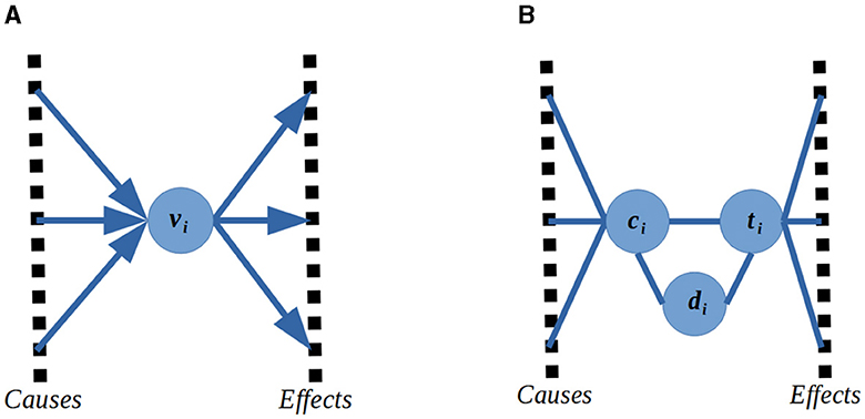
Figure 1. A cause–effect relationship that is modeled with a directed graphical model between variables v in SCM can (it is not required to) be modeled using an undirected graphical model over variables c, d, and t in ESCM. The exogenous variables are not displayed in this figure. They are inputs to functions that output the values of variables, and in that regard, they would be on the cause side (in that, inputs can be argued to cause outputs of a function). No changes in U are made in an intervention, so they do not contribute to the understanding of the relationships between the modeled causes. (A) SCM case. (B) ESCM case.
The link between variables in the ESCM and SCM is established through the functions that are used. In SCM, there is no explicit mention of a set of functions (like in ESCM) that implements a change of definition of variables in V and no set of variables (like D in ESCM) that characterizes the behavior of those functions. It is the usage of and that motivates the replacement of V in SCM by C and T in ESCM. In ESCM, the functions in and in take distinct sets of variables as inputs (a function in takes variables in the sets U and T while a function in takes variables in the sets C and D), and their output values are attributed to distinct sets of variables (the outputs of functions in are assigned to variables in C and the outputs of functions in are assigned to variables in T). An asymmetric causal relation between variables in SCM is easier to express in ESCM because: (1) the sets of variables in the inputs and outputs of both and are disjoint and (2) there is asymmetry in the information in C and T.
For two variables {ve, vc}∈V in a SCM that correspond to the sets {cc, dc, tc} and {ce, de, te} in an ESCM, we have that which expresses an asymmetric relation in the sense that it is different from cc = fc(te, ...). This contrasts with SCM where a single variable v refers to both information pertaining to the respective c and t, and for that reason, arrows in a graphical model (see Figure 1) are necessary to express the asymmetry of causal relationships. The asymmetry in models is further discussed in the Supplementary material.
A causal relation in ESCM is defined by setting which variables in T are arguments in a function that outputs the value of a variable in C and hence:
Lemma 0.0.1. A causal relation in a model implies the existence of a constraint of the type expressed in Equation 1.
Proof. Cause–effect relationships define the arguments of functions in a model, and by definition, a function only depends on its inputs. This essentially derives from the independence assumption of a variable's output from the non-causes of this variable in the SCM. ☐
Corollary 0.0.1.1. The zero sensitivity of a causal model to some variable can be assessed through cause–effect relationships using the chain rule for derivatives, without needing to specify the functions the model decomposes to.
3 Tractable probabilistic models
Current TPMs, namely, probabilistic generating circuit (PGC) (Zhang et al., 2021) ⊃ SPN (Poon and Domingos, 2011) ⊃ arithmetic circuit (AC) (Darwiche, 2002) ⊃ PSDD (Kisa et al., 2014), are defined as recursive calls of functions defined over a semiring with operations ⊕, ⊗ (Friesen and Domingos, 2016) and get their properties via structural constraints (Shen et al., 2016; Choi and Darwiche, 2017). A clear example appears in the PSDD literature. The structure of PSDD is based on Sentential Decision Diagrams (SDD) (Darwiche, 2011). SDD are defined with ⊕ and ⊗ as ∨ and ∧ over Boolean values. Despite PSDD being functions in ℝ+ where ⊕ is + and ⊗ is × , it is common in PSDD-like structures to draw analogies between the two different semirings. The least amount of structural constraints that is imposed in order to ensure the construction2 of a model with tractable marginalization contains the properties:
1. Decomposability (Friesen and Domingos, 2016), that imposes that the scope of each function under a product node is disjoint from the rest. Decomposability allows summation operations of marginalization at the output to be pushed, through the product operations using only properties of operations in a semi-ring. For two disjoint sets of variables A and B and two functions fa and fb, we have that ∫fb(B) × fa(A) =∫fa(A)×∫fb(B). Decomposability allows an integration operation, at the output node of the CG of the TPM, to be implemented at the input nodes of the CG of the TPM.
2. Smoothness (Friesen and Domingos, 2016), that imposes that the scope of each function under a summation node is the same. In a smooth and decomposable model, marginalization of variables can be done with integration at either the output or input nodes of the CG of the TPM (Choi and Darwiche, 2017). This relation between integration and marginalization is not guaranteed in models that are decomposable and not smooth (Choi and Darwiche, 2017).
It will be assumed that all computations are performed explicitly, that is, there are no edge weights in the CG. This does not affect the size more than a constant factor as every such input could be replaced by one multiplication. The structural properties of current TPM depend on scope partitions; hence, the question of how to handle scope arising from the parameters is pertinent. When the parameters are not outputs of functions, it is considered that they do not contribute to the scope which enables us to rule out smoothness and decomposability related issues arising from parameters in that case. When the parameters are functions of some variables in the model, they contribute to the scope of the overall model. In that case instead of thinking of the TPM as a model over the initial variables, we should think of it as a model over the augmented set of variables that includes the parameter variables.
3.1 Orders and causality in TPM
As a consequence of imposing smoothness and decomposability to a CG3 of a TPM and by construction in the case of PGC (Zhang et al., 2021), we get that all variables that appear at the input layer and the internal nodes of the CG are functions of increasing scope; thus, we do not have explicit statements that any variable is defined as a function of any other variable. In ESCM, the cause–effect relationships are defined over derived variables; hence, they imply the existence of a decomposition over functions whereby a cause–effect relationship means the cause is an argument to the effect function. In TPM, we can represent a decomposition over functions of increasing scope, e.g., . When a variable enters the CG alongside or after its causes, a function decomposition that does not contradict the cause–effect constraints is encoded in the CG. In order to apply the notion of functions that replace information of the modeled causes by information pertaining to an intervention (see Section 2) in a smooth and decomposable TPM, the following strategy, illustrated in Figure 2, can be used:
1. Combine information pertaining to a variable, its modeled causes, and the exogenous variables it depends on. In the example from Figure 2, this corresponds to ;
2. Combine the information obtained as output from the last step with information pertaining indicator functions for the different interventional cases. In Figure 2, those indicator functions are represented by: (a)  that stands for an intervention that sets the value of de to true, (b)
  that stands for an intervention that sets the value of de to false, and (c)
  that stands for the absence of interventions . This step is similar to the previous one in that we use the ⊗ operation so that we can reference each of the combinations of the states Val(tc, ce, de) individually.
3. Combine each of the ith Val(tc, ce, de) with a parameter (θi) so that we can: (a) attribute to each of the states a different likelihood of occurrence and (b) guarantee, via local normalization (Peharz et al., 2015), that we can make the output of each ⊕ node to sum up to 1⊗ when the function they compute is marginalized . These parameters refer to the likelihoods of the values of endogenous variables and states of D, so they refer to ;
4. Combine the information obtained as output from the last step with indicator functions for the states of te;
5. Merge the information spread across multiple nodes with the ⊕ operation, e.g., in Figure 2 we have that where i stands for the index that identifies the parameter corresponding to the state representation {te, tc, pstate};
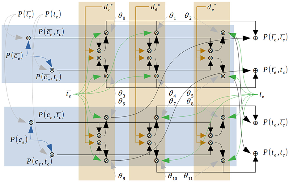
Figure 2. Illustrative example for the computation of the joint probabilities of full information pertaining to a variable and its modeled causes . This example corresponds to the situation in Asia dataset (see Section 4). No exogenous variables are declared for that dataset, it is assumed that they are not referenced, and thus, they are considered to be marginalized. The information pertaining to the multiple sources of information is combined using ⊗ operation, and we get a layer where we can reference any Val(tc, ce, de, te). Then, the information regarding Val(tc, te) that is spread across multiple ⊗ nodes is aggregated in ⊕ nodes.
The second step only increases the size of a CG that does not reference D directly (uses an external algorithm to modify the model in case of interventions) by a factor that depends linearly on the number of states of a variable. This procedure can be implemented one time per variable independently. Therefore, choosing to represent explicitly the algorithm that changes the variable definitions when the information pertaining to effects is not processed before information pertaining to causes yields in the worst case a CG that is bigger by a factor of the number of variables and the maximum number of states of a variable in the model. The procedure present in Figure 2 replaces the information pertaining to some c by information pertaining to the corresponding t, provided that we can choose a value for the indicator functions that depend on d such that:
1. The output of ⊗ is equal to the other input of the operation. In order for the value to attribute to d be independent of the other value in the computation that goes on, there should exist a neutral element of ⊗ (1⊗)4 and an indicator function that depends on d should be able to take that value. This ensures that according to the value of d, the other term in ⊗ can pass unchanged.
2. The output of ⊗ is the neutral element of ⊕ (0⊕)5. In order for the value to attribute to d be independent of the computation that goes on, there should exist an absorbing element of ⊗ (0⊗)6 such that the output of ⊗ can be made to solely depend on the indicator function over d and that value should be equal to the neutral element of ⊕, i.e., 0⊗ = 0⊕. This ensures that according to the value of d, some term in ⊕ can be “cut off”.
Although the value of t can be indexed with a combination of c and d, in Figure 2, it can be seen that choosing the nodes referring to value(s) of de (brown boxes) and referring to value(s) of ce (blue boxes), multiple queries are necessary to reference the nodes corresponding to value(s) of te. Due to the scope constraints of TPM it can be stated that the set of smooth and decomposable structures allowable for a TPM with U, D, C, and T labels is not greater than those that use only U and D. Keeping in mind that tractable marginalization in TPM is only assured for labeled variables with indicator functions, a decision for including an indicator function for any derived variable should be weighted with our intent to use it.
3.2 Causality through constraints and TPM
When modeling causality as constraints over a space of functions, it is paramount to define those constraints. They are not required to come from a priori knowledge and, just as the rest of the parameters of a model, can be learned from data. In this case, a constraint is given indirectly through the objective function and the data. Executing all computations of a TPM in parallel requires exponential size as, to aggregate the probabilities over a single ⊕ node, all combinations of values of variables should be referenced. This means that in order to get a more compact model, some order should be imposed over the computations in the CG. This raises the question of how to choose such an order. Toward that end, cause–effect relationships can offer a notion of locality as the set of cause–effect relationships among variables defines the Markov Blanket of a cluster {c, d, t} of variables. Beyond that, cause–effect relationships provide a function decomposition and an implicit order for the execution of computations. The methodology expressed in Section 3.1 is one example of a process for describing a TPM where the cause–effect orders are used in the sense that no effect appears in the scope of a function before its causes. Performing the computations in an order other than that implied by a cause–effect relationship does not prevent a model from computing the correct outputs. Consider that the cause–effect relationship should hold for the model. A CG may have a function decomposition consistent with in which case information pertaining to fc() should be stored until it is used in the estimation of fe() given its modeled causes. A CG may also have a function decomposition consistent with , then fe(), all its modeled causes and all its modeled effects should be stored (see Figure 3) until we get to estimate fc(), after which all computations regarding fe() that were postponed can be computed exactly, based on ground truth definitions, followed by the computations of the effects of fe() whose estimation was also postponed. It should be noted that the necessity to store the values corresponds to the worst case where the information of the modeled causes is required to accurately perform the estimation of its effects and no information about either the modeled causes or the effects can be reliably estimated using other sources of information available to the model. In that scenario, it can be stated that choosing not to use an order of computations compatible with the causal order leads to either a non-optimal space requirement or performance loss.
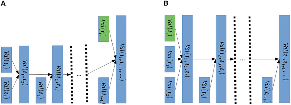
Figure 3. Example of “storage” of information about a variable in a CG of a TPM. Each of the blocks represents a layer of operations in a CG, and the dotted lines are used to reference an arbitrary continuation of the CG. While both Figures refer to the same input–output behavior, they are implemented with a different CG. The green color is used to highlight the block of information that is introduced earlier in the CG of the right Figure. The relative sizes of the rectangles represent the size of Val(...). (A) Without “storage”. (B) With “storage”.
Due to the distributive properties of a semiring, we have that ∀xa, b, c:xa⊗(xb⊕xc) = (xa⊗xb)⊕(xa⊗xc). This means that the ⊗ operations can be pushed down the CG. Applying the distributive property to push down a layer of ⊗ operations increases the scope of that layer. This is problematic in decomposable and smooth TPM (like SPN) as these properties imply that: (a) the ⊕ operation only merges information with the same scope; (b) different variables ought to be combined with a ⊗ layer, and (c) the function described by the model is multilinear, i.e., it is a summation and each term is a product of states of variables, e.g., . Therefore, introducing a variable earlier in a smooth and decomposable CG prevents us from introducing it again later, with an ⊗ operation, in a computation that already depends on it. Moreover, as the ⊕ operation is used to aggregate information about the multiple states of the variables (e.g., captures information about both states of x2), computations that depend on some ⊕ operation are not able to discriminate between the states they take as input (individually) that hinders our ability to “sum out” (to decrease the number of nodes we can index7 in a layer) from the CG information that is introduced too early and that we only intend to use later.
4 Experiments
4.1 Experimental goals
The goal of the experiments is to empirically demonstrate/disprove the assertion made in Section 3.2 that not using a cause–effect order in smooth and decomposable TPM can lead to a bigger model for some level of performance. It is considered that an example of occurrence of the phenomenon theorized in Section 3.2 is sufficient to show that it exists. The goal of this section is not to ascertain how likely it is to occur or through empirical means discuss in depth the cases in which it does occur. The models ought to be compared with the metric expressed in Equation 2 where Modeli stands for an arbitrary model, dpnt to a data point and interventions∈dpnt to the intervention expressed in the data point. It expresses the average logarithm of the likelihood of observing each data point given that the specific intervention of that data point occurred in the test dataset given a model (with parameters learned from the train dataset). A model compatible with the correct cause–effect structure is to be compared to a series of models with increasing parameters and a wrong “cause–effect” structure.
4.2 Experimental methodology
4.2.1 Data
Three datasets are used in the experiments:(1) Asia dataset (Lauritzen and Spiegelhalter, 1988), (2) a synthetic dataset created to illustrate the point of this study, and (3) Earthquake dataset (Korb and Nicholson, 2010) . Two of these datasets are used in the experiments conducted and presented in the main study, while the results using the third dataset are presented in Supplementary material.
All variables in the Asia dataset (Lauritzen and Spiegelhalter, 1988) v0) “smoke”, v1) “bronc”, v2) “lung”, v3) “asia”,v4) “tub”,v5) “either”,v6) “dysp” and v7) “xray” are binary. To the ground truth distribution interventions over the variables (a) “lung” (d2), (b) “tub” (d4), (c) “either” (d5) and (d) “dysp” (d6) were added according to the cause–effect relationships expressed in Figure 4A where arrows point from causes to effects. Each of the variables in the set D has three possible values, one corresponding to the absence of intervention over the corresponding endogenous variable and two corresponding to setting the value of the intervened variable to either of the values it can take. Existence and type of interventions were determined independently for each variable in D2, 4, 5, 6. To the absence of intervention for each variable was assigned probability 50%. The likelihood over the rest of the states8 of the variables D2, 4, 5, 6 was determined so that interventions replaced the probability distribution over the states of the corresponding variable that depended on the modeled causes by a value9 sampled from a uniform distribution. The synthetic dataset was created according to the cause–effect relationships expressed in Figure 5A where arrows point from causes to effects. The conditional likelihoods related to the CBN used for generating the samples are provided in the Supplementary material. Of the seven binary variables V0, 1, 2, 3, 4, 5, 6, only V1, V3, and V5 were intervened. For each of the intervened variables, the likelihood of no intervention was 50%. The likelihood over the rest of the states8 was determined so that interventions replaced the probability distribution over the states of the corresponding variable that depended on the modeled causes by a value9 sampled from a uniform distribution.
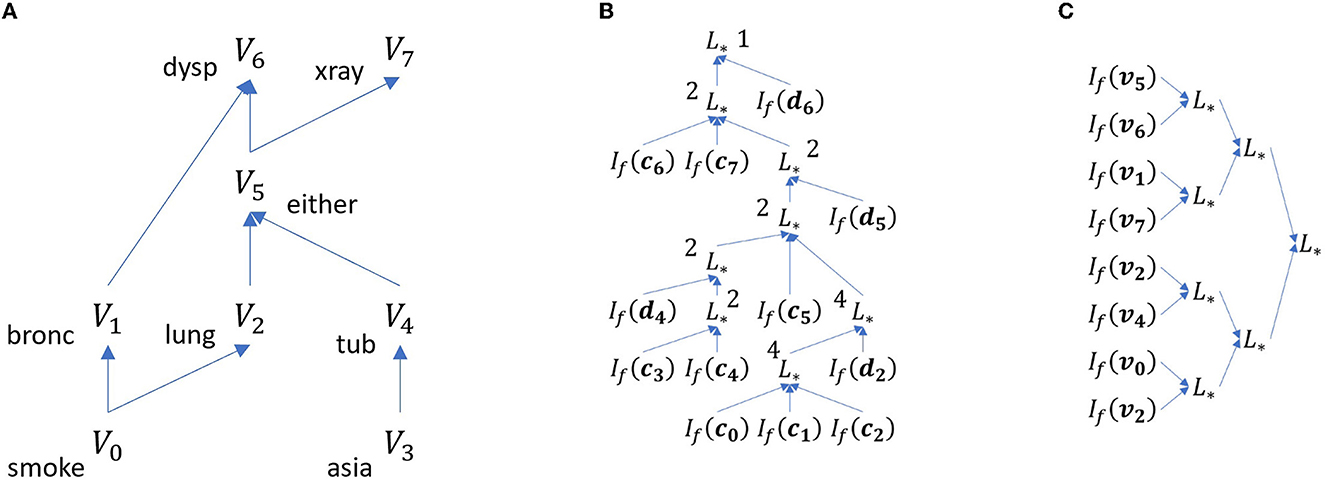
Figure 4. Decompositions of functions according to the ground truth (A) and Equations (3) (B) and (4) (C). (A) Cause–Effect Relationships in Asia dataset (Lauritzen and Spiegelhalter, 1988). Arrows point from causes to effects. (B) Structure of a model given by Equation 3. The numbers next to L* represent the number of ⊕ nodes the layer has. (C) Structure of a model given by Equation (4).
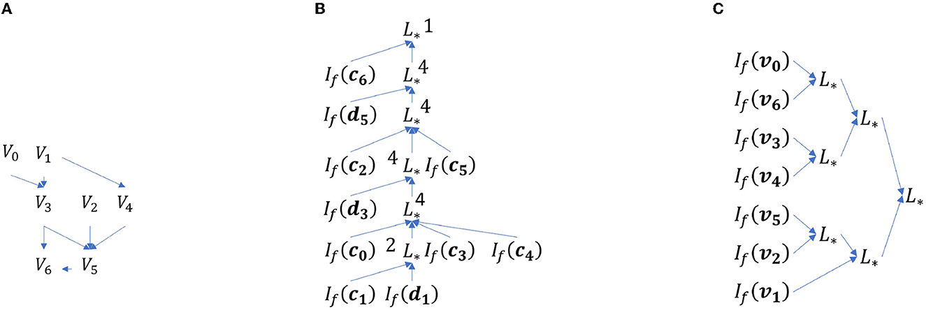
Figure 5. Decompositions of functions according to the ground truth (A), and Equations (5) (B) and (6) (C). (A) Cause-effect relationships in a synthetic dataset. Arrows point from causes to effects. (B) Structure of a model given by Equation 5. The numbers next to L* represent the number of ⊕ nodes the layer has. (C) Structure of a model given by Equation (6).
For both datasets, 50,000 samples were created, and a random split was used for separating the training data (80%) from the test data (20%).
4.2.2 Models
Two types of models using the semiring of summation (+) and multiplication ( × ) over the non-negative real numbers were used in the experiments. In the first type (TypeOrd), we used structures consistent with the cause–effect relationships in the respective datasets and can be considered a compilation from the ground truth ESCM using variable elimination. For the Asia dataset, the TypeOrd model is expressed in Equation (3) and Figure 4B and for the synthetic dataset is expressed in Equation (5) and Figure 5B. For the second type of model (TypeTree), the structure expressed in Equation (4) and Figure 4C and Equation (6) and Figure 5C was used for the Asia and synthetic dataset, respectively. The structure of TypeTree does not adhere to the cause–effect relationships in the sense that, according to Section 3.2, for exact output computation under the worst of cases, some of the structure should act as storage. The second type of structure, similarly to iSPN, is a tree where at each layer of ⊗ operations, each input has half of the variables and the parameters are the outputs of a neural network. The neural network has three intermediate layers with a constant width of 20, and the non-linearity used was the LeakyReLU with negative slope of 0.01. All layers use a bias term. The weights were initialized with the kaiming_uniform_ (He et al., 2015) implementation from pytorch. It should be noted that the second type of model, contrary to iSPN (Zečević et al., 2021), uses discrete indicator functions for the leaf distributions.
The T labels were omitted in the first type of model as they were not used to index the data in training or evaluation. In the second type of model, no cause–effect consistent order is used in the function decomposition and information pertaining any intervention can enter everywhere there is a parameter. The joint probabilities over subsets of variables we read at any point along the respective CG do not necessarily correspond to the partition we get according to an ESCM under which we can state that in some node we can read the joint probability of some variable and its modeled causes.
Three instances of the second type of model (see Equations 4, 6 and Figures 4C, 5C) were used in the experiments for each dataset. They have 2n nodes in the ⊕ layers, with n = 1, n = 2, and n = 4, yielding models with 52, 208, and 1,216 parameters that are outputs of neural networks for the Asia dataset; hence, they are called Tree52, Tree208, and Tree1216. For the synthetic dataset the number of parameters is 44, 160, and 800; hence, they are called Tree44, Tree160, and Tree800.
The implementation of Equation (3) (see Figure 4B) has a total of 288 parameters of which only 86 are non-zero, so it was called Ord86. For the synthetic dataset, the implementation of TypeOrd (see Equation 5 and Figure 5B) the total number of parameters is 212 of which only 70 are non-zero, so it was called Ord70.
4.3 Training
The TypeOrd models were trained with the model counting approach (Kisa et al., 2014; Peharz et al., 2014) that is guaranteed to provide the maximum likelihood parameters(which corresponds to a lower loss according to Equation 7). The structure used by TypeOrd corresponds to the model that generates the data. The data generation procedure from a SPN (Poon and Domingos, 2011) amounts to choosing at each ⊕ node a branch with likelihood equal to the respective weight divided by the sum of all weights of all the inputs of the ⊕ node. Therefore, it can be stated that data generated by each of the learned TypeOrd are indistinguishable from the data generated by the ground truth model. In this context, the CBN network used to generate the data for the experiments can be interpreted as a way of assigning parameters to each of the TypeOrd that could have been used to generate it. Multiple distinct models with the correct input–output characteristics can exist, and in Section 3.2, it is argued that a structure that does not adhere to the cause–effect relationships can correctly model the input–output relationships by increasing its size. The comparison between TypeOrd models built using the cause–effect relations of the CBN and each of the TypeTree models that do not rely on them empirically evaluates the impact of structure in the performance of models. RatioOfCountsTr corresponds to counting the events that occurred without assuming any structure [e.g., Using some structure according to which P(event1, event2) = P(event1) × P(event2), the act of counting joint occurrences of event1 and event2 is replaced by counting their occurrences separately and multiplying the results]. Both types of models (iSPN-like and TypeOrd) contain function compositions since they are not implemented as a single (L*) layer model where each joint occurrence of events has a distinct parameter (see Equations 3–6). In the worst of cases, the argument for correctness of models without a structure that captures properties of the data generation algorithm calls for storing all information in the layers leading to one weight per occurrence of each type of joint events (Section 3.1) which is embodied in RatioOfCountsTr.
The TypeTree models do not have the structural properties that ensure the correctness of the training procedure used for the TypeOrd models; therefore, a training method that does not have guarantees of reaching an optimal set of parameters was used. They were trained 10 times for 10 epochs with the Adam optimizer (Maclaurin et al., 2015) with the default parameters, batch of 100 with the objective to minimize10 the loss function defined in Equation (7) where |batch| stands for batch size, and dpnt stands for a sample. A sample has information pertaining to C and D. The parameters of the iSPN-like model are dependent on the interventions, so a single query for the SPN part of model for P(dpnt) using parameters given by feeding to the neural network the respective intervention yields P(dpnt|interventions∈dpnt).
4.4 Experimental results
The results are shown in Figures 6–13, where the height of each bar stands for the mean of a value over the repetitions of the experiments and the error bar has the height of two standard deviations over the repetitions of the experiments. In Figure 6, the absolute value of the average of the logarithm of the likelihood of observing the data in the test dataset given that the intervention took place is plotted. This value is minimized during training (for the training dataset that is drawn from the same statistical distribution as the test dataset), and a lower value corresponds to better modeling the data. Figures 7–11 present results obtained using the Asia dataset, while Figures 12, 13 present results using the synthetic dataset. In Figures 7, 8, there are examples of answers to conditional likelihood queries for different models. In Figures 9, 10, the queries contain multiple interventions. The queries P(c6 |  ,
,  ,
,  ,
,  )and P(c7 |
  ,
,  ,
,  ,
,  ) in Figures 9, 10 correspond to a soft intervention scenario not observed during training. For these queries, the height of RatioOfCountsTr is the average of the likelihoods over four separate interventional cases due to the multi-linearity of the table-like model that sums over each set of joint events. In Figure 11, the likelihood of queries pertaining to variables in the set T is presented for the Ord86 model only as they pertain to information about both variables in C and variables in D and cannot be formed only from conditional likelihoods available in the second type of model. In Figure 12A, an example of different query responses for the different models used for the synthetic dataset is presented. Figures 12B, C show queries that highlight the differences between interventions in a cause or non-cause of a variable in its c value are presented. In Figure 13, the queries pertain to multiple interventions.
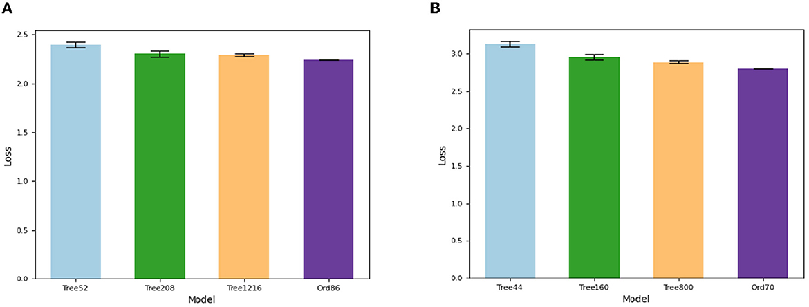
Figure 6. Absolute value of the average of logarithm of conditional likelihood of observing the test data given that the respective intervention took place (see Equation 2). That value corresponds to the loss over the test dataset in the case in which the batch size is equal to the size of the test dataset (Equation 7). Lower is better. (A) Asia dataset. (B) Synthetic dataset.
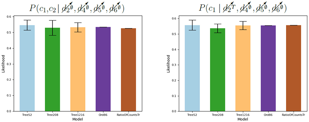
Figure 7. Examples of conditional query responses corresponding to two cases where t2 is true.
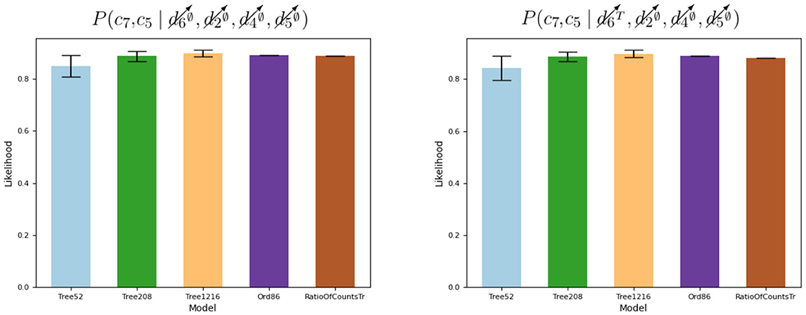
Figure 8. Effect of knowledge about v6 in v7 given v5.
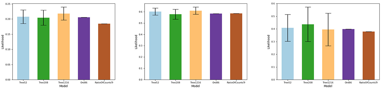
Figure 9. Conditional likelihood for the queries P(c6 |  , P(c6 |
  , and P(c6 |
  .
.
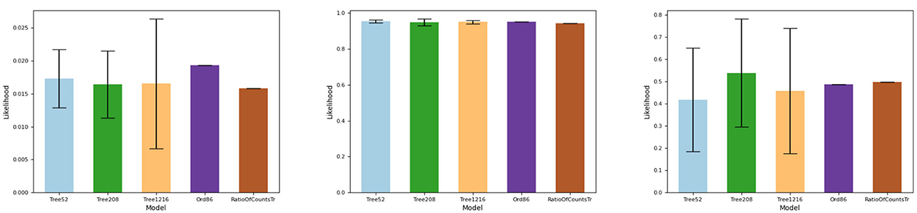
Figure 10. Conditional likelihood for the queries P(c7 |  , P(c7 |
  , and P(c7 |
  .
.
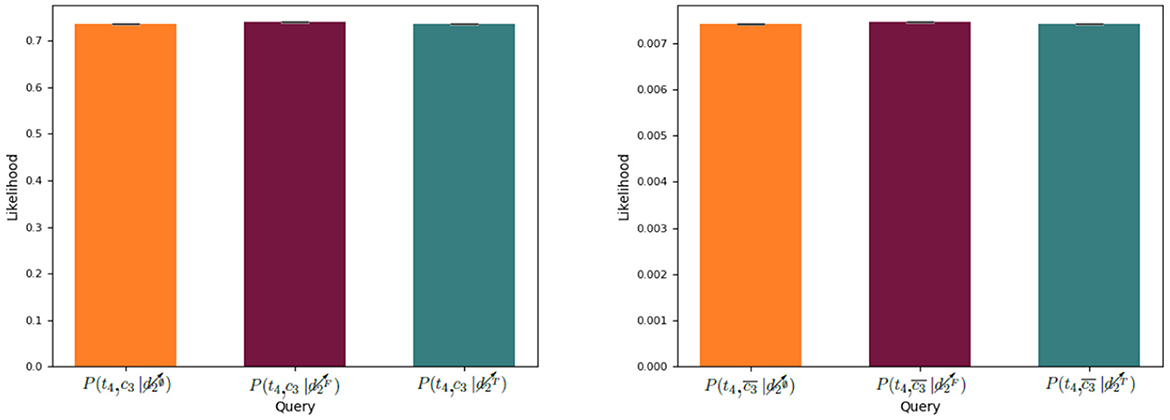
Figure 11. Impact in c3 and t4 of knowledge about d2. For Ord86, P(t4, c3, d2) = P(t4, c3)P(d2) so P(t4, c3|d2) = P(t4, c3).
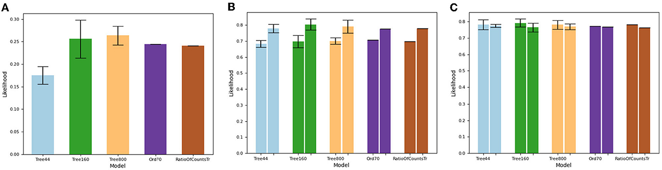
Figure 12. Differences in responses to queries and impact of interventions in causes and non-causes of a variable. (A) Response to query P(c5, | . (B) Impact of interventions in causes of a variable. The left and right bars for each mode correspond to the queries, P(c6 |
  and P(c6 |
  , respectively. (C) Impact of interventions in non-causes of a variable. The left and right bars for each mode correspond to the queries, P(c3 |
  and P(c3 |
  , respectively.
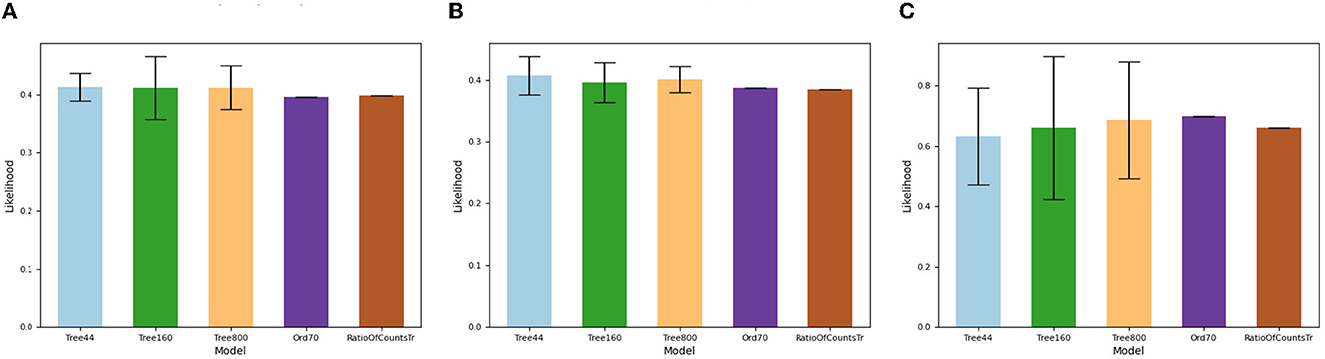
Figure 13. Extrapolation from queries not observed during training. (A) Response to query P(c6 |  . (B) Response to query P(c6 |
  . (C) Response to query P(c6 |
  .
.
5 Discussion
In Figure 6, it can be seen that the best results were obtained with the first type of model (TypeOrd) and that the more parameters in the second type of model, the better the results. This empirically validates the argument in Section 3.2 that for smooth and decomposable TPM, not adhering to an order of computations expected from the function decomposition implied by a set of cause–effect relationships can increase the amount of parameters required to yield some level of accuracy. This is also corroborated (for the case of the Asia dataset) by the number of parameters used in iSPN (Zečević et al., 2021) that for each interventional case and the same dataset ranged from 600 to 3,200 in increments of 600, which is much bigger than 86 used in Ord86 for all interventional cases. The first type of model can be seen in light of the second type as a model where: (a) each of the parameters is a function of a constant bias term, (b) there exist indicator functions for both the observations and interventions of variables, and (c) the structure of the CG is constructed based on cause–effect relationships so that information about effects is not processed before information about their causes . While the second type of model behaves as an SPN for each intervention case, the first type of model is a TPM over observations and interventions.
A set of cause–effect relationships implies the existence of a function decomposition (see Section 2) that reduces the number of parameters for a model but yields no information about the values of the non-zero parameters. This makes the space of functions considered for the first type of model used in the experiments much smaller than that of the second type of model that does not use a principled way of trimming down the number of hypothetically good models before looking at the training data. There is a parallel between the construction of the TPM based on processing information pertaining to causes before the effects in a CG and the variable elimination algorithm used in Darwiche (2022). In both, we have that: (a) information about a cluster of variables is created with a layer of ⊗ operations, and (b) a set of conditional independence relations that follow from the cause–effect relationships allows us to state that the value of some variable that is yet to be included in the CG does not depend on some variable already in the CG which in turn allows us to aggregate information with ⊕ nodes. In the second type of model, the clusters we make do not rely on the cause–effect relationships to choose an order by which information is processed. Therefore, we cannot necessarily use the conditional independence relations to rule out at each ⊗ layer some of the information. The size of a cluster of variables increases exponentially with the number of variables; hence, in the worst of cases, for an exact answer, the number of states we can have in one layer of the model can become exponentially bigger. It is known that the order of variable elimination can lead to expressions of different sizes for the same input–output behavior (Koller and Friedman, 2009). However, the structure of the second type of model is not amenable to such an analogy as the clusters we express in the CG do not capture all the neighbors of a variable in a ground truth undirected graphical model, which would lead to over-sized clusters before each “elimination” of a variable. Moreover, it can be stated that the lack of constraints over the space of functions prevents the extrapolation of results to cases that are either absent or are rare in the dataset.
In Figure 12A, it can be verified that the different models fitted to the synthetic dataset give different answers to queries. In Figure 12B, it can be seen that an intervention on a cause of a variable can impact its c value. In Figure 12C, it can be observed by comparison of the bars RatioOfCountsTr that an intervention on a non-cause of a variable has nearly the same number of samples but not exactly the same. This is attributed to random sampling generation and finite dataset size. The TypeOrd model is closer to the RatioOfCountsTr than TypeTree models that also vary more between the two queries.
As an artifact of random sampling on data generation and finite dataset size, there is a difference (see Figures 7–10) in the height of the bars for Ord86 that corresponds to model counting with a factorization compatible with the data generation and the bars for RatioOfCountsTr that corresponds to model counting without a factorization. In Figures 7, 8, the mean responses to queries over the second type of model are within one standard deviation from Ord86, but they are far from both Ord86 and RatioOfCountsTr in the rightmost graphs shown in Figures 9, 10 that correspond to scenarios with two interventions that set the intervened variables to a uniform distribution. In TypeOrd models, the structure allows the extrapolation to be performed correctly but the same cannot be said for the neural network that provided the parameters for each of the iSPN-like models. The same issue can be observed in Figure 13. The neural networks used for the TypeTree models have only been trained on inputs with values one or zero which left the function that ought to be learned undefined in between, that is, no constraints (other than the function being piece-wise linear due to the activation functions of the neurons) were imposed on how the outputs of the neural networks should change as inputs vary from zero to one. More than a problem of lack of structure in the SPN to which the parameters are assigned, this is a problem of generalization(extrapolation to cases not observed during training) as the height of the bar RatioOfCountsTr is close to TypeOrd.
Another significant difference is that for iSPN-like models, where interventions are used only for providing the weights of an SPN, we cannot compute joint likelihoods involving different interventional cases. An example of such queries is present in Figure 11 where  . The joint likelihoods of t4 and c3 are computed with L*(L*(If(c3), If(c4)), If(d4)) which is a different branch from where d2 is computed (see Figure 4B). Therefore, the value of each joint likelihood query over Val(c3, t4) conditioned on the intervention over d2 does not depend on d2 as P(c3, t4, d2) = P(c3, t4)P(d2) which implies that .
6 Conclusion
Causal assertions stem from an asymmetric relation between some variable, its causes, and effects. Both the causes and effects are correlated with information about the state of a variable. A variable is only correlated with the partial information about its effects which does not include factors of variation outside of the modeled ones (e.g., Interventions). However, by definition, a variable is correlated with the full information pertaining its causes, something that is not accessible without simplifying assumptions. By making those assumptions explicit, structural causal models are extended and causality is defined as a constraint over the function space of a higher dimensional model. Current TPM and cause–effect relationships imply distinct function decompositions. In the decomposition implied by cause–effect relationships, the endogenous variables are outputs of functions and in the TPM they are inputs in the model. The mismatch is only apparent because it is resolved when taking an input–output perspective as in both cases exogenous variables exist and all aspects of both models depend on them. The process of answering queries pertaining to interventions with SCM uses an algorithm external to the SCM to adapt its structure for the execution of that intervention. This is not the case with ESCM where that process is included in the model through the set of functions . Therefore, by using ESCM instead of SCM as a starting point for compilation of TPM, the usage of an algorithm external to the model that changes it in order to adapt it to answer questions pertaining to interventions was avoided. It was shown that implementing that algorithm explicitly leads to a TPM that in the worst case has a linear size increase in the number of variables and the maximum number of states of a variable. Sufficient conditions for implementing it in a generalization of current classes of TPM to other semirings are stated. The functional approach is used to unify under one framework the distinct approaches for modeling TPM with causality. It enables us to both explain adherence to cause–effect constraints without explicit structure in a function decomposition as in iSPN (Zečević et al., 2021) and the role of structure in compilations from SCM to TPM (Darwiche, 2022) as an implicit way of imposing constraints over a function space. It was discussed and shown empirically that choosing not to adhere to a function decomposition consistent with an order implied by a set of cause–effect relationships can lead to a big increase in size requirements for a smooth and decomposable TPM.
Data availability statement
The raw data supporting the conclusions of this article will be made available by the authors, without undue reservation.
Author contributions
DC: Conceptualization, Formal analysis, Investigation, Methodology, Resources, Software, Visualization, Writing—original draft. JB: Formal Analysis, Supervision, Validation, Writing—review & editing.
Funding
The author(s) declare financial support was received for the research, authorship, and/or publication of this article. This research was supported by the Portuguese Foundation for Science and Technology (FCT) under grant 2020.09139.BD. This study was also supported by the Portuguese Foundation for Science and Technology (FCT) under the project UIDP/00048/2020.
Conflict of interest
The authors declare that the research was conducted in the absence of any commercial or financial relationships that could be construed as a potential conflict of interest.
Publisher's note
All claims expressed in this article are solely those of the authors and do not necessarily represent those of their affiliated organizations, or those of the publisher, the editors and the reviewers. Any product that may be evaluated in this article, or claim that may be made by its manufacturer, is not guaranteed or endorsed by the publisher.
Supplementary material
The Supplementary Material for this article can be found online at: https://www.frontiersin.org/articles/10.3389/fcomp.2023.1263386/full#supplementary-material
Footnotes
1. ^Assuming P≠NP≠P#P.
2. ^Although not strictly required to get a model with tractable marginalization they are commonplace appearing in construction processes from PGC (Zhang et al., 2021) to PSDD (Kisa et al., 2014).
3. ^A directed graph (N, E) where nodes (N) correspond to operations to be performed and edges (E) pointing from a node ni to a node nj indicate that the output of ni is an input of the operation nj. Nodes without edges pointing toward them are input nodes, and the operation they perform is data acquisition.
4. ^a = 1⊗⊗a = a⊗1⊗.
5. ^a = 0⊕⊕a = a⊕0⊕.
6. ^0⊗ = 0⊗⊗a = a⊗0⊗.
7. ^The combinations of indexes that can be used in a layer in the CG of a smooth and decomposable TPM determine the size of that layer. The more ways the information can be indexed the bigger the layer.
8. ^Corresponding to one of the possible interventions over the variable.
9. ^Hard interventions that set a variable to one of its possible values were used. No soft interventions that set a variable to a distribution of its values were used.
10. ^The lower the value of the loss the higher the likelihood of the data observed in the test dataset being generated by a model.
References
Bareinboim, E., Correa, J. D., Ibeling, D., and Icard, T. (2022). “On pearl's hierarchy and the foundations of causal inference,” in Probabilistic and Causal Inference: The Works of Judea Pearl, eds H. A. Geffner, R. Dechter, and J. Y. Halpern (New York, NY: Association for Computing Machinery), 507–556. Available online at: https://causalai.net/r60.pdf
Bareinboim, E., and Pearl, J. (2013). “Meta-transportability of causal effects: a formal approach,” in Artificial Intelligence and Statistics, eds C. M. Carvalho and P. Ravikumar (Scottsdale, AZ: PMLR), 135–143.
Chavira, M., and Darwiche, A. (2005). “Compiling bayesian networks with local structure,” in IJCAI, Vol. 5 (San Francisco, CA: Morgan Kaufmann Publishers Inc.), 1306–1312.
Choi, A., and Darwiche, A. (2017). “On relaxing determinism in arithmetic circuits,” in Proceedings of the 34th International Conference on Machine Learning-Vol. 70 (JMLR), 825–833.
Darwiche, A. (2002). “A logical approach to factoring belief networks,” in KR, Vol. 2 (San Francisco, CA: Morgan Kaufmann Publishers Inc.), 409–420.
Darwiche, A. (2011). “Sdd: A new canonical representation of propositional knowledge bases,” in Twenty-Second International Joint Conference on Artificial Intelligence (AAAI Press).
Darwiche, A. (2022). Causal inference using tractable circuits. arXiv. doi: 10.48550/arXiv.2202.02891
Erikssont, J., Gulliksson, M., Lindström, P., and Wedin, P.-A. A. (1998). Regularization tools for training large feed-forward neural networks using automatic differentiation. Optimiz. Methods Softw. 10, 49–69. doi: 10.1080/10556789808805701
Friesen, A., and Domingos, P. (2016). “The sum-product theorem: A foundation for learning tractable models,” in Proceedings of The 33rd International Conference on Machine Learning, volume 48 of Proceedings of Machine Learning Research, eds M. F. Balcan, and K. Q. Weinberger (New York, NY: PMLR), 1909–1918.
He, K., Zhang, X., Ren, S., and Sun, J. (2015). “Delving deep into rectifiers: Surpassing human-level performance on imagenet classification,” in Proceedings of the IEEE International Conference on Computer Vision (IEEE Computer Society), 1026–1034.
Jalaldoust, K., and Bareinboim, E. (2023). Transportable Representations for Out-of-Distribution Generalization. Technical Report R-99, Causal Artificial Intelligence Lab, Columbia University.
Kisa, D., Van den Broeck, G., Choi, A., and Darwiche, A. (2014). “Probabilistic sentential decision diagrams,” in Fourteenth International Conference on the Principles of Knowledge Representation and Reasoning (AAAI Press).
Koller, D., and Friedman, N. (2009). Probabilistic Graphical Models: Principles and Techniques. The MIT Press.
Lauritzen, S. L., and Spiegelhalter, D. J. (1988). Local computations with probabilities on graphical structures and their application to expert systems. J. R. Stat. Soc. 50, 157–194. doi: 10.1111/j.2517-6161.1988.tb01721.x
Maclaurin, D., Duvenaud, D., and Adams, R. (2015). “Gradient-based hyperparameter optimization through reversible learning,” in International Conference on Machine Learning (JMLR), 2113–2122.
Mohan, K., and Pearl, J. (2021). Graphical models for processing missing data. J. Am. Stat. Assoc. 116, 1023–1037. doi: 10.1080/01621459.2021.1874961
Papantonis, I., and Belle, V. (2020). Interventions and counterfactuals in tractable probabilistic models: Limitations of contemporary transformations. arXiv. doi: 10.48550/arXiv.2001.10905
Pearl, J. (2019). The seven tools of causal inference, with reflections on machine learning. Commun. ACM 62, 54–60. doi: 10.1145/3241036
Pearl, J., and Bareinboim, E. (2014). External validity: from do-calculus to transportability across populations. Stat. Sci. 29, 579–595. doi: 10.1214/14-STS486
Peharz, R., Gens, R., and Domingos, P. (2014). “Learning selective sum-product networks,” in 31st International Conference on Machine Learning (ICML2014) (Beijing).
Peharz, R., Lang, S., Vergari, A., Stelzner, K., Molina, A., Trapp, M., et al. (2020). “Einsum networks: fast and scalable learning of tractable probabilistic circuits,” in International Conference on Machine Learning (PMLR), 7563–7574.
Peharz, R., Tschiatschek, S., Pernkopf, F., and Domingos, P. (2015). “On theoretical properties of sum-product networks,” in Artificial Intelligence and Statistics (San Diego, CA: PMLR), 744–752.
Poon, H., and Domingos, P. (2011). “Sum-product networks: a new deep architecture,” in 2011 IEEE International Conference on Computer Vision Workshops (ICCV Workshops) (IEEE), 689–690.
Shen, Y., Choi, A., and Darwiche, A. (2016). “Tractable operations for arithmetic circuits of probabilistic models,” in Advances in Neural Information Processing Systems, D. D. Lee and U. von Luxburg (Red Hook, NY: Curran Associates Inc.), 3936–3944. Available online at: https://papers.nips.cc/paper_files/paper/2016/hash/5a7f963e5e0504740c3a6b10bb6d4fa5-Abstract.html
Tikka, S., Hyttinen, A., and Karvanen, J. (2019). Identifying causal effects via context-specific independence relations. Adv. Neural Inf. Process. Syst. 32. Available online at: https://proceedings.neurips.cc/paper/2019/hash/d88518acbcc3d08d1f18da62f9bb26ec-Abstract.html
Trapp, M., Peharz, R., Ge, H., Pernkopf, F., and Ghahramani, Z. (2019). Bayesian learning of sum-product networks. Adv. Neural Inf. Process. Syst. 32. Available online at: https://arxiv.org/abs/1905.10884
Xia, K., Lee, K.-Z., Bengio, Y., and Bareinboim, E. (2021). “The causal-neural connection: expressiveness, learnability, and inference,” in Advances in Neural Information Processing Systems, Vol. 34, 10823–10836. Available online at: https://proceedings.neurips.cc/paper_files/paper/2021/file/5989add1703e4b0480f75e2390739f34-Paper.pdf
Zečcević, M., Dhami, D., Karanam, A., Natarajan, S., and Kersting, K. (2021). “Interventional sum-product networks: causal inference with tractable probabilistic models,” in Advances in Neural Information Processing Systems, Vol. 34 (Curran Associates, Inc.), 15019–15031.
Zhang, H., Juba, B., and Van den Broeck, G. (2021). “Probabilistic generating circuits,” in International Conference on Machine Learning (San Diego, CA: PMLR), 12447–12457.
Keywords: causality, tractable probabilistic models, structural causal models, function decompositions, probabilistic models
Citation: Cruz D and Batista J (2024) Causality and tractable probabilistic models. Front. Comput. Sci. 5:1263386. doi: 10.3389/fcomp.2023.1263386
Received: 19 July 2023; Accepted: 28 November 2023;
Published: 08 January 2024.
Edited by:
Rafael Magdalena Benedicto, University of Valencia, SpainReviewed by:
Rafael Cabañas De Paz, University of Almeria, SpainEvdoxia Taka, University of Glasgow, United Kingdom
Copyright © 2024 Cruz and Batista. This is an open-access article distributed under the terms of the Creative Commons Attribution License (CC BY). The use, distribution or reproduction in other forums is permitted, provided the original author(s) and the copyright owner(s) are credited and that the original publication in this journal is cited, in accordance with accepted academic practice. No use, distribution or reproduction is permitted which does not comply with these terms.
*Correspondence: David Cruz, ZGF2aWQuY3J1ekBpc3IudWMucHQ=