Alarm reduction and root cause inference based on association mining in communication network

With the growing demand for data computation and communication, the size and complexity of communication networks have grown significantly. However, due to hardware and software problems, in a large-scale communication network (e.g., telecommunication network), the daily alarm events are massive, e.g., millions of alarms occur in a serious failure, which contains crucial information such as the time, content, and device of exceptions. With the expansion of the communication network, the number of components and their interactions become more complex, leading to numerous alarm events and complex alarm propagation. Moreover, these alarm events are redundant and consume much effort to resolve. To reduce alarms and pinpoint root causes from them, we propose a data-driven and unsupervised alarm analysis framework, which can effectively compress massive alarm events and improve the efficiency of root cause localization. In our framework, an offline learning procedure obtains results of association reduction based on a period of historical alarms. Then, an online analysis procedure matches and compresses real-time alarms and generates root cause groups. The evaluation is based on real communication network alarms from telecom operators, and the results show that our method can associate and reduce communication network alarms with an accuracy of more than 91%, reducing more than 62% of redundant alarms. In addition, we validate it on fault data coming from a microservices system, and it achieves an accuracy of 95% in root cause location. Compared with existing methods, the proposed method is more suitable for operation and maintenance analysis in communication networks.

1. Introduction

The communication network connects communication and computation devices and allows information exchange to achieve resource sharing. The communication network is the core for mobile devices to access the Internet and realizes wireless signal transmission. Nowadays, communication network service has been widely used in all fields of our life. According to the Communications Industry Statistics Bulletin survey (2020), the total number of mobile base stations nationwide reached 9.31 million in 2020, with a net increase of 900, 000 for the year and over 600, 000 new 5G base stations. With the development of 5G communication technology, the scale of the communication network is gradually expanding, and the association of communication networks is highly complex with intensive network elements. Meanwhile, with the increasing demand of customers, the reliability of communication networks should also increase accordingly (Ksentini and Pujolle, 2006). In large-scale complex communication networks, since the dependency relationship between numerous components is complex, which generates kinds of abnormal information at any time, these anomalies degrade the user experience and bring huge losses in serious cases. It is a challenge for operation and maintenance (O&M) engineers to quickly handle abnormal information from communication networks to ensure the stability and reliability of communication services.

The alarm events of communication networks are crucial for O&M, which records alarm information such as time points, devices, machine rooms, components, and network elements (Zhao et al., 2020). Based on the analysis of real alarms in communication networks, we found a propagation phenomenon among associated alarms, which causes a large number of related alarms to appear in short intervals. This propagation phenomenon with a wide range of influence and a large number of alarms is called alarm storm (Wen et al., 2015), where the root causes of the alarm storm are called Root Cause Alarms (Abele et al., 2013), and alarms that are strongly associated and can be compressed into the same group are called Redundant Alarms. During the O&M of communication networks, accurately compressing redundant alarms and quickly locating root cause alarms can effectively relieve the impact of alarm storms on service quality. Traditional methods mainly deal with communication network alarms based on expert experience and rules. Manual operation is not only inefficient, slow, and costly, but also not making enough use of alarm data. Facing the increasing number of alarms and their complex associations, AIOps (Artificial Intelligence for IT Operations) is a more practical solution that incorporates intelligent algorithms into O&M (Long et al., 2020). In recent years, intelligent technologies are widely used, such as association mining, data analysis, and machine learning (Basha et al., 2020; Chen et al., 2021; Jiang and Bai, 2023; Liu et al., 2023; Xie et al., 2023). However, the analysis of alarm data from communication networks still faces three following challenges.

Challenge 1. The no-periodic and irregular content of alarm events. Based on the analysis results of datasets obtained from real communication networks, the life cycle of alarms is poorly regular, and it may occur frequently in a certain period while hardly in the rest of the time. In addition, the text of alarms is irregular and inconsistent, leading it difficult to obtain their occurrence frequency and handle them by experience or rules. Simply using time window partitioning is likely to result in unexpected and wrong segmentation. Therefore, standardizing preprocessing for irregular alarm events and segmenting non-periodic sequences of alarm events reasonably are challenges.

Challenge 2. The diversity of alarm sequences. Numerous alarms in real communication networks are generated simultaneously in short intervals, and the data collection is affected by external factors such as network delay and system clock offset, resulting in inaccurate timestamps of alarms. It leads to a diversity of alarm sequences and difficulty in mining a stable sequence pattern (Dorgo and Abonyi, 2018). Therefore, the challenge is to use the content and context of segmented alarm events to aggregate them and extract the association graphs of alarms more precisely.

Challenge 3. The noise in alarms. Alarm storms usually happen with a large number of redundant and interfering dependencies, which seriously affects the accuracy and compression efficiency of association mining. Therefore, in the face of a diverse and rapidly developing communication network, current AIOps solutions are difficult to work well (Alinezhad et al., 2022). Therefore, facing an alarm storm, compressing massive alarm events, extracting critical alarm association graphs, and automatically sorting the most likely root cause alarm based on association weights are challenges.

Considering the above challenges, we propose an unsupervised and lightweight communication network alarm analysis framework, which reduces redundant alarms and infers root causes for a large number of real-time alarms. Our approach includes an offline learning procedure and an online analysis procedure, where the offline learning mines associations based on historical alarm records, while the online analysis applies the learned associations for alarm compression and noise elimination, and infers the root cause of alarm storms. The contributions are summarized as follows:

• We propose segmentation methods for communication network alarms both in offline learning and online analysis, which segment alarm sequences based on a time window and the attributes of alarms.

• We propose a method to accurately mine associations of communication network alarms based on their content and context, both in stable sequence patterns and non-periodic or episodic patterns. Meanwhile, to cope with irregular texts in alarm events, we propose a method for standardizing alarm event information.

• We propose an improved Louvain community discovery algorithm to reduce and group a large number of alarms using their association information. We also propose a real-time alarm compression method based on offline learned associated alarm groups.

• We model the association relationship as a probabilistic directed acyclic graph and propose a method to calculate the importance of alarms based on the alarm association graph and propose a heuristic root cause inference method based on PageRank (Berkhin, 2005). It achieves 95% accuracy in locating the root causes.

The rest of this study is organized as follows. Section 2 gives an overview of our framework. Sections 3, 4 describe the details of offline learning and online analysis, respectively. The experiments and evaluation are shown in Section 5, and we review the related works in Section 6. Section 7 provides an overall conclusion of our study.

2. Overview of framework

The overview of our analysis framework for communication network alarms is shown in Figure 1, which includes the offline learning procedure (A1 to A5 in Purple) and the online analysis procedure (B1 to B4 in Blue).

FIGURE 1

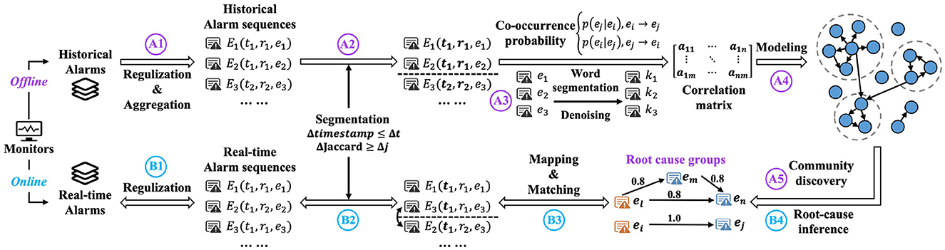
Figure 1. The overview of communication alarm analysis framework.

2.1. The offline learning procedure

Figure 1 (A1 to A5) shows the offline learning process, and it consists of the following five steps (A1) Pre-process, collecting historical alarms from monitors for a specific period as offline training data, such as a set of data before the alarm occurs. Then, filter and regulate alarm attributes based on human-designed rule templates, reorganize alarm sequences of the same or similar sources that occur in a short interval, and output a regulated historical alarm sequence. (A2) Segmentation of historical alarm sequences based on alarm time and alarm sources. The outputs are segments of alarm sequences for different alarm scenarios. (A3) Historical alert association mining, including alert association based on context and content, both are represented by an association matrix. Context associations are obtained by constructing a co-occurrence probability model, and content associations are obtained by calculating content similarity. The outputs are historical alarm association matrices. (A4) A directed and acyclic probabilistic graph is constructed based on the historical alarm association matrices as an alarm association model. (A5) The association noise is eliminated by the community discovery algorithm, and the closely associated alarm groups are classified as association reduction results of offline learning and further used for online analysis.

2.2. The online analysis procedure

Figure 1 (B1–B4) shows the online analysis process, and it consists of the following four steps: (B1) Real-time alarm collection and pre-processing collect alarms from monitors with a fixed time interval and regulate them in the same way as offline learning. (B2) Aggregate and reorganize alarms based on data sources and divide them into segments. The outputs are segments of alarm sequences in different scenarios. (B3) Real-time compression by alarm matching matches alarms within each segment based on the results of offline learning. The matched alarms are separated according to the grouping result of offline learning, while the unmatched alarms are constructed into similar sets based on historical alarms. Finally, the alarms are placed into different groups. (B4) Calculate and rank the importance of the alarms in matched compression groups. The alarm with the highest score is marked as the root cause. Meanwhile, the root cause of the corresponding group information is reported to network operators.

3. Offline learning of communication network alarms

3.1. Alarm sequence segmentation

3.1.1. Definition

Alarm Scenarios and Failure Scenarios. As shown in Figure 2A, communication networks are deployed in different and independent areas, and alarms propagate in the same or neighboring machine rooms. Therefore, we define Alarm Scenarios when alarms are generated within a short interval and at the same or similar data sources (i.e., machine rooms hosting the communication devices), and the propagation of alarm in the same scenario is defined as a Fault Scenario. We further count the time interval of alarms in a month based on the real communication networks, as shown in Figure 2B. The alarms that belong to the same propagation and appear within 1 min account for more than 95%. It indicates that alarms propagate fast, and when the time interval is more than 1 min, there is a low association between alarms. According to the above results, we set the segmentation threshold of the alarm sequence as 1 min.

FIGURE 2

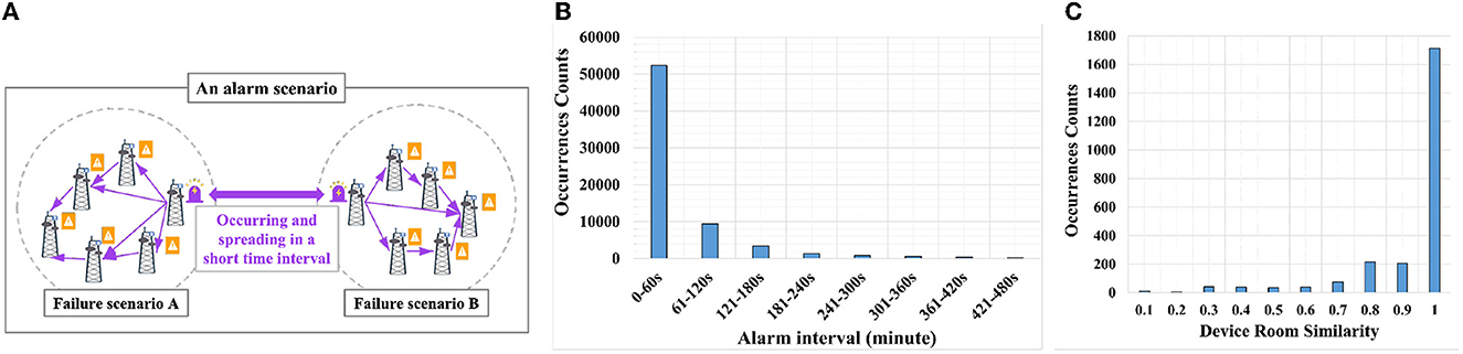
Figure 2. The definition and statistical results. (A) Example of alarm scenario and failure scenario. (B) Alarm time interval histogram. (C) Statistical counts of similarity of alarm device room.

Additionally, because there are numerous alarms within 1 min, segmentation only based on time threshold may classify redundant and inaccurate sequences belonging to different alarm scenarios. Therefore, we counted the characteristics of other attributes of related alarms, such as the similarity of the data sources (e.g., device room), as shown in Figure 2C, more than 70% of the associated alarms occur in the same room site, and 20% in neighboring room sites (similarity values from 0.7 to 1.0). There are also room sites with low similarities, which are affected by inaccurate descriptions and biased data labels in the similarity calculation. Furthermore, cross-site propagation exists in real environments, but such cases are very scarce, and setting a low similarity threshold in sequence segmentation will result in incorrect segmentation. Therefore, we do not consider corner cases such as cross-site propagation and select 0.6 as the scenario segmentation threshold.

3.1.2. Alarm sequence segmentation algorithm

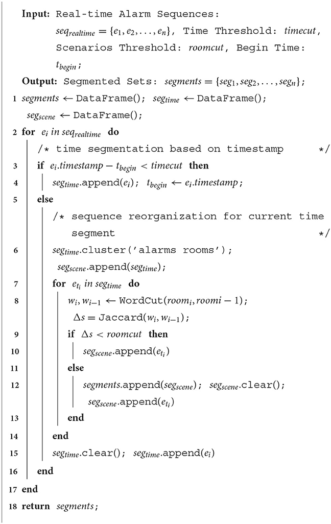
According to the above analysis, alarms of the same scenario usually occur within 1 min and appear in the same or close to the occurrence room site. Based on the similarity of occurrence time and the occurrence room, the segmentation algorithm is defined as Algorithm 1 (O(n) time complexity). Figure 3A shows an example of the alarm segmentation results.

ALGORITHM 1

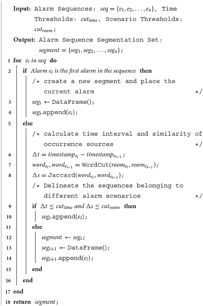
Algorithm 1. Alarm sequence segmentation algorithm.

FIGURE 3

Figure 3. The segmentation algorithm and sequence patterns. (A) Example of alarm sequences segmentation. (B) Example of base station alarm sequence pattern.

3.2. Alarm association mining

The alarm sequence segmentation algorithm separates alarm sequences of different alarm scenarios, but we need further root cause analysis of alarms in one scenario. As shown in Figure 2A, two different root cause alarms (marked by alarm icons) occurred at a similar time and in nearby sites, causing other alarms (marked by warning icons). Thus, alarms within different fault scenarios have different propagation paths, and alarms of the same fault scenario are highly correlated. Therefore, after sequence segmentation, it is necessary to divide alarms into different fault scenarios and infer their propagation paths.

Based on the analysis of real alarm data, alarms with the same root cause usually have a high probability of co-occurrence (Weng et al., 2018). Moreover, the related alarms show similarity in attributes such as room sites, device, and alarm content (Zhao et al., 2020). As for the device association, it is difficult to obtain the exact topology due to the complex dependencies of communication network devices and components in real production. Currently, widely used spatial analysis methods such as topological network construction and topological region delineation rely on accurate topology, and inaccurate topological knowledge generates more noise. Therefore, (i) for the spatial association of communication network alarms, we mainly consider the association between the alarm sources in the sequence segmentation process. (ii) For the association of alarm contents, we mainly consider the title of crucial alarms because of the redundant information in alarm details. Table 1 shows examples of related alarms, which have similar titles. Furthermore, analyzing their similarities can supplement the shortage in context association. However, there are redundant content or abbreviation irregularities in alarm titles, which need to be standardized in pre-processing.

TABLE 1

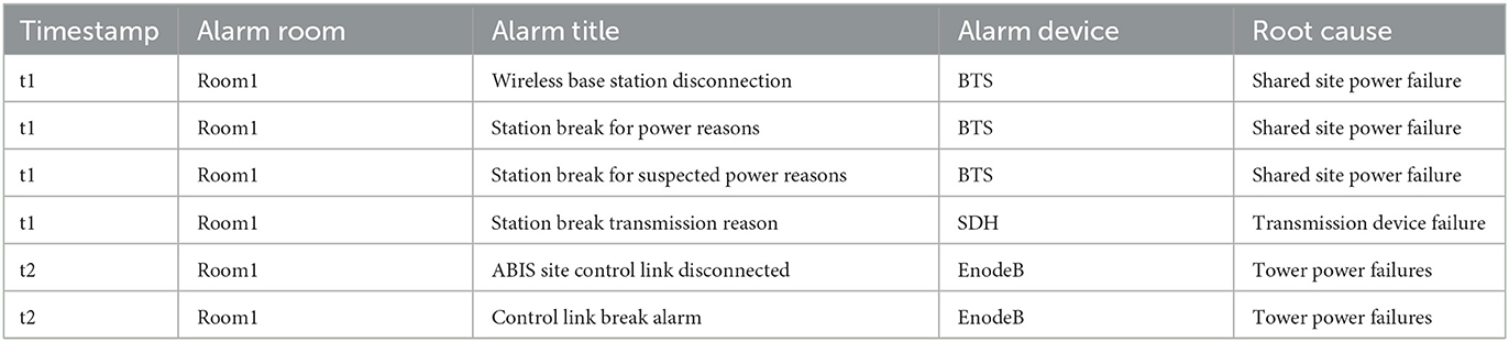
Table 1. Example of associated alarms.

3.2.1. Association of alarm context

Alarms in real communication networks are usually not periodic, and the frequency of occurrence varies widely. We collected the real alarm data from a telecom operator in a month. The data show that frequent alarms are as many as thousands, while scarce alarms are only a few. In addition, numerous alarms occur at the same time, and their timestamps are susceptible to deviations due to external factors, resulting in unstable alarm sequences and difficulty in capturing a uniform sequence pattern, as shown in Figure 3B. Therefore, association mining algorithms based on frequent or sequential patterns, such as the Apriori algorithm (Bodon, 2000), FP-growth algorithm (Borgelt, 2005), WINEPI algorithm (Li et al., 2010), and PrefixSpan (Han et al., 2001) algorithm, have difficulty in extracting the association of non-periodic or episodic alarms. In neural network-based association mining, irregular sequences can seriously affect the training effect of models. To adapt to irregular and non-periodic alarms, we construct a novel probabilistic model to mine context association of alarms, which is based on the Bayesian theory (Bernardo and Smith, 2009), using statistical learning (Vapnik, 1999) instead of prior knowledge, defined as Equation (1).

$\begin{array}{l}D(e_i,e_j)=\\ \{\begin{array}{l}P(e_j|e_i)\text{\hspace{1em}if Count}{(e_i\to e_j)}_{e_i,e_j\in se{g}_k}\ge \text{Count}{(e_j\to e_i)}_{e_i,e_j\in se{g}_k}\hfill \\ P(e_i|e_j)\text{\hspace{1em}if Count}{(e_i\to e_j)}_{e_i,e_j\in se{g}_k}<\text{Count}{(e_j\to e_i)}_{e_i,e_j\in se{g}_k},\hfill \end{array}& (1)\end{array}$

where D(e_i, e_j) denotes the co-occurrence probability of alarms e_i and e_j. To obtain the alarm propagation paths, conditional probability is used to represent the alarm co-occurrence probability. However, it is difficult to obtain the propagation paths of alarms in real communication networks. We obtain it based on statistical learning, summarizing the directions of co-occurrence alarms in a segment. Thus, Count(_{ei → ej)ei, ej∈segk} denotes the count of alarm e_i occurs before e_j in segment seg_k, and the opposite is defined as Count(_{ej → ei)ei, ej∈segk}. When alarm e_i precedes e_j more times in a segment, the co-occurrence probability is expressed as conditional probability P(e_j|e_i). The mathematical meaning is the occurrence probability of alarm e_j under the condition that alarm e_i occurs and vice versa for P(e_i|e_j). Equation (2) is a calculation example of conditional probability P(e_j|e_i).

$\begin{array}{l}P(e_j|e_i)=\\ \{\begin{array}{ll}\max \left(\frac{\text{Count}{(e_i|e_i,e_j)}_{e_i,e_j\in se{g}_k}}{\text{Count}(e_i)},\frac{\text{Count}{(e_j|e_i,e_j)}_{e_i,e_j\in se{g}_k}}{\text{Count}(e_j)}\right)\hfill & \text{if Δ}c\le \text{Δ}d\hfill \\ \frac{\text{Count}{(e_i|e_i,e_j)}_{e_i,e_j\in se{g}_k}+\text{Count}{(e_j|e_i,e_j)}_{e_i,e_j\in se{g}_k}}{\text{Count}(e_i)+\text{Count}(e_j)}\hfill & \text{if Δ}c>\text{Δ}d\hfill \end{array}& (2)\end{array}$

$\begin{array}{l}\text{Δ}c=|\text{Count}(e_i)-\text{Count}(e_j)|,\text{Δ}d\text{ is a hyperparameter threshold},\\ \end{array}$

where Count(e_i|e_i, e_j) and Count(e_j|e_i, e_j) are the number of alarms e_i and e_j in a single segment. Count(e_i) and Count(e_j) are the total number of e_i and e_j in all segments. Δc is the absolute value of the difference between alarms e_i and e_j. Δd is a hyperparameter threshold determining whether the frequency of alarms is different from each other. According to the co-occurrence of associated alarms, (i) for two alarms with a small difference in the count, the conditional probability is the larger value (the proportion of co-occurrence to each count). When the propagation direction is uncertain, choosing the maximum value can remain the association when the noise is removed. (ii) as for two alarms with a significant difference in the occurrence count. To avoid the effect of episodic alarms, conditional probability is defined as the count of co-occurrence alarms in a segment divided by the total count of two alarms. The threshold Δd is a statistical count value of alarms within a certain period, we set Δd = 370 in our experiments, which is the average count within a month.

3.2.2. Association of alarm content

The offline learning procedure is based on the historical data of a certain period that may have potential errors. To ensure the accuracy of association mining, further analysis is needed with other attributes of alarms. We mainly consider the similarity between alarm titles, but according to Table 1, titles need to be regulated first. We collect professional terms for communication network alarm events to extend the Chinese Thesaurus (jieba, 2020). Then, alarm titles are sorted according to the occurrence of count of words in descending order as two types. (i) Keywords, such as “withdrawal, broken link, broken station”. (ii) Normal words, such as “occurrence, of” and variables such as interface and address number. We generate a list of key terms for alarms based on expert experience and a list of synonym conversions, such as “LOS” equals “loss of signal”. Table 2 shows an example of the processing of alert titles, and it shows that the irregularities come from normal words and synonyms. Therefore, we regularized the titles by subdividing and filtering them using synonym lists and keyword lists. After regularization, the similarity of alarm titles can be better calculated. Considering the word shifting and repetition in regularization, we choose the Jaccard coefficient (Niwattanakul et al., 2013) to calculate the similarity, defined as Equation (3).

$\begin{array}{ll}S(e_i,e_j)=\text{Jaccard}(tex{t}_i,tex{t}_j)=\frac{\text{keyword}(tex{t}_i)\bigcap \text{keyword}(tex{t}_j)}{\text{keyword}(tex{t}_i)\bigcup \text{keyword}(tex{t}_j)}& (3)\end{array}$

TABLE 2

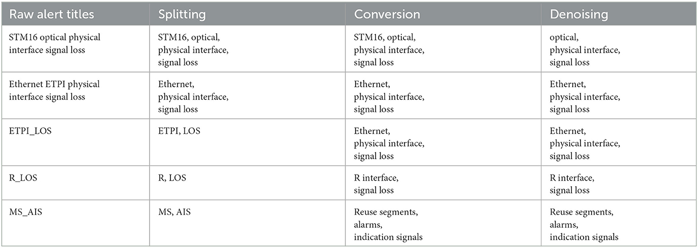
Table 2. Examples of the alert title processing.

3.2.3. Construction of association matrix

The association N × N matrix, where N is the number of historical alarms, is constructed based on context association and content association of alarms according to Equation (4). The hyperparameter α ∈ [0, 1] is an association weight, which is a trade-off on the importance between context and content. Generally, if the alarm sequence patterns are straightforward, we could concentrate on the context and set a larger α. In this study, we set α = 0.6 with more attention to the context association and regard content association as additional information.

$\begin{array}{ll}{\text{Cov}}_{e_i,e_j}=\alpha \times D(e_i,e_j)+(1-\alpha )\times S(e_i,e_j)& (4)\end{array}$

3.3. Alarm reduction based on association

Figure 4A shows the cumulative distribution of the values in association matrices, where the lower values are the noise. They have weakly associated alarms with the same time or occurrence sites but are triggered by different root causes. The noise usually belongs to different failure scenarios that can be filtered out using co-occurrence probabilities. For the preprocessing of denoising, threshold filtering is widely used (Marvasti, 2015). However, it is difficult to set a proper threshold for real communication network alarms, and the filtering accuracy is unacceptable. Larger thresholds may lose important associations, and smaller thresholds fail to filter noises. In contrast, clustering or community discovery (Coscia et al., 2011) is more feasible. Meanwhile, the clustering algorithm still requires hyperparameters such as the number of centers in K-means (Hartigan and Wong, 1979) or distance of DBSCAN (Ester et al., 1996). Therefore, we turn to the non-parametric Louvain community discovery algorithm (De Meo et al., 2011), which is measured by the metrics of association grouping results.

FIGURE 4

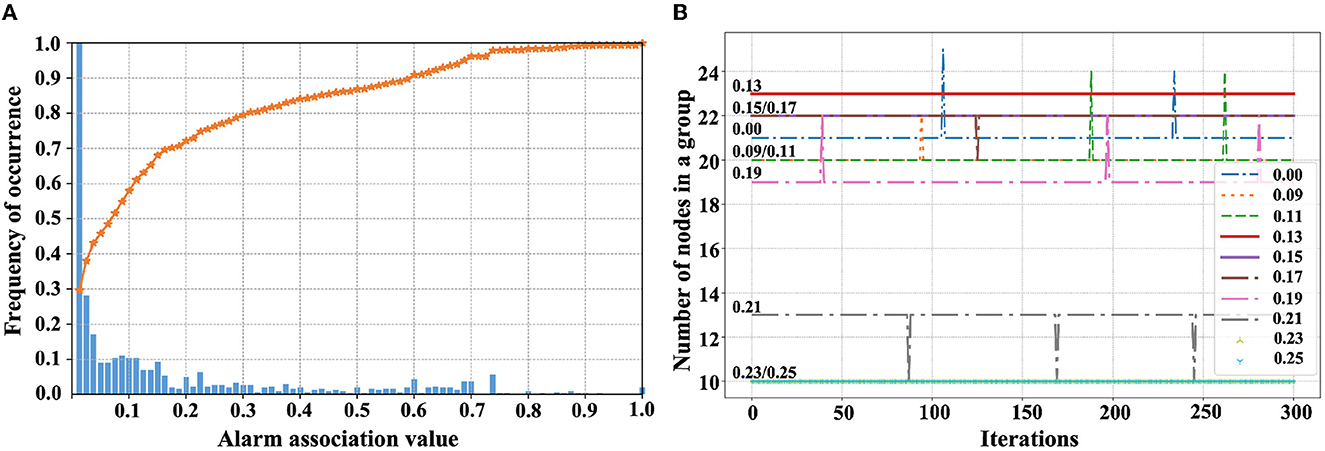
Figure 4. The statistical results and threshold comparison. (A) Statistical histogram of alarm correlation values. (B) Comparison of different denoising threshold.

The association of communication network alarms is modeled by a directed acyclic graph (DAG), where the nodes are alarms, the directed edges denote the propagation direction of alarms, and the weights of the edges are association levels. Then, the community-based discovery algorithm finds out associations from the graph as reduction results. Since it is a directed graph, we add weights to module metrics, defined as Equation (5), where G denotes an undirected graph converted from the directed association graph. We ignore the propagation direction because our reduction mainly considers the degree of association. Moreover, C(C ∈ G) denotes a community, ∑ Cov(_{ei, ej)ei, ej ∈ G} denotes the sum of all edge weights in the graph G, ∑ Cov(_{ei, ej)ei, ej ∈ C} denotes the sum of all edge weights of community C, and ∑ Cov(_{ei, ej)ei ∈ C, ej ∈ G} denotes the sum of associated edge weights of community C. Based on Equation (5), the community with the largest module degree Q is the closest alarm association.

$\begin{array}{ll}Q=\sum \left(\frac{\sum \text{Cov}{\left(e_i,e_j\right)}_{e_i,e_j\in C}}{\sum \text{Cov}{(e_i,e_j)}_{e_i,e_j\in G}}-{\left(\frac{\sum \text{Cov}{(e_i,e_j)}_{e_i\in C,e_j\in G}}{2\times \sum \text{Cov}{(e_i,e_j)}_{e_i,e_j\in G}}\right)}^2\right)& (5)\end{array}$

The Louvain algorithm visits communities randomly, and a large number of graph edges may lead to biased division. Therefore, eliminating invalid associated edges can improve the accuracy and stability of reduction. We set different reduction thresholds by locating the alarm nodes that are inconsistent in multiple divisions. We count the number of nodes in a group, and when the number is stable in multiple iterations, the invalid edges affecting the reduction are eliminated. As shown in Figure 4B, the deviations generated by the invalid edges are small, and stable groups are obtained in the iterations when the reduction thresholds are [0.13, 0.15, 0.23, and 0.25]. Therefore, we set 0.13 in our experiments. The association reduction algorithm is shown in Algorithm 2 (O(n²) time complexity), including association denoising and community discovery, and finally generates the groups of associated alarms.

ALGORITHM 2

Algorithm 2. Association reduction algorithm.

4. Online analysis of communication network alarms

4.1. Real-time alarm compression

The real communication network alarms are numerous even millions when an alarm storm occurs. Moreover, their occurrences are unstable, leading to difficulty in setting a fixed time window for analysis (Hu et al., 2017). Inappropriate time window results in incorrect classification results of alarms. Therefore, we propose a real-time sequence segmentation (Algorithm 3) (O(n²) time complexity) based on offline learned alarm associations to group alarms, then analyze them by groups. There are three steps as follows: (i) the associated alarms are segmented by the interval threshold at first. (ii) Reorganize sequences within the same time segment according to alarm sources (machine rooms or device names) and aggregate alarms with the same or similar sources. It can reduce the impact of timing deviations and enhance the alarm compression rate. (iii) Based on the aggregation results and the reorganized sequences, dividing alarms into different alarm scenarios for subsequent analysis.

ALGORITHM 3

Algorithm 3. Real-time alarm segmentation.

Alarms are further divided into matched and unmatched alarms based on historical data. We propose the real-time alarm matching and compression algorithm as shown in Algorithm 4 (O(n²) time complexity). (i) Matched alarms are events that appear in offline learning, which are grouped using the association reduction results. This matching is based on the list of compressed alarm association groups. If the current alarm groups have a majority intersection with the group list of a compressed collection, it can be put into that collection. (ii) The unmatched alarms are mainly new types of alarms or independent alarms, which are grouped by the similarity to historical alarms. We extract the key contents of the current alarm and calculate its similarity with historical alarms, then sort them in descending order and form a similar set as the historical alarms with Top-k similarity. If the alarm belongs to a compressed segment in a similar set, it will be put into that group. Otherwise, the alarm is put into the independent groups. (iii) Finally, new alarms with a low similarity are grouped into an independent group.

ALGORITHM 4

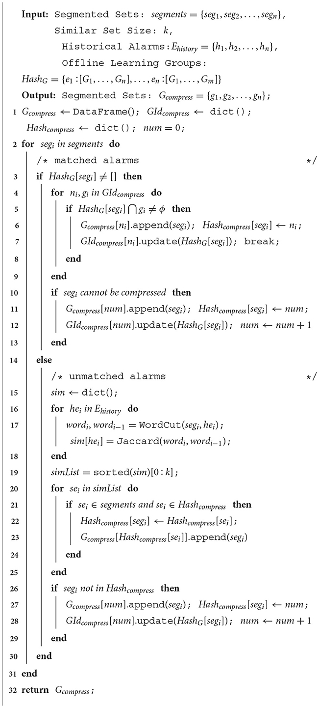
Algorithm 4. Real-time alarm matching and compression.

4.2. Root cause inference

When an alarm storm occurs, there are still numerous compressed alarm groups. Automatically inferring the root cause is necessary. In communication networks, the root cause alarm results in a wide propagation scope but is nearly not influenced by other nodes. Therefore, root cause alarms usually have more out-degree edges (and out-degree weights) and fewer in-degree edges (and in-degree weights) in the association graph. To infer the root cause alarm, we modify the PageRank algorithm to obtain importance scores. PageRank is a basic algorithm for evaluating the importance of a website and is applied to identify the key nodes (Tortosa et al., 2021; Xiong and Xiao, 2021). Our improved PageRank algorithm not only considers the number of in and out edges but also incorporates weights to calculate the importance score. Based on the association graph shown in Figure 5A, for in-edges, the importance of node e_i on node e_x in Figure 5 (a2) is greater than in Figure 5 (a1). For out-edges, the importance of node e_x influenced by node e_i in Figure 5 (a2) is greater than in Figure 5 (a3). In summary, for alarm node e_i, : the meaning of the sentence “In summary, for alarm node ei....” is not clear. Please check and confirm whether this sentence is appropriate or amend if necessary. define the importance of impact as $In{f}_{imp(e_i)}^{+}$ and the importance of being impacted as $In{f}_{imp(e_i)}^{-}$, as shown in Equation (6), where OutSet(e_i) and InSet(e_i) are the set of out-degree and in-degree of alarm node e_i. PR is the original definition of node importance in the PageRank algorithm.

$\begin{array}{l}In{f}_{imp(e_i)}^{+}={\displaystyle {\sum }_{e_k\in OutSet(e_i)}\frac{PR(e_k)}{\text{InDegree}(e_k)},}In{f}_{imp(e_i)}^{-}\text{ =}\\ {\displaystyle {\sum }_{e_j\in InSet(e_i)}\frac{PR(e_j)}{\text{OutDegree}(e_j)}}& (6)\end{array}$

FIGURE 5

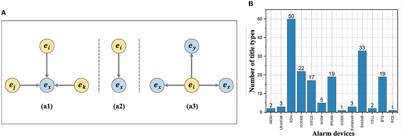
Figure 5. The importance example and statistical results of alarm devices. (A) Example of impact importance of node. (B) Statistical results of alarm title types on each device.

We further consider the association weight of alarms to indicate the impact degree and the larger value means a greater impact. Adding weights not only quantifies the impact degree but also accelerates the convergence of the algorithm. Therefore, we define a new importance of impact as Equation (7), where $Inf{(e_i)}^{+}$ and $Inf{(e_i)}^{-}$ denote the importance of impact and being impacted of alarm node e_i.

$\begin{array}{ll}\begin{array}{c}Inf{(e_i)}^{+}={\displaystyle \sum _{e_k\in OutSet(e_i)}}\frac{PR(e_k)}{\text{InDegree}(e_k)}\times Co{v}_{e_i,e_k},\\ Inf{(e_i)}^{-}={\displaystyle \sum _{e_j\in InSet(e_i)}}\frac{PR(e_j)}{\text{OutDegree}(e_j)}\times Co{v}_{e_j,e_i}\end{array}& (7)\end{array}$

We also modify the definition of PR (node importance score in PageRank), which is the relationship of the influence degree of one node on rest nodes, as shown in Equation (8). Therefore, the node with the highest importance score is the most likely root cause node.

$\begin{array}{ll}PR(e_i)=Inf{(e_i)}^{+}-Inf{(e_i)}^{-}& (8)\end{array}$

Based on the above definitions, we propose a root cause inference (Algorithm 5) (O(n²) time complexity) to infer root cause alarms in grouped alarm sets. The algorithm includes initialization, iterative update, and importance ranking. Moreover, the root cause node is output when it reaches a stable distribution.

ALGORITHM 5

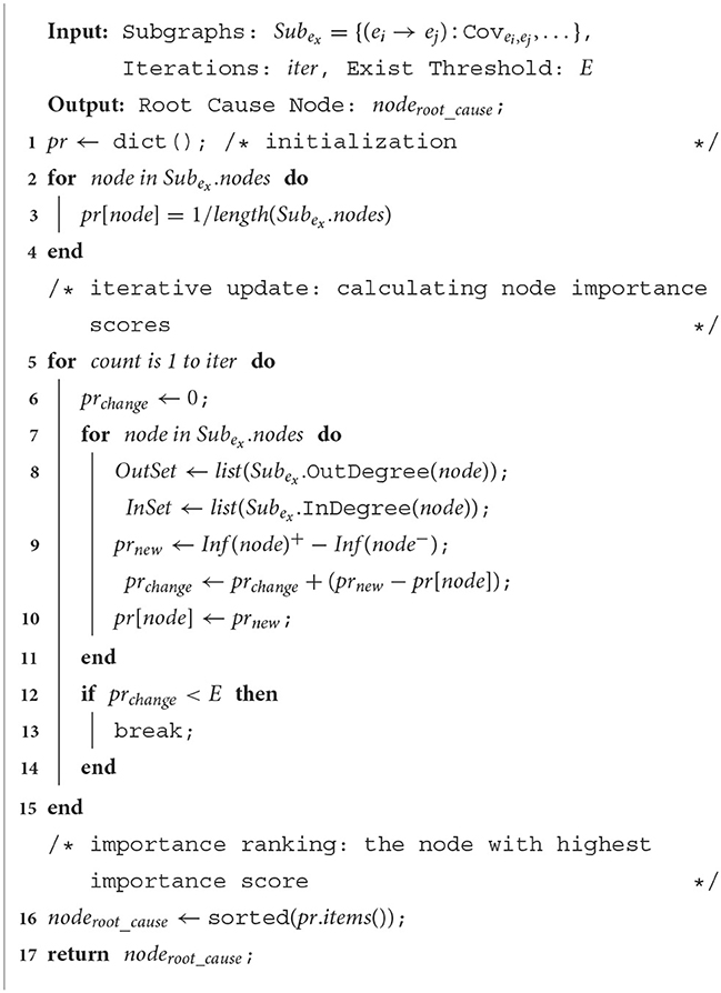
Algorithm 5. Alarm sequence segmentation algorithm.

5. Evaluation

5.1. Dataset

Our dataset comes from a real-world telecom operator's real communication network, and it contains real alarms from June 1st to 30 in 2019, with a total of 154, 273 alarm records, of which 12, 253 are grouped and labeled by experts. We use data from June 1st to 22 as training data for offline learning and obtain association reduction results. Then use labeled data from June 23 to 30 for online analysis testing.

5.1.1. Regularization and preprocessing

We regularized the communication network alarms by extracting a uniform template. To reduce the interference of invalid information, only attributes that are valid for analysis are retained. According to our alarm sequence segmentation and association analysis, we select the following attributes including occurrence time, machine room, alarm title, device type, network element name, and alarm level. We count the categories of the above attributes on the training dataset, which contains 13 categories of device types, 144 categories of alarm titles, and 12, 201 categories of network element names. Therefore, we discard the network element name attribute because it is too fine-grained compared to the others, it is not conducive to alarm association analysis.

We further analyze the alarm titles on each device, as shown in Figure 5B, most of the alarm contents occur on specific devices. Therefore, we define two types of regular alarm templates. (i) Alarm template based on alarm titles, we define the regular alarm event as $e_i^{ind}=\left\{a_i\right\}$ and a regular alarm record as $E_i^{ind}=\left\{a_i,t_i,r_i,g_i,l_i\right\}$. Alarms with the same title are regarded as the same alarm event. (ii) Alarm template based on the alarm title and device attributes, we define the regular alarm event as $e_i^{mix}=\left\{a_i,d_i\right\}$ and a regular alarm record as $E_i^{mix}=\left\{a_i,d_i,t_i,r_i,g_i,l_i\right\}$. Alarms with the same title and device type are regarded as the same alarm event. In the above definitions, where t_i is the timestamp, r_i is the alarm room, a_i is the alarm title, g_i is the alarm level,l_i is the alarm label, d_i is alarm device. Our analysis framework mainly uses the second rule template $e_i^{mix}$.

Due to the influence of external factors such as network delay or system clock offset, there are inaccuracies in timestamps. To deal with this problem, we set a time window and treat alarms in a window as occurring at the same timestamp. Alarm scenario aggregation reorganizes the alarms that occur at the same time according to alarm sources and improves the compressibility of the alarm sequence. We set the time window as one minute based on our statistical summarizing in Section 3.1, most of the relevant alarms occur within one minute. Based on the raw training dataset, the historical sequence segmentation algorithm can obtain 33, 968 segments. However, after scenario aggregation, the number of segments further reduces to 23, 798, which reduces 30% of segments, effectively improving the compression rate of the alarm sequence.

5.2. Evaluation of offline learning

We mainly validate the compression results of offline learning. It starts with historical sequence segmentation of the regulized and scenario-aggregated training data with 23, 798 segments (Algorithm 1). Then, the association matrix is constructed by mining contextual dependencies and content similarity of alarm segments. The alarm association is constructed as a probabilistic-directed acyclic graph. Moreover, a total of 169 nodes with 391 associated edges are generated based on the training data, which is shown in Figure 6A. The noisy association causes a large number of ungrouped alarms which cannot be used for analysis. The area marked by purple circles in Figure 6A are grouped alarms. The association graph is analyzed using the association reduction (Algorithm 2) and root cause inference (Algorithm 5). We obtain 169 reduced association groups, Figure 6B shows part of the results, where the purple nodes are the root cause alarms of corresponding groups. It shows that our offline learning procedure eliminates noises from historical alarm association graphs and further makes alarm grouping more accurate.

FIGURE 6

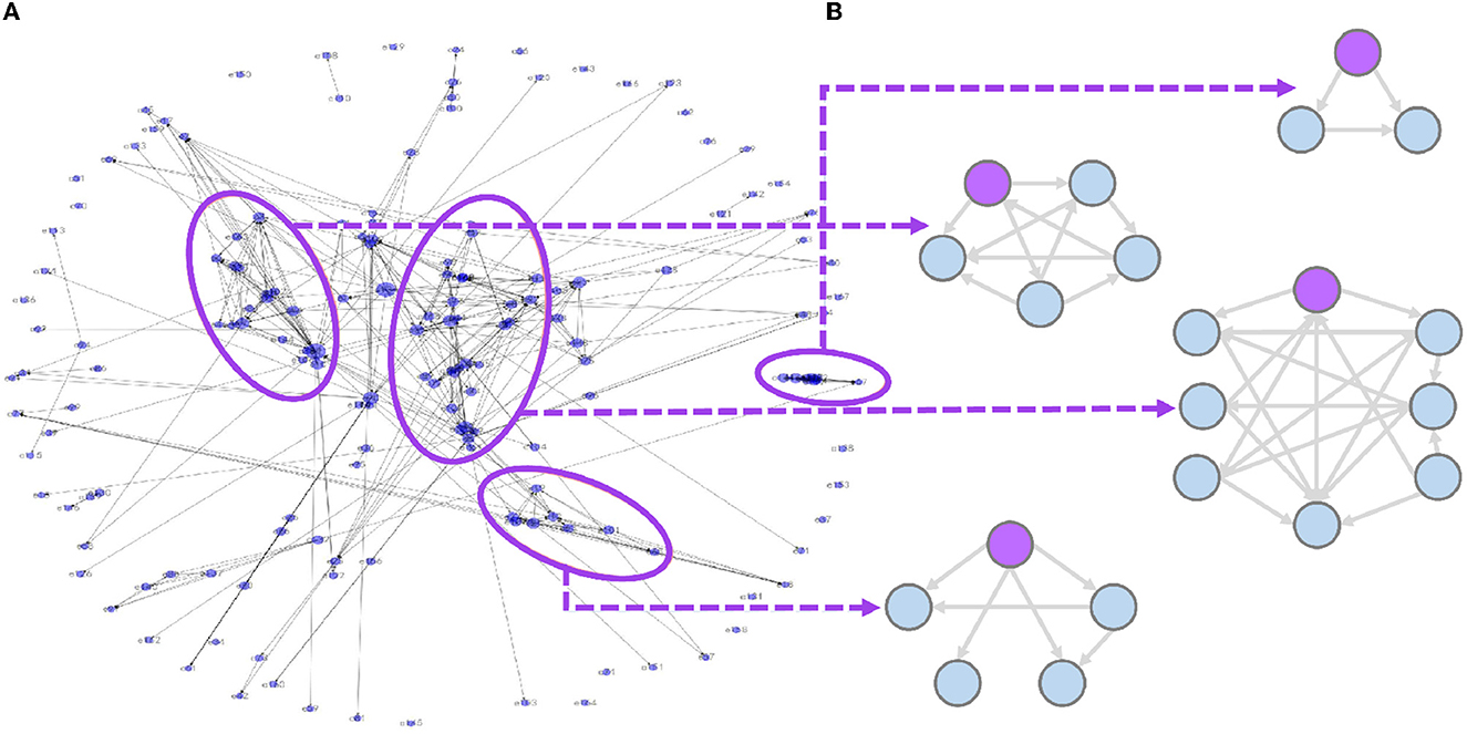
Figure 6. Example of association reduction in offline learning procedure. (A) Original alarm association. (B) Example of alarm groups.

5.2.1. Online compression

Online compression is based on the results of offline learning. In addition, we generate real-time alarms based on the test dataset to validate the effectiveness of online compression. After data preprocessing, the real-time alarm segmentation (Algorithm 3) and the real-time alarm compression (Algorithm 4) are used for compression. The compression rate can reach up to 40%. Figure 7 shows an example of the compression results. The left part shows a real-time alarm sequence obtained in a segment. The right part shows the analysis results, where the nodes marked in purple color at the top are inferred root causes of the group. Meanwhile, the edges which are highly correlated with root causes are denoted by dark arrows, while other edges are denoted by lighter arrows. It shows that our online analysis effectively compresses the alarms and infers the propagation of key root causes in the compressed group.

FIGURE 7

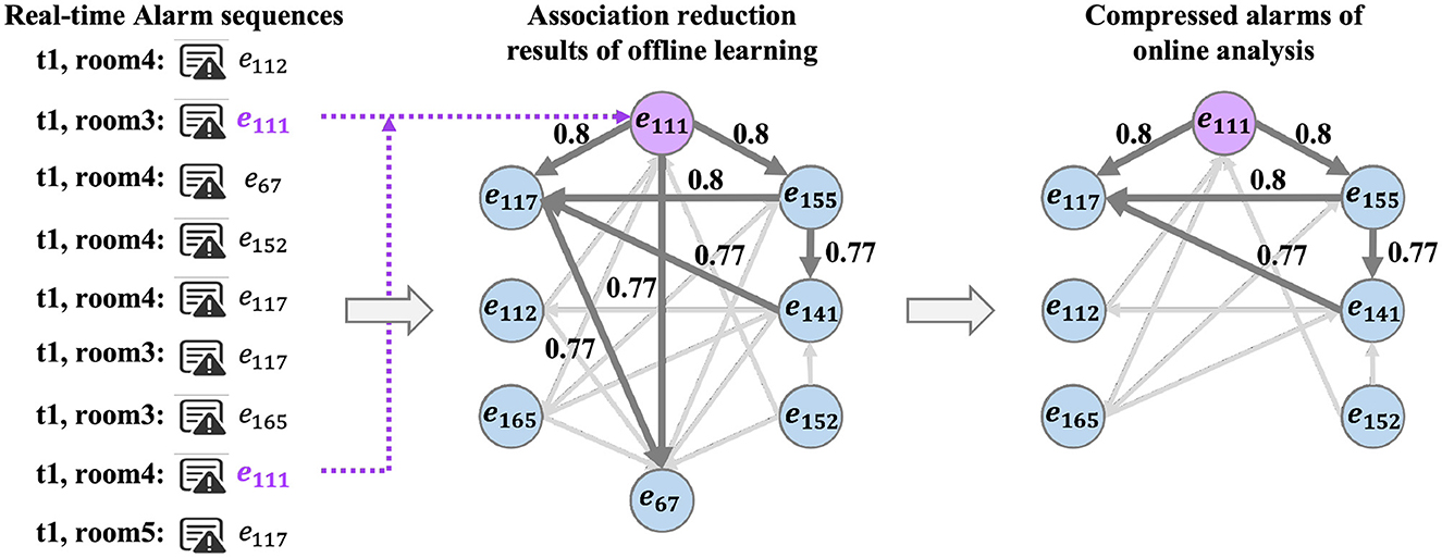
Figure 7. Example of real-time alarm mapping matching.

5.3. Evaluation of online analysis

5.3.1. Metrics

We define three key metrics to evaluate our alarm analysis results.

(i) Alarm loss. We define “lost alarms", which are independent alarms and not associated with other alarms and are usually filtered out as noises. This idea comes from two aspects. One is about the truly independent alarms, and the other is about failing to extract the associations from alarms due to improper association analysis methods. Since the number of independent alarms is fixed, the number of lost alarms can evaluate the capability of analysis algorithms. The alarm loss is defined as $eventLoss=\frac{even{t}_{loss}}{\sum even{t}_{all}}$, where event_loss are independent nodes and ∑ event_all is the total number of alarms. The smaller eventLoss indicates a more comprehensive mining of the method.

(ii) Group accuracy. It is defined as $accuracy=\frac{TruePositive}{totalalarms}$, and the higher accuracy indicates the more reliable association reduction and matching results of the analysis method. The true positive is evaluated based on the dataset labeled by experts.

(iii) Compression rate. It is the compression degree of the number of alarms, defined as $compress=\frac{alarms-groups}{alarms}$, where alarms is the total number of alarms, and groups is the number of groups. A higher compression rate means a greater compression degree of alarms.

5.3.2. Regularization and pre-processing

We compare the results of the two regularization templates, as shown in Table 3, where e^ind is a template only based on alarm titles, and e^mix is a fine-grained template based on alarm titles and device attributes. Scenario aggregation refers to the reorganization of alarms with similar occurrence sources in the pre-processing phase. The results in Table 3 show that scenario aggregation not only improves the grouping accuracy but also effectively improves the compression rate. In addition, different templates have less impact on compression but some impact on grouping accuracy, among which templates e^ind based on alarm titles achieve better results. Because of the fineness of the alarm labels in the test dataset, which is only labeled at the title level.

TABLE 3

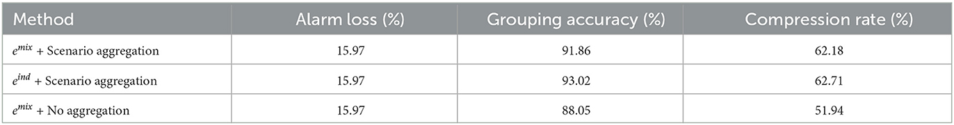
Table 3. Comparison of regularization and pre-processing methods.

5.3.3. Association analysis of alarms

We compare several commonly used alarm association analysis methods in communication networks. (i) Frequent pattern mining methods, such as improved Apriori algorithm (Bodon, 2000) and FP-Growth algorithm (Borgelt, 2005). (ii) Sequence pattern mining methods, we choose the PreFixSpan algorithm (Han et al., 2001), which is widely applied in the field of alarm analysis. (iii) Neural network-based methods, we chose the LSTM model (Yu et al., 2019) to learn the sequence relationship for predictive analysis, and the input is the unique encoding (one-hot) of the warning sequence. (iv) Word embedding-based methods, which convert alarm sequences into word sequences for analysis. It is one of the most effective analysis methods in recent years, and we choose the word embedding-based (Li et al., 2018) APE interaction model (Paradis et al., 2004) for comparison.

We compare the above models in extracting association relationships based on the training dataset and then use the test dataset to validate their association analysis results. Table 4 shows the optimal results of each method. We summarize as follows: (i) the Apriori algorithm and FP-Growth algorithm can only capture the association of frequently occurring alarms and lose a large number of non-periodic or episodic alarms, which seriously affects the grouping accuracy and compression rate. (ii) The PreFixSpan algorithm can only capture alarm association with fixed sequential patterns and loses alarm with sequential deviations and non-periodic ones. It has a certain improvement over the frequent pattern mining methods. (iii) The LSTM-based model predicts alarms based on the prior sequence and does not have the problem of alarm loss. However, the irregularity of communication network alarms and the diversity of sequences lead to costly training and low prediction accuracy. Meanwhile, the model cannot determine the alarm propagation direction as well as perform alarm compression, so we only record the accuracy rate. (iv) The APE model is also unable to determine the propagation direction and needs to calculate between each pair of alarms, which includes a large number of redundant calculations. The reduction process also costs a long time and it is weak to eliminate association noise. Our method performs better on all metrics. It not only mines the association relationship with fixed pattern alarms but also non-periodic and episodic alarms. Therefore, it can provide more accurate and reliable association reduction results, compress massive real-time alarms, and accelerate analysis.

TABLE 4

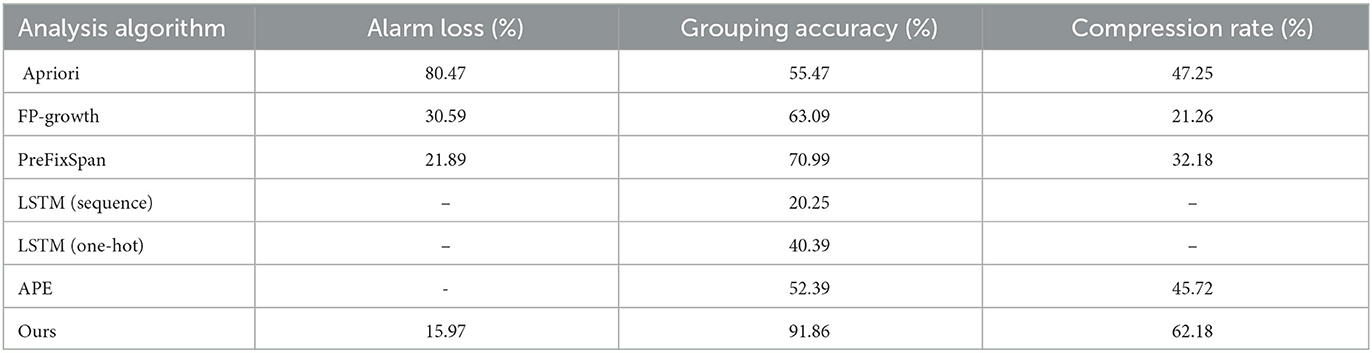
Table 4. Comparison of association analysis algorithm.

5.3.4. Association reduction results

Figure 8A shows a representative case of two groups. The left and right parts of the graph are divided into two closely correlative subgroups. The value of the connected edge (marked in red) between the two subgroups is much lower than the average value within the two groups, thus it is regarded as an association noise. However, since the noisy edge weights cannot be known in advance, the ability to eliminate the noise is limited by setting proper thresholds and clustering distance. Three popular community discovery algorithms are compared in Figure 8, namely (a) the Infomap algorithm (Rosvall and Bergstrom, 2008), (b) the LPA algorithm (Zhu et al., 2003), and (c) the Louvain algorithm (De Meo et al., 2011). As shown in Figure 4, only the Louvain algorithm eliminates the noisy edge of the subgraph and correctly divides the groups. The LPA algorithm incorrectly eliminates associations and obtains 6 groups. The Infomap algorithm does not correctly identify the noisy edge. We further selected the threshold value 0.2 (CDF curve inflection point value) for comparison based on the results of the association statistics value as shown in Table 5. The threshold-based graph reduction method has unstable grouping accuracy, and the LPA algorithm loses important relations and performs poorly in grouping accuracy and compression rate. The Infomap algorithm has poor elimination of noises and poor effectiveness. The Louvain algorithm performs the best in both grouping accuracy and compression rate and eliminates noises more comprehensively.

FIGURE 8

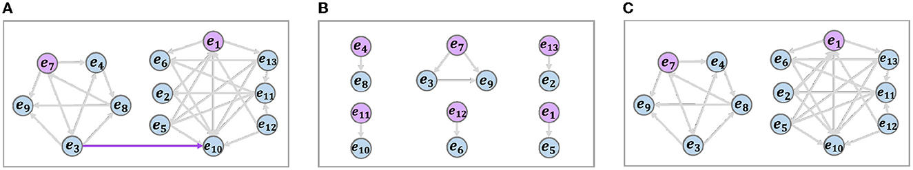
Figure 8. Association reduction results of different algorithms. (A) Origin and infomap. (B) LPA. (C) Louvain.

TABLE 5

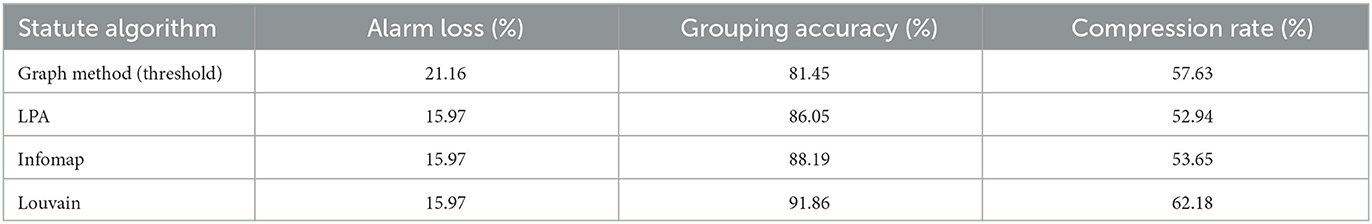
Table 5. Comparison of association statute algorithm.

5.3.5. Real-time matching and compression

Real-time alarm matching and compression (Algorithm 4) include matching alarm groups based on offline learning and grouping unmatched ones based on similarity. As the expert-tagged alarms dataset does not contain unmatched alarms. To expand the dataset, we use the expert-labeled test dataset to form eliminable alarms set Alarm_remove = {e_r1, …, e_rn} and simulate the unmatched alarms. Those alarms mainly consist of independent alarms and new alarms that do not appear in history, both of which are rare in general. The number of independent alarms is <15% of the total alarms. The number of new alarms is estimated by calculating the proportion of alarms that occur in the last 3 days and not in the first 7 days based on the real alarm data with a 10-day period, which is <5% of the total. Our experiments eliminate the alarms one by one in Alarm_remove from the training dataset sequentially, and the results are shown in Table 6. The impacts of different proportions of unmatched alarms are compared. The comparison results show that our method achieves high grouping accuracy and compression rate in different scenarios, demonstrating the processing capability of our algorithm for matched and unmatched alarms.

TABLE 6

Table 6. Comparison results of real-time matching and compression.

5.3.6. Root cause inference

Since experts did not label the specific root causes of the fault groups. To further verify the effectiveness of our root cause inference algorithm, we obtain the dataset with root cause labels based on the microservice simulation system VirtualWarRoom (Chen et al., 2020) by fault injection. The architecture of the microservice system is shown in Figure 9A.

FIGURE 9

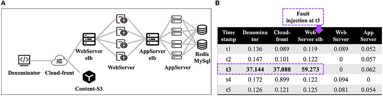
Figure 9. System architecture and example of fault injection. (A) Architecture of microservice system. (B) Response time of services (unit:sm).

The microservice components are interrelated, therefore, the fault injection of a service results in anomaly propagation in the system. We form a group according to the services injected with faults and the services subjected to fault propagation, and the injected node is the root cause node. An example of fault injection is shown in Figure 9B, where a delayed exception is injected into the webserver_elb service at time t3. Based on the system architecture in Figure 9A, the affected services are denominator and cloud-front. We only collect datasets with exceptions, including timestamps, service instances and root cause service with injected faults. We construct two datasets as follows: (i) Dataset A, inject faults into the microservice system every 10 s for a total of 180 times, yielding 152 groups with fault propagation. (ii) Dataset B, inject faults every 30 s for a total of 50 times and obtaining 41 groups with fault propagation. We validate our root cause inference algorithm based on the above dataset, it is worth noting that we do not need to perform content association analysis because the injected faults are all time-delayed anomalies.

We construct association graphs using the relationships between services and analyze groups one by one. For dataset A, our algorithm correctly infers the injected service instance in 144 groups with an accuracy of 94.74%. For dataset B, 40 groups are correctly inferred with an accuracy of 97.56%. There are examples of root cause inference in Figure 10, where the purple node is the inferred root cause. The blue nodes are fault-propagated service instances, the direction of the edge is the propagation direction, and the weight of the edges is the propagation probability and unlabeled edges in light gray with less probability. As shown in Figure 10C, after injecting a time delay fault to the appserver service, the appserver-elb, websever, websever-elb, cloudfront, and denominator services all experience a time delay fault, and the propagation relationship is consistent with the system architecture in Figure 9A.

FIGURE 10

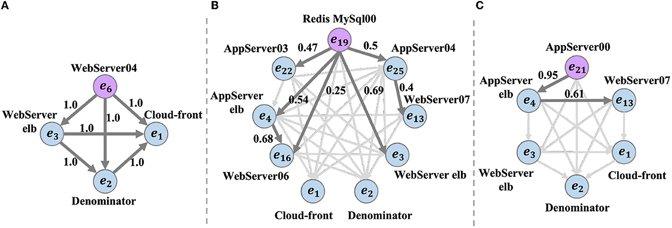
Figure 10. (A–C) Example of root cause inference in microservice system.

5.4. Efficiency analysis

An efficient analysis is needed in real communication networks. Therefore, we counted the number of alarm events occurring in different periods and constructed multiple validation datasets with different alarm events for evaluation. Then we validate the efficiency of two parts of our analysis framework. (i) Offline learning, alarm segmentation is affected by the number of historical alarms, association mining is affected by the number of alarm events, and association reduction is affected by the complexity of the association graph. Figure 11B shows the results of offline learning, which grows linearly with the size of the dataset. (ii) The efficiency of online analysis is also affected by the number of real-time alarms. Figure 11C shows the results of the simulation based on real communication network alarms, illustrating that the efficiency of online analysis also grows linearly with the size of the dataset. In summary, the time complexity of our analysis framework is O(N²). It can deal with massive alarms in large-scale communication networks and effectively reduce the alarm processing time and improve the analysis efficiency.

FIGURE 11

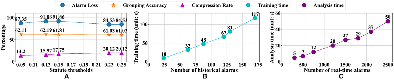
Figure 11. Comparison of statute thresholds and efficiency analysis. (A) Comparison of different statute thresholds. (B) Efficiency analysis of offline learning. (C) Efficiency analysis of online learning.

5.5. Discussion of parameters

5.5.1. Segment threshold

During the segmentation of the historical and real-time alarm sequences, the interval and scenario thresholds are obtained based on the statistical analysis results. We compared different time intervals and scenario thresholds as shown in Figures 12A, B. Due to the limited labeled dataset, the differences in the figures are not obvious, but Figure 12A shows that a smaller time threshold will lose a large number of associations, with the highest rate of alarm loss and the lowest rate of grouping accuracy. While excessive time thresholds obtain a low alarm loss rate but lead to a noisy association. Figure 12B shows that the sequence cannot be segmented with a small scenario threshold, which gets a small rate of alarm loss, but the grouping accuracy is low due to a large number of error associations. However, if the scenario threshold is much larger, it will lose part of the propagation association in the nearby alarm sources, affecting the grouping accuracy. According to the above comparison results, we select the segmentation time threshold of 60 s and the scenario threshold of 0.6 to ensure that the three metrics achieve the best on our dataset.

FIGURE 12

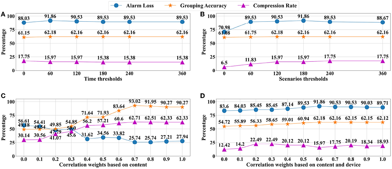
Figure 12. Comparison of different parameters. (A) Comparison of different time thresholds. (B) Comparison of different scenarios thresholds. (C) Comparison of correlation weights based on template e^ind. (D) Comparison of correlation weights based on template e^mix.

5.5.2. Association weight

When constructing the association matrix, we use the association weight parameter α to control the weight of context dependency and alarm content similarity in the association value (Equation 4). To find an appropriate threshold, we compare different weights based on two regular templates as shown in Figures 12C, D. The template e^ind based on alarm titles has a large impact on the parameter change, and α = 0.7 get the best grouping result. The template e^mix based on title and device attributes has little effect on parameter changes, and α = 0.6 get the best grouping result. Therefore, e^mix based on complex attributes has stronger stability, and the grouping accuracy is not easily affected by parameters but will be affected by the label granularity.

5.5.3. Association reduction threshold

The number of invalid associations affects the partition result of the Louvain algorithm, so it is necessary to eliminate the invalid edges with an appropriate reduction threshold β. We compare thresholds of 0.13, 0.15, 0.23, and 0.25 as shown in Figure 11A. When β = 0.23 and β = 0.25, all metrics are stable, but more alarm loss leads to a lower grouping accuracy. When β = 0.09, the number of alarm losses is minimum, but the grouping result is not accurate enough. When β = 0.13 and β = 0.15, a higher grouping accuracy can be obtained. When β = 0.13, fewer alarms are lost, the compression degree of real-time alarms is higher, and obtain the best associations compression result.

6. Related work

The popular alarm analysis and management systems in the industry (BingShow, PagerDuty, BigPanda, Moogsoft) tend to use simple alarm strategies to improve versatility and adapt to diverse application scenarios, such as merging alarms according to their devices or merging adjacent alarms based on a priori topology knowledge. Such systems are effective when applied to regular data, but are less effective in complex data. In addition, these systems usually extract associations based on complete and fine-grained system topological diagrams, but in large-scale systems and complex communication networks with a large number of services and many device components, it is difficult to obtain accurate and stable topology knowledge. At present, the AIOps solutions proposed by enterprises and operators in the real environment are less targeted, and the accuracy is affected by excessive focus on program generality due to the large differences in types of abnormal information in diverse systems. Therefore, there is still room for development in this field.

6.1. Time series segmentation

Traditional methods of time series analysis are mainly implemented based on parameter estimation (Chandola et al., 2009). However, prior knowledge is difficult to obtain for real environments, and methods based on non-parametric estimation are more widely used, such as data-based spatial density distributions (Wu et al., 2014) or deviation distributions (Costa et al., 2019). Another commonly used method is based on the Hawkes Process of self-excited point processes for time series analysis, where the density function is not only time-dependent but also controls the effect of the historical situation on the present through the intensity function (Mei et al., 2017). To obtain more accurate intensity functions, methods based on machine learning and reinforcement learning have also become hot research topics in recent years (Du et al., 2016; Yan et al., 2019). The above methods have certain requirements for data distribution, therefore, methods based on time series statistics have also been widely used in recent years. For example, the methods of setting sliding time windows to divide the series (Li et al., 2015), clustering the time series (Aggarwal et al., 2003; Pham et al., 2009), dividing the time series by temporal features and related attributes. Those methods do not need to consider the distribution of the data and are more suitable for irregularly distributed communication network alarms.

6.2. Alarm association analysis

The aggregation and reduction of alarm events can effectively improve data quality and reduce the cost of locating the root cause of faults (Mansoor et al., 2022). Traditional alarm association analysis methods mainly rely on manual analysis, such as those based on instance inference (Kolodner, 2014), simple models (Chao and Liu, 2004) and a priori rules (Abraham, 1988). The mainstream mining association rule methods are based on the frequent mining algorithm, such as the Apriori algorithm (Shuiyao et al., 2020; Zheng et al., 2020; Zhu, 2020) with FP-Growth algorithm (He et al., 2020; Wang et al., 2020); and methods based on sequential pattern mining algorithm, such as WINEPI algorithm (Lin et al., 2019) with PrefixSpan algorithm (Niyazmand and Izadi, 2019). This type of approach learns rules from data but requires accurate and low-complex event sequences to achieve reliable results. Meanwhile, data-driven approaches based on data mining algorithms, such as the construction of association knowledge using data mining algorithms (Xuewei et al., 2014), association prediction using probabilistic models (Marvasti, 2015), and feature decomposition-based approaches, such as capturing spatiotemporal associations through tensor decomposition (Kimura et al., 2015), have also been used for association analysis. In addition, there are methods based on neural networks for association analysis, such as fault detection models using LSTM neural networks (Liu et al., 2018), capturing spatiotemporal associations of anomalies through deep learning methods (Yuan et al., 2018), and building alarm analysis and prediction frameworks (Zhang and Wang, 2019). In addition, there are approaches to convert alarm analysis to natural language processing problems, such as APE (Chen et al., 2019) is a probabilistic model for association analysis based on Word Embedding. CAR (Lin et al., 2018) ranks alarms based on word embedding to analyze content association. And methods model sequences as n-tuples grammar trees (Hubballi et al., 2011) and compute anomalous inter-sequence associations using machine translation models (Nie et al., 2020). Log2Vec (Meng et al., 2020) is also a log analysis framework that combines word embedding with OOV word processors. There are also alarm reduction methods in cloud systems, such as iPACK (Liu et al., 2023) is an incident-aware method for aggregating duplicate tickets and alerts that considers failure information from both the customer and cloud sides. GRLIA (Chen et al., 2021) is also an incident aggregation framework based on graph representation learning over the cascading graph of cloud failures. The proposed framework learns a representation vector for each unique type of incident in an unsupervised and unified manner that can encode both topological and temporal correlations among incidents.

6.3. Alarm root cause localization

Alarm root cause analysis has become an increasingly important topic of research investigated by many researchers (Alinezhad et al., 2022). Traditional alarm root cause localization methods are mainly based on expert experience to manually label root causes or use supervised learning and semi-supervised learning (Musumeci et al., 2020) to locate root causes. The supervised approaches are less feasible due to the difficulty of obtaining a large amount of labeled alarm data in real environments. In contrast, unsupervised methods are more suitable, such as Granger causal analysis methods (Seth, 2007), based on Granger causality graphs (Liu et al., 2020), and the construction of causal probability graphs based on probabilistic relationships to locate root causes (Marvasti, 2015). In recent years, another hot research defines the root cause location problem as a problem based on fault propagation graphs, such as causal model analysis based on Bayesian network graphs (Wunderlich and Niggemann, 2017), heuristic algorithms based on fault propagation graphs with random wandering (Wang et al., 2018; Weng et al., 2018; Ma et al., 2019), and methods that apply the importance ranking idea of PageRank (Page et al., 1999) algorithm to infer root causes (Treinen and Thurimella, 2007; Zhang et al., 2017). Such methods can quickly infer the effective root cause in fault propagation graphs by optimizing the ranking process to get the key nodes in the causal graph. APGNN (Jiang and Bai, 2023) propose a novel data-driven approach for propagation-based root cause analysis and fault detection, which involves associating alarms and extracting a root-derived graph based on Bayesian Network, constructing alarm propagation graphs (APGs), refining repair orders for actual fault information, and using Graph Neural Network to extract features and learn the mapping from APG to the true fault. ImpactTracer (Xie et al., 2023) builds an impact graph to provide a complete view of fault propagation in microservices and uses a novel backward tracing algorithm that exhaustively traverses the impact graph to identify the root cause node accurately.

7. Conclusion

To address the difficulties in current communication network operation and maintenance, this paper proposes a data-driven and unsupervised alarm analysis framework, which is trained by historical alarms to obtain strongly correlated alarm groups after association reduction and apply to the matching and compression of real-time alarms. The model outputs the compressed groups with inferred root causes. We evaluated the analysis framework based on real communication network alarm data and validated the accuracy of the root cause inference algorithm based on the monitoring data after fault injection in the microservice system. The results show that our method can precisely capture alarm associations. Moreover, it can correctly compress and group more than 91% of alarms, ensuring accurate and reliable analysis results. It also can reduce the number of pending tasks by more than 62%, significantly reducing the burden of operation and maintenance. It further infers root cause alarms with more than 95% accuracy, providing key information for analysis. In future work, we will expand the applicability of our framework, such as analyzing the cross-range propagation and long-term dependence of communication network alarms, optimizing the method of determining the propagation direction among episodic alarms, and reducing the dependence on expert experience in the construction of documents related to alarm content association analysis.

Data availability statement

The data analyzed in this study is subject to the following licenses/restrictions: The experimental data used in this paper comes from real data of enterprises, which involves confidential information about enterprise operations and cannot be disclosed. We will disclose it after declassification. Requests to access these datasets should be directed to chenpf7@mail.sysu.edu.cn.

Author contributions

ML and MY contributed to the conception and design of the study, collected the dataset, and performed the statistical analysis. PC supervised the findings of this work. ML verified the analytical methods and wrote the first draft of the manuscript. All authors contributed to the manuscript revision and approved the submitted version.

Funding

This research was supported by the National Key Research and Development Program of China (No. 2019YFB1804002), the National Natural Science Foundation of China (No. 62272495), the Guangdong Basic and Applied Basic Research Foundation (No. 2023B15150200), and the Fundamental Research Funds for the Central Universities, Sun Yat-sen University (No. 22qntd1004).

Conflict of interest

The authors declare that the research was conducted in the absence of any commercial or financial relationships that could be construed as a potential conflict of interest.

Publisher's note

All claims expressed in this article are solely those of the authors and do not necessarily represent those of their affiliated organizations, or those of the publisher, the editors and the reviewers. Any product that may be evaluated in this article, or claim that may be made by its manufacturer, is not guaranteed or endorsed by the publisher.

References

Abele, L., Anic, M., Gutmann, T., Folmer, J., Kleinsteuber, M., and Vogel-Heuser, B. (2013). Combining knowledge modeling and machine learning for alarm root cause analysis. IFAC Proc. 46, 1843–1848. doi: 10.3182/20130619-3-RU-3018.00057

CrossRef Full Text | Google Scholar

Abraham, A. (1988). “Rule-based expert systems,” in Proceedings of the International Conference on Systems, Man and Cybernetics (IEEE), 610–615.

Google Scholar

Aggarwal, C. C., Han, J., Wang, J., and Yu, P. S. (2003). On clustering massive data streams: a summarization paradigm. SIGMOD Record. 32, 18–25.

Google Scholar

Alinezhad, H. S., Roohi, M. H., and Chen, T. (2022). A review of alarm root cause analysis in process industries: common methods, recent research status and challenges. Chem. Eng. Res. Design. doi: 10.1016/j.cherd.2022.10.041

CrossRef Full Text | Google Scholar

Basha, N., Sheriff, M. Z., Kravaris, C., Nounou, H., and Nounou, M. (2020). Multiclass data classification using fault detection-based techniques. Comp. Chem. Eng. 136, 106786. doi: 10.1016/j.compchemeng.2020.106786

CrossRef Full Text | Google Scholar

Berkhin, P. (2005). A survey on pagerank computing. Int. Math. 2, 73–120. doi: 10.1080/15427951.2005.10129098

CrossRef Full Text | Google Scholar

Bernardo, J. M., and Smith, A. F. (2009). Bayesian Theory, Vol. 405. John Wiley & Sons.

Google Scholar

Bodon, F. (2000). “A fast apriori implementation,” in European Conference on Principles of Data Mining and Knowledge Discovery (Springer), 111–122.

Google Scholar

Borgelt, C. (2005). “An implementation of the FPGrowth algorithm in C++,” in Proceedings of the 1st International Workshop on Open Source Data Mining: Frequent Pattern Mining Implementations (ACM), 1–5.

Google Scholar

Chandola, V., Banerjee, A., and Kumar, V. (2009). Anomaly detection: a survey. ACM Comp. Surv. 41, 1–58. doi: 10.1145/1541880.1541882

CrossRef Full Text | Google Scholar

Chao, C.-S., and Liu, A.-C. (2004). An alarm management framework for automated network fault identification. Comput. Commun. 27, 1341–1353. doi: 10.1016/j.comcom.2004.04.009

CrossRef Full Text | Google Scholar

Chen, H., Chen, P., and Yu, G. (2020). A framework of virtual war room and matrix sketch-based streaming anomaly detection for microservice systems. IEEE Access 8, 43413–43426. doi: 10.1109/ACCESS.2020.2977464

CrossRef Full Text | Google Scholar

Chen, Y., Wang, S., Li, J., Huang, H., and Zhang, Y. (2019). “Entity embedding based anomaly detection for heterogeneous categorical events,” in Proceedings of the 25th ACM SIGKDD International Conference on Knowledge Discovery & Data Mining. p. 2758–2766.

Google Scholar

Chen, Z., Liu, P., Wang, Y., Gu, R., and Huang, X. (2021). Graph-based incident aggregation for large-scale online service systems. IEEE Trans. Serv. Comput. 14, 219–232.

Google Scholar

Coscia, M., Giannotti, F., and Pedreschi, D. (2011). A classification for community discovery methods in complex networks. Stat. Anal. Data Mining 4, 512–546. doi: 10.1002/sam.10133

CrossRef Full Text | Google Scholar

Costa, B. S. J., Bezerra, B. L. D., Lima, R. C. M., Cavalcante-Neto, J., and Lima-Neto, F. B. (2019). Online fault detection based on typicality and eccentricity data analytics. IEEE Trans. Indust. Informat. 6, 3732–3741.

Google Scholar

De Meo, P., Ferrara, E., Fiumara, G., and Provetti, A. (2011). “Generalized Louvain method for community detection in large networks,” in International Conference on Advances in Social Networks Analysis and Mining (IEEE), 32–39.

Google Scholar

Dorgo, G., and Abonyi, J. (2018). Sequence mining based alarm suppression. IEEE Access 6, 15365–15379. doi: 10.1109/ACCESS.2018.2797247

CrossRef Full Text | Google Scholar

Du, N., Zhang, X., Sun, L., and Zhang, J. (2016). “Modeling the intensity function of point process via recurrent neural networks,” in 2016 IEEE International Conference on Data Mining (ICDM) (IEEE), 1095–1100.

Google Scholar

Ester, M., Kriegel, H.-P., Sander, J., and Xu, X. (1996). Density-based spatial clustering of applications with noise. In Int. Conf. Knowl. Discov. Data Mining 6, 240.

PubMed Abstract | Google Scholar

Han, J., Pei, J., Mortazavi-Asl, B., Pinto, H., Chen, Q., Dayal, U., et al. (2001). “Prefixspan: mining sequential patterns efficiently by prefix-projected pattern growth,” in Proceedings of the 17th International Conference on Data Engineering (IEEE), 215–224.

PubMed Abstract | Google Scholar

Hartigan, J. A., and Wong, M. A. (1979). Algorithm as 136: a k-means clustering algorithm. J. R. Stat. Soc. Ser. C 28, 100–108. doi: 10.2307/2346830

CrossRef Full Text | Google Scholar

He, Y. (2020). Research on alarm association mechanism of information system based on fp-growth algorithm. J. Phys. Conf. Ser. 1693, 012082. doi: 10.1088/1742-6596/1693/1/012082

CrossRef Full Text | Google Scholar

Hu, W., Chen, T., and Shah, S. L. (2017). Discovering association rules of mode-dependent alarms from alarm and event logs. IEEE Transact. Cont. Syst. Technol. 26, 971–983. doi: 10.1109/TCST.2017.2695169

CrossRef Full Text | Google Scholar

Hubballi, N., Biswas, S., and Nandi, S. (2011). “Sequencegram: n-gram modeling of system calls for program based anomaly detection,” in 2011 Third International Conference on Communication Systems and Networks (COMSNETS 2011) (IEEE), 1–10.

Google Scholar

Jiang, W., and Bai, Y. (2023). Apgnn: alarm propagation graph neural network for fault detection and alarm root cause analysis. Comp. Netw. 220, 109485. doi: 10.1016/j.comnet.2022.109485

CrossRef Full Text | Google Scholar

Jieba. (2020).Jieba.Available online at: https://github.com/fxsjy/jieba

Google Scholar

Kimura, T., Akagi, S., Arakawa, Y., and Kawahara, Y. (2015). Spatio-temporal factorization of log data for understanding network events. IEEE Trans. Knowl. Data Engg. 27, 2381–2394.

Google Scholar

Kolodner, J. (2014). Case-Based Reasoning. Morgan Kaufmann.

Google Scholar

Ksentini, A., and Pujolle, G. (2006). Evaluation of multicast and unicast routing protocols performance for group communication with QoS constraints in 802.11 mobile ad-hoc networks. Wireless Pers. Commun. 39, 377–396.

Google Scholar

Li, T.-Y., Zhang, Y., and Liu, X. (2015). “Study of alarm pretreatment based on double constraint sliding time window,” in 2015 IEEE International Conference on Cyber Technology in Automation, Control, and Intelligent Systems (CYBER) (IEEE), 1384–1387.

Google Scholar

Li, Y., Chen, Q., Zhang, Y., Xu, H., and Yang, Z. (2018). Word embedding for understanding natural language: a survey. Front. Comput. Sci. 12, 681–696.

Google Scholar

Li, Y., Sun, Y., and Luo, J. (2010). Application of Winepi mining algorithm in IDS. J. Comput. Infm. Syst. 6, 951–958.

Google Scholar

Lin, P., Ye, K., Chen, M., and Xu, C.-Z. (2019). “Dcsa: using density-based clustering and sequential association analysis to predict alarms in telecommunication networks,” in 2019 IEEE 25th International Conference on Parallel and Distributed Systems (ICPADS) (IEEE), 1–8.

Google Scholar

Lin, Y., Chen, Z., Cao, C., Tang, L.-A., Zhang, K., and Li, Z. (2018). Collaborative alerts ranking for anomaly detection. arXiv [Preprint]. arXiv: 1612.07736

Google Scholar

Liu, J., He, S., Chen, Z., Li, L., Kang, Y., Zhang, X., et al. (2023). “Incident-aware duplicate ticket aggregation for cloud systems,” in arXiv [Preprint]. arXiv: 2302.09520

Google Scholar

Liu, Y., Chen, H.-S., Wu, H., Dai, Y., Yao, Y., and Yan, Z. (2020). Simplified granger causality map for data-driven root cause diagnosis of process disturbances. J. Process Control 95, 45–54. doi: 10.1016/j.jprocont.2020.09.006

CrossRef Full Text | Google Scholar

Liu, Y., Li, X., Li, Y., Li, Y., and Li, Y. (2018). “Towards the use of lstm-based neural network for industrial alarm systems,” in 2018 IEEE International Conference on Prognostics and Health Management (ICPHM), 1–6.

Google Scholar

Long, X., Zheng, W., and Chen, C. (2020). Cloud native intelligent operation and maintenance technology. J. Phys. Conf. Ser. 1645, 012028.

Google Scholar

Ma, M., Lin, Z., Wang, W., Zu, J., Liu, H., Li, Z., et al. (2019). “MS-Rank: Multi-metric and self-adaptive root cause diagnosis for microservice applications,” in Proceedings of the 2019 ACM SIGMOD International Conference on Management of Data (ACM), 1741–1758.

Google Scholar

Mansoor, N., Muske, T., Serebrenik, A., and Sharif, B. (2022). “An empirical assessment on merging and repositioning of static analysis alarms,” in 2022 IEEE 22nd International Working Conference on Source Code Analysis and Manipulation (SCAM) (IEEE), 219–229.

Google Scholar

Marvasti, M. (2015). An anomaly event correlation engine: Identifying root causes, bottlenecks, and black swans in IT environments. J. Netw. Comput. Appl. 57, 1–21.

Google Scholar

Mei, H., Eisner, J., Yang, T., Gan, Z., and Wang, F. (2017). The neural hawkes process: A neurally self-modulating multivariate point process. J. Mach. Learn. Res. 18, 6274–6309.

Google Scholar

Meng, W., Liu, Y., Huang, Y., Zhang, S., Zaiter, F., Chen, B., et al. (2020). “A semantic-aware representation framework for online log analysis,” in 2020 29th International Conference on Computer Communications and Networks (ICCCN) (IEEE), 1–7.

Google Scholar

Musumeci, F., Magni, L., Ayoub, O., Rubino, R., Capacchione, M., Rigamonti, G., et al. (2020). Supervised and semi-supervised learning for failure identification in microwave networks. IEEE Transact. Netw. Serv. Manag. 18, 1934–1945. doi: 10.1109/TNSM.2020.3039938

CrossRef Full Text | Google Scholar

Nie, B., Xu, J., Alter, J., Chen, H., and Smirni, E. (2020). “Mining multivariate discrete event sequences for knowledge discovery and anomaly detection,” in 2020 50th Annual IEEE/IFIP International Conference on Dependable Systems and Networks (DSN) (IEEE), 552–563.

Google Scholar

Niwattanakul, S., Singthongchai, J., Naenudorn, E., and Wanapu, S. (2013). “Using of jaccard coefficient for keywords similarity,” in Proceedings of the International Multiconference of Engineers and Computer Scientists, 380–384.

PubMed Abstract | Google Scholar

Niyazmand, T., and Izadi, I. (2019). Pattern mining in alarm flood sequences using a modified prefixspan algorithm. ISA Trans. 90, 287–293. doi: 10.1016/j.isatra.2018.12.050

PubMed Abstract | CrossRef Full Text | Google Scholar

Page, L., Brin, S., Motwani, R., and Winograd, T. (1999). The PageRank citation ranking: Bringing order to the web. Stanford InfoLab. 1, 1–17.

Google Scholar

Paradis, E., Claude, J., and Strimmer, K. (2004). Ape: analyses of phylogenetics and evolution in r language. Bioinformatics 20, 289–290. doi: 10.1093/bioinformatics/btg412

PubMed Abstract | CrossRef Full Text | Google Scholar

Pham, Q.-K., Raschia, G., Mouaddib, N., Saint-Paul, R., and Benatallah, B. (2009). “Time sequence summarization to scale up chronology-dependent applications,” in Proceedings of the 18th ACM Conference on Information and Knowledge Management, 1137–1146.

Google Scholar

Rosvall, M., and Bergstrom, C. T. (2008). Maps of random walks on complex networks reveal community structure. Proc. Nat. Acad. Sci. U. S. A. 105, 1118–1123. doi: 10.1073/pnas.0706851105

PubMed Abstract | CrossRef Full Text | Google Scholar

Seth, A. (2007). Granger causality. Scholarpedia 2, 1667. doi: 10.4249/scholarpedia.1667

CrossRef Full Text | Google Scholar

Shuiyao, C., Lanxin, Q., Weiping, S., and Tao, L. (2020). “Power wireless heterogeneous network management system based on big data technology,” in 2020 IEEE International Conference on Power, Intelligent Computing and Systems (ICPICS) (IEEE), 117–121.

Google Scholar

Tortosa, L., Vicent, J. F., and Yeghikyan, G. (2021). An algorithm for ranking the nodes of multiplex networks with data based on the pagerank concept. Appl. Math. Comput. 392, 125676. doi: 10.1016/j.amc.2020.125676

CrossRef Full Text | Google Scholar

Treinen, J. J., and Thurimella, R. (2007). “Application of the pagerank algorithm to alarm graphs,” in Information and Communications Security: 9th International Conference, ICICS 2007, Zhengzhou, China, December 12-15, 2007. Proceedings 9 (Springer), 480–494.

Google Scholar

Vapnik, V. N. (1999). An overview of statistical learning theory. IEEE Transact. Neural Netw. 10, 988–999. doi: 10.1109/72.788640

PubMed Abstract | CrossRef Full Text | Google Scholar

Wang, P., Xu, J., Ma, M., Lin, W., Pan, D., Wang, Y., et al. (2018). “Cloudranger: root cause identification for cloud native systems,” in 2018 18th IEEE/ACM International Symposium on Cluster, Cloud and Grid Computing (CCGRID) (IEEE), 492–502.

Google Scholar

Wang, K. R., Hu, W., and Chen, T. (2020). “An efficient method to discover association rules of mode-dependent alarms based on the fp-growth algorithm,” in 2020 IEEE Electric Power and Energy Conference (EPEC) (IEEE), 1–5.

Google Scholar

Wen, G., Feng, Z., Wei, H., and Zhang, W. (2015). System optimization strategy of alarm storm. J. Comput. Theoret. Nanosci. 12, 327–334.

Google Scholar

Weng, J., Wang, J. H., Yang, J., and Yang, Y. (2018). Root cause analysis of anomalies of multitier services in public clouds. IEEE/ACM Transact. Netw. 26, 1646–1659. doi: 10.1109/TNET.2018.2843805

CrossRef Full Text | Google Scholar

Wu, K., Zhang, K., Fan, W., Edwards, A., and Philip, S. Y. (2014). “Rs-forest: a rapid density estimator for streaming anomaly detection,” in 2014 IEEE International Conference on Data Mining (IEEE), 600–609.

PubMed Abstract | Google Scholar

Wunderlich, P., and Niggemann, O. (2017). “Structure learning methods for bayesian networks to reduce alarm floods by identifying the root cause,” in 2017 22nd IEEE International Conference on Emerging Technologies and Factory Automation (ETFA) (IEEE), 1–8.

Google Scholar

Xie, R., Yang, J., Li, J., and Wang, L. (2023). “Impacttracer: root cause localization in microservices based on fault propagation modeling,” in 2023 Design, Automation & Test in Europe Conference & Exhibition (DATE) (IEEE), 1–6.

Google Scholar

Xiong, J., and Xiao, W. (2021). Identification of key nodes in abnormal fund trading network based on improved pagerank algorithm. J. Phys. Conf. Ser. 1774, 012001. doi: 10.1088/1742-6596/1774/1/012001

CrossRef Full Text | Google Scholar

Xuewei, F., Dongxia, W., Minhuan, H., and Xiaoxia, S. (2014). “An approach of discovering causal knowledge for alert correlating based on data mining,” in 2014 IEEE 12th International Conference on Dependable, Autonomic and Secure Computing (IEEE), 57–62.

Google Scholar

Yan, Z., Li, W., Liu, X., Li, C., and Liu, Z. (2019). Recent advance in temporal point process: A review from a machine learning perspective. Neurocomputing. 335, 98–113.

Google Scholar

Yu, Y., Si, X., Hu, C., and Zhang, J. (2019). A review of recurrent neural networks: Lstm cells and network architectures. Neural Comput. 31, 1235–1270. doi: 10.1162/neco_a_01199

PubMed Abstract | CrossRef Full Text | Google Scholar

Yuan, Z., Zhou, X., and Yang, T. (2018). “Hetero-convlstm: a deep learning approach to traffic accident prediction on heterogeneous spatio-temporal data,” in Proceedings of the 24th ACM SIGKDD International Conference on Knowledge Discovery & Data Mining, 984–992.

Google Scholar

Zhang, M., Li, X., Zhang, L., and Khurshid, S. (2017). “Boosting spectrum-based fault localization using pagerank,” in Proceedings of the 26th ACM SIGSOFT International Symposium on Software Testing and analysis, 261–272.

Google Scholar

Zhang, M., and Wang, D. (2019). “Machine learning based alarm analysis and failure forecast in optical networks,” in 2019 24th OptoElectronics and Communications Conference (OECC) and 2019 International Conference on Photonics in Switching and Computing (PSC) (IEEE), 1–3.

Google Scholar

Zhao, N., Chen, J., Peng, X., Wang, H., Wu, X., Zhang, Y., et al. (2020). “Understanding and handling alert storm for online service systems,” in 2020 IEEE/ACM 42nd International Conference on Software Engineering: Software Engineering in Practice (ICSE-SEIP) (IEEE), 162–171.

Google Scholar

Zheng, Q., Li, Y., and Cao, J. (2020). Application of data mining technology in alarm analysis of communication network. Comput. Commun. 163, 84–90. doi: 10.1016/j.comcom.2020.08.012

CrossRef Full Text | Google Scholar

Zhu, L. (2020). Implementation of web log mining device under apriori algorithm improvement and confidence formula optimization. Int. J. Inf. Technol. Web Eng. 15, 53–71. doi: 10.4018/IJITWE.2020100104

CrossRef Full Text | Google Scholar

Zhu, X., Ghahramani, Z., and Lafferty, J. (2003). “Learning from labeled and unlabeled data with label propagation,” in Proceedings of the 20th International Conference on Machine Learning (ICML-03) (AAAI Press), 912–919.

Google Scholar