Good continuation in 3D: the neurogeometry of stereo vision

Classical good continuation for image curves is based on 2D position and orientation. It is supported by the columnar organization of cortex, by psychophysical experiments, and by rich models of (differential) geometry. Here, we extend good continuation to stereo by introducing a neurogeometric model to abstract cortical organization. Our model clarifies which aspects of the projected scene geometry are relevant to neural connections. The model utilizes parameterizations that integrate spatial and orientation disparities, and provides insight into the psychophysics of stereo by yielding a well-defined 3D association field. In sum, the model illustrates how good continuation in the (3D) world generalizes good continuation in the (2D) plane.

1 Introduction

Binocular vision is the ability of the visual system to provide information about the three-dimensional environment starting from two-dimensional retinal images. Disparities are among the main cues for depth perception and stereo vision but, in order to extract them, the brain needs to determine which features coming from the right eye correspond to those from the left eye, and which do not. This generates a coupling problem, which is usually referred to as the stereo correspondence problem. Viewed in the large, stereo correspondence must be consistent with stereo perception more generally, and knowing the relevant features is key for both issues. In this paper we develop an approach to stereo based on the functional organization of the visual cortex, and we identify the geometric features extracted by the binocular cells. This model will be able to extend the notion of good continuation for planar curves to that for 3D spatial curves. A simple example demonstrates their application in computing stereo correspondence.

Good continuation in the plane (retinotopic coordinates) is one of the foundational principles of Gestalt perceptual organization. It enjoys an extensive history (Wagemans et al., 2012). It is supported by psychophysical investigations (e.g., Field et al., 1993; Geisler et al., 2001; Elder and Goldberg, 2002; Hess et al., 2003; Lawlor and Zucker, 2013), which reveal connections to contour statistics; it is supported by physiology (orientation selectivity), which reveals the role for long-range horizontal connections (Bosking et al., 1997); and it is supported by computational modeling (Ben-Shahar and Zucker, 2004; Sarti et al., 2007), which reveals a key role for geometry. The notion of orientation underlies all three of these aspects: neurons in visual cortex are selective for orientations, pairs of dots in grouping experiments indicate an orientation, and edge elements in natural images are oriented and related to image statistics. Orientation in space involves two angles, which we shall exploit. Nevertheless, good continuation in depth is much less well-developed than good continuation in the plane, despite having comparable historical origins. (Koffka, 1963, p. 161-162):

...a perspective drawing, even when viewed monocularly, does not give the same vivid impression of depth as the same drawing if viewed through a stereoscope with binocular parallax... for in the stereoscope the tri-dimensional force of the parallax co-operates with the other tri-dimensional forces of organization; instead of conflict between forces, stereoscopic vision introduces mutual reinforcement.

Our specific goal in this paper is to develop a neurogeometrical model of stereo vision, based on the functionality of binocular cells. The main application will be a good continuation model in three dimensions that is analogous to the models of contour organization in two dimensions. We will develop ad hoc mathematical instruments, supported by a number of neural and psychophysical investigations (Malach et al., 1993; Uttal, 2013; Deas and Wilcox, 2014, 2015; Khuu et al., 2016; Scholl et al., 2022).

Although only one dimension higher than contours in the plane, contours extending in depth raise subtle new issues; this is why a geometric model can be instructive. First among the issues is the choice of coordinates which, of course, requires a mathematical framework for specifying them. In the plane, position and orientation are natural; smoothness is captured by curvature or the relationship between nearby orientations along a contour. For stereo, there is monocular structure in the left eye and in the right. Spatial disparity is a standard variable relating them, and it is well-known that primate visual systems represent this variable directly (Poggio, 1995). Spatial disparity is clearly a potential coordinate. However, other physiological aspects are less clear. The columnar architecture so powerful for contour organization in the plane is not only monocular: the presence of columns for spatial disparity of binocular cells has been experimentally described in V2 (Ts'o et al., 2009). However, orientation disparity does not seem to be coded in the cortex (see next section). Nevertheless, orientation-selective cells provide the input for stereo so, at a minimum, both position disparity and orientation – one orientation for the right eye and (possibly) another for the left – should be involved. While it is traditional to assume only “like” orientations are matched (Hubel and Wiesel, 1962; Nelson et al., 1977; Marr and Poggio, 1979; Bridge and Cumming, 2001; Chang et al., 2020), our sensitivity to orientation disparity questions this, making orientation disparity another putative variable. We shall show that orientations do play a deep role in stereo, but that it is not necessarily efficient to represent them as a disparity. Furthermore, there is a debate in stereo psychophysics about orientation: since its physiological realization could be confounded with disparity gradients (Mitchison and McKee, 1990; Cagenello and Rogers, 1993), orientation may be redundant. This is not the case, since it is the orientation of the “gradient” that matters. Thus we provide a representation of the geometry of spatial disparity and orientation in support of using good continuation in a manner that both incorporates the biological “givens” and provides a rigorous foundation for the correspondence problem. As has been the case with curve organization, we further believe that our modeling will illuminate the underlying functional architecture for stereo.

Hubel and Wiesel reported disparity-tuned neurons in early, classic work (Hubel and Wiesel, 1970). They observed that single units could be driven from both eyes and that it was possible to plot separate receptive fields (RF) for each eye. We emphasize that these monocular receptive fields are tuned to orientation (Cumming and DeAngelis, 2001; Parker et al., 2016), and a review of neural models can be found in Read (2015).

The classical model for expressing the left/right-eye receptive field combination is the binocular energy model (BEM), first introduced in Anzai et al. (1999b). It encodes disparities through the receptive profiles of simple cells, raising the possibility of both position and phase disparities (Jaeger and Ranu, 2015). However, Read and Cumming (2007), building upon (Anzai et al., 1999a), showed that phase disparity neurons tend to be strongly activated by false correspondence pairs. Other approaches are based on the statistics of natural images (Burge and Geisler, 2014; Jaini and Burge, 2017; Burge, 2020) utilized in an optimal fashion; these lead to more refined receptive field models. Nevertheless, the orientation differences between the two eyes (Nelson et al., 1977), or orientation disparity, should not be neglected. Although there were attempts to incorporate it (Bridge et al., 2001) in energy models, they are limited. The geometrical model we will present incorporates orientation differences directly.

Many other mathematical models for stereo vision based on neural models have been developed. Some claim (e.g., Marr and Poggio, 1979) that orientations should match between the two eyes, although small differences are allowed. This, of course, assumes the structure is frontal-parallel. Subsequently, Jones and Malik (1991) used a set of linear filters tuned to different orientations (and scales) but their algorithm was not built on a neurophysiological basis. Alibhai and Zucker (2000), Li and Zucker (2003), and Zucker (2014) built a more biologically-inspired model that addressed the connections between neurons. Their differential-geometry model employed position, orientations and curvatures in 2D retinal planes, modeling binocular neurons with orientations given by tangent vectors of Frenet geometry. Our results here are related, although the geometry is deeper (We develop this below.). A more recent work, based on differential and Riemannian geometry, is developed in Neilson et al. (2018). Before specifying these results, however, we introduce the specific type of geometry that we shall be using. It follows directly from the columnar organization often seen in predators and primates.

1.1 Columnar architectures and sub-Riemannian geometry

We propose a sub-Riemannian model for the cortical-inspired geometry underlying stereo vision based on the encoding of positional disparities and orientation differences in the information coming from the two eyes. We build on neuromathematical models, starting from the work of Koenderink and van Doorn (1987) and Hoffman (1989), with particular emphasis on the neurogeometry of monocular simple cells (Petitot and Tondut, 1999; Citti and Sarti, 2006; Sarti et al., 2007; Petitot, 2008; Sanguinetti et al., 2010; Sarti and Citti, 2015; Baspinar et al., 2020).

To motivate our mathematical approach, it is instructive to build on an abstraction of visual cortex. We start with monocular information, segregated into ocular dominance bands (LeVay et al., 1975) in layer 4; these neurons have processes that extend into the superficial layers. We cartoon this in Figure 1, which shows an array of orientation hypercolumns arranged over retinotopic position. It is colored by dominant eye inputs; the binocularly-driven cells tend to be closer to the ocular dominance boundaries, while the monocular cells are toward the centers. A zoom emphasizes the orientation distribution along a few of the columns near each position; horizontal connections (not shown) effect the interactions between these units. This raises the basic question in this paper: what is the nature of the interaction among groups of cells representing different orientations at nearby positions and innervated by inputs from the left and right eyes? The physiology suggests (Figure 1C) the answer lies in the interactions among both monocular and binocular cells; our model specifies this interaction, starting from the monocular ones and building analogously into a columnar organization.

Figure 1

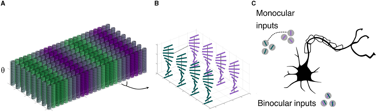
Figure 1. Cartoon of visual cortex, V1, superficial layers. (A) Macroscopic organization: A number of (abstracted) orientation hypercolumns, colored by left-eye (green)/right-eye (purple) dominant inputs. The color grading emphasizes that at the center of the ocular dominance bands the cells are strongly monocular, while at the boundaries they become binocularly-driven. (B) A zoom in to a few orientation columns showing left and right monocular cells at the border of ocular dominance bands. Cells in these nearby columns will provide the anatomical substrate for our model. (C) More recent work shows that both monocular and binocular inputs matter to these cells (redrawn from Scholl et al., 2022, using data from ferret). This more advanced wiring suggests the connection structures in our model.

1.2 Informal setup and overview

Since much of the paper is technical, we here specify, informally, the main ingredients of the model and the results. We first list several of the key points, then illustrate them directly.

• Stereo geometry enjoys a mathematical structure that is a formal extension of plane curve geometry. In the plane, points belonging to a curve are described by an orientation at a position, and these are naturally represented as elements (orientation, position) of columns. In our model, these become abstract fibers. The collection of fibers across position is a fiber bundle. Elements of the (monocular) fiber can be thought of as neurons.

• Our geometrical model is based on tangents and curvatures. Tangents naturally relate to orientation selectivity, and are commonly identified with “edge” elements in the world. We shall occasionally invoke this relationship, for intuition and convenience, but some caution is required. While edge elements comprising, e.g., a smooth bounding contour are tangents, the converse is not necessarily true (e.g., elongated attached highlights or hair textures). Instead, our model should be viewed as specifying the constraints relevant to understanding neural circuitry; see Section 1.3.

• To elaborate the previous point: the tangents in our model need not be edges in the world; they are neural responses. The constraints in our model can be used to determine whether these responses should be considered as “edges.” This is why the model is built from the geometry of idealized space curves: to support such inferences.

• For stereo, we shall need fibers that are a “product” of the left and right-eye monocular columns. This is the reason why we choose position, positional disparity and orientations from the left and right eyes respectively, as the natural variables that describe the stereo fiber over each position. We stress that these fibers are not necessarily explicit in the cortical architecture.

• Curvature provides a kind of “glue” to enable transitions from points on fibers to nearby points on nearby fibers. These transitions specify “integral curves” through the stereo fiber bundle.

• The integral curve viewpoint provides a direction of information flow (information diffuses through the bundle) thereby suggesting underlying circuits.

• The integral curves formalize association field models. Their parameters describe the spray of curves that is well in accordance with 3D curves as studied in psychophysical experiments in Hess and Field (1995), Hess et al. (1997), and Khuu et al. (2016).

• Our formal theory addresses several conjectures in the literature. The first is the identity hypothesis (Kellman et al., 2005a,b) and the organization of units for curve interpolation (cf. Anderson et al., 2002); we show how tangents are natural “units” and how they can be organized. The second concerns the nature of the organization (Li and Zucker, 2006), where we resolve a conjecture regarding the interpolating object (see Proposition 3.2 below).

• Our formal theory provides a new framework for specifying the correspondence problem, by illustrating how good continuation in the 3-D world generalizes good continuation in the 2-D plane. This is the point where consistent binocular-binocular interactions are most important.

• Our formal theory has direct implications for understanding torsional eye movements. It suggests, in particular, that the rotational component is not simply a consequence of development, but that it helps to undo inappropriate orientation disparity changes induced by eye movements. This role for Listing's Law will be treated in a companion paper (in preparation); see also the excellent paper (Schreiber et al., 2008).

We now illustrate these ideas (Figure 2). Consider a three-dimensional stimulus as a space curve γ:ℝ → ℝ³, with a unit-length tangent at the point of fixation. Since the tangent is the derivative of a curve, the binocular cells naturally encode the unitary tangent direction $\dot{\gamma }$ to the spatial 3D stimulus γ. This space tangent projects to a tangent orientation in the left eye¹, and perhaps the same or a different orientation in the right eye. A nearby space tangent projects to another pair of monocular tangents, illustrated as activity in neighboring columns. Note how connections between the binocular neurons support consistency along the space curve. It is this consistency relationship that we capture with our model of the stereo association field.

Figure 2

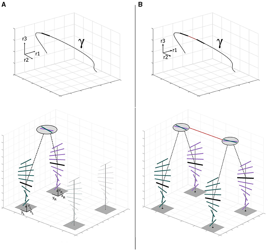
Figure 2. (A) Stereo projection of the highlighted tangent vector to the stimulus γ ∈ ℝ³ in the left-eye innervated and right-eye innervated monocular orientation columns (Each short line denotes a neuron by its orientation preference.). Joint activity across the eyes, which denotes the space tangent, is illustrated by the binocular neuron (circle). Note the two similar but distinct monocular orientations. Connections from the actively stimulated monocular neurons to the binocular neuron are shown as dashed lines. (B) Stereo projection of a consecutive pair of tangents to the stimulus γ ∈ ℝ³ in the left and right retinal columns. Each space tangent projects to a different pair of monocular columns because of the spatial disparity. Consistency in the responses of these four columns corresponds to consistency between the space tangents attached to nearby positions along γ. This consistency is realized through the binocular neural connection (solid line).

Since space curves live in 3D, two angles are required to specify its space tangent at a point. In other words, monocular tangent angles span a circle in the plane; space tangent angles span a 2-sphere in 3D. In terms of the projections into the left-eye and the right-eye, the space tangent can be described by the parameters n = (θ, φ) of 𝕊² (Figure 3A). Thus, we can suitably describe the space of stereo cells – the full set of space tangents at any position in the 3D world – as the manifold of positions and orientations ℝ³ ⋊ 𝕊². Moving from one position in space to another, and changing the tangent orientation to the one at the new position, amounts to what is called a group action on the appropriate manifold. We informally introduce these notions in the next subsection; a more extensive introduction to these ideas is in Appendix A (Supplementary material).

Figure 3

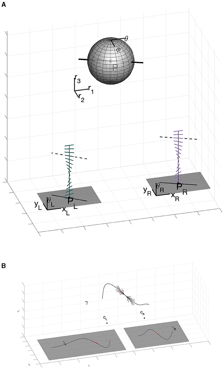
Figure 3. (A) The full geometry of stereo. Note how the stereo correspondence problem allows to establish the relationship between the 3D tangent point (P, θ, ϕ) and the projections p_L and p_R, the disparity and the orientations θ_L and θ_R. (B) Main result of the paper. The three-dimensional space curve γ is enveloped by the 3D association field centered at a point. Formally, this association field is a fan of integral curves in the sub-Riemmanian geometry computed entirely within the columnar architecture (It is specifically described by Equation (36) with varying c₁ and c₂ in ℝ, but that will take some work to develop.).

1.2.1 Sub-Riemannian geometry

We live in a 3D world in which distances are familiar; that is, a space of points with a Euclidean distance function defined between any pair of them. Apart from practical considerations we can move in any direction we would like. Cars, however, have much more restricted movement capabilities. They can move forward or backward, but not sideways. To move in a different direction, cars must turn their wheels. Here is the basic analogy: in cortical space information can move to a new retinotopic position in a tangent direction, or it can move up or down a column (orientation fiber) to change direction. Moving in this fashion, from an orientation at a position to another orientation at a nearby position, is clearly more limited than arbitrary movements in Euclidean space. Euclidean geometry, as above, is an example of a Riemannian geometry; the limitations involved in moving through a cortical columnar space specify a sub-Riemannian geometry (Citti and Sarti, 2014; Citti et al., 2015; Sarti et al., 2019). Just as cars can move along roads that are mostly smooth, excitatory neurons mainly connect to similarly “like” (in orientation) excitatory neurons. This chain of neurons indicates a path through sub-Riemannian space (Agrachev et al., 2019); the fan of such paths is the cortical connectivity which can be considered the neural correlate of association fields. Again, for more information please consult Appendix A (Supplementary material).

Moving now out to the world, we must be able to move between all points. Repeating the above metaphor more technically, we equip ℝ³ ⋊ 𝕊² with a group action of the three-dimensional Euclidean group of rigid motions SE(3). Notice, importantly, that this group is now acting on the product space of positions and orientations. A bit more is required, though, since the geometry of stereo vision is not solved only with these punctual and directional arguments. As we showed in Figure 2 there is the need to take into account the relationships between nearby tangents; in geometric language this involves a suitable type of connections. It is therefore natural to look at integral curves of the sub-Riemannian structure, which encode in their coefficients the fundamental concept of 3D curvature and torsion. An example of this is shown in Figure 3B. Notice how the 3D association field envelopes a space curve, in the same way that a 2D association field envelopes a planar curve. This figure illustrates, in a basic way, the fundamental result in this paper.

1.3 On the neuro-geometric approach

There are many different ways to approach mathematical modeling in vision. One could, for example, ask what is the best an ideal observer could do for the stereo problem working directly on image data (Burge and Geisler, 2014; Burge, 2020). This requires specifying the task, e.g., disparity at a point; a database of images on which the estimation is to be carried out; and a specification of the output. The approach is fundamentally statistical, and has been successful at predicting discrimination thresholds and optimal receptive field designs for patches of natural images. We seek to go the next step – to specify the relationship between receptive fields; i.e., between neurons. Note that the complexity multiplies enormously. At the behavioral level this raises the question of grouping, or determining the combinations of disparities, or Gabor patch samples, that belong together. The complexity arises because this must be evaluated over all possible arrangements of patches, be they along curves, or surfaces, or combinations thereof. In effect, the output specification is pushed toward co-occurrence phenomena, and these toward neural connections.

Our working hypothesis is that there is a deep functional relationship between structure in the brain and structure in the world, and that geometry is the right language with which to capture this relationship, especially as regards connectivity between neurons and their functionality. The neuro-geometric approach is precisely this; an attempt to capture how the structure of cortical connectivity (and other functional properties) are reflected in the phenomena of visual perception.

At first blush this might seem completely unrelated to the statistics of natural images, and how these could be informative of neural connections, but we believe that there is a fundamental relationship. Consider, to start, the distribution of oriented edge elements in a small patch. Pairwise edge statistics are well-studied (August and Zucker, 2000; Geisler et al., 2001; Elder and Goldberg, 2002; Sanguinetti et al., 2010), and indicate how orientation changes are distributed over (spatially) nearby edge elements. Co-linear and co-circular patterns emerge from these studies, as well as in third-order statistics of edges (Lawlor and Zucker, 2013). Interestingly, in Singh and Fulvio (2007) and Geisler and Perry (2009) deviation from co-circular behavior emerges.² In particular, Geisler and Perry (2009) proposes a parabolic model to explain these statistical evidences, that is consistent with previous results if we consider a composition of the joint action of cocircularity and parallelism cues (as found to factor for example in Elder and Goldberg, 2002). To elaborate, it begins by following either a co-circular or linear term, followed by the composition with another circular or linear term. The outcome of this process is described as a spline-like behavior that can approximate a parabola. In Sanguinetti et al. (2010), it has been shown that the histogram of the co-occurrence of edges in a natural image provides the same probability kernel we could find with geometric analysis instruments. As a result, statistical measurements are integrated into the geometric approach.

The geometric analysis that we shall use is continuous mathematics, and is essentially differential (Tu, 2011). This has important implications. First, the relationships that matter are those over small neighborhoods, not over “long” distances. Thus at a point there is an orientation (tangent) and a curvature. These barely change as one moves a tiny distance from the point. Thus we are not considering (in this paper) what happens behind (relatively) large occluders, when longer distances devoid of intermediate structure separate structure (Singh and Fulvio, 2005; Fulvio et al., 2008). Such problems are important but are outside the scope of this paper. Second, because the mathematics is continuous, we shall not consider sampling issues (Warren et al., 2002). To the extent that it matters, we shall assume discrete entities are sufficiently densely distributed that they function as if they were continuous (Zucker and Davis, 1988). In this sense our analysis is restricted to early vision. It does not necessarily account for the full range of cognitive tasks, which may well invoke higher-order computations over longer distances and even richer abstractions.

It has been observed that edge statistics for curves in the world depart from co-circularity. To quote (Geisler and Perry, 2009): “Except for a direction of zero, where the orientation difference is consistent with a collinear relationship, the highest-likelihood orientation differences are less than those predicted by a co-circular relationship.” We believe this has to do with the notion of curvature used: whether it is purely local, or an estimate over distance. In summary of the geometric approach, we explain this as follows. Our constraints can be used in two rather different ways. First, from a computational perspective, one can “integrate” the local constraints into more global objects. This is the approach used in the example section of this paper, and could give rise to an “average” curvature over some distance. The second approach is more distributed, and may be closer to a neurobiological implementation (Ben-Shahar and Zucker, 2004). In this second approach (not developed in this paper, but see Li and Zucker (2006) and Figure 6), the local computations overlap to enforce consistency (The scale of such computations would be a small factor larger than that indicated in Figure 2B). This scale corresponds to the extent of biological “long range horizontal connections” but is smaller than many of the occluders used in psychophysical experiments. In other words, to emphasize this distinction, in the former case the use of integral curves may be closer to the parabolic relations observed in scene statistics (Geisler and Perry, 2009).³ Our use of the term “co-circularity” is in the latter sense.

1.4 Overview of paper

The paper is organized as follows: in Section 2, we describe the geometrical and neuro-mathematical background underlying the problem of stereo vision. In particular, we review the standard stereo triangulation technique to relate the coordinate system of one retina with the other, and put them together in order to reconstruct the three-dimensional space. Then, we briefly review the classical neurogeometry of monocular simple cells selective for orientation and the underlying connections. The generalization of approximate co-circularity for stereo is also introduced. In Section 3, starting from binocular receptive profiles, we introduce the neuro-mathematical model for binocular cells. First we present the cortical fiber bundle of binocular cells. It follows the differential interpretation of the binocular profiles in terms of the neurogeometry of the simple cells, and we show how this is well in accordance with the results of the stereo triangulation. Then, we give a mathematical definition of the manifold ℝ³ ⋊ 𝕊² with the sub-Riemannian structure. Finally, we study the integral curves and the suitable change of variables that allow us to switch our analysis from cortical to external space. In Section 4 we proceed to the validation of our geometry with respect to psychophysical experiments. We combine information about the psychophysics of 3D perception and formal conjectures; it is here that we formulate a 3D association field analogous to the 2D association field. At the end, we show an example of a representation of a stimulus (from image planes to the full 3D and orientation geometry) and how our integral curves properly connect corresponding points. This illustrates the use of our model as a basis for solving the correspondence problem.⁴

2 Stereo vision and neuro-mathematical background

2.1 Stereo geometry

In this subsection, we briefly recall the geometrical configuration underlying 3D vision, to define the variables that we use in the rest of the paper, mainly referring to (Faugeras, 1993, Ch. 6). For a complete historical background see Howard (2012); Howard and Rogers (1995).

2.1.1 Stereo variables

We consider the global reference system (O, i, j, k) in ℝ³, with O = (0, 0, 0), and coordinates (r₁, r₂, r₃). We introduce the optical centers C_L = (−c, 0, 0) and C_R = (c, 0, 0), with c real positive element, and we define two reference systems: (C_L, i_L, j_L), (C_R, i_R, j_R), the reference systems of the retinal planes ${\mathcal{R}}_L$ and ${\mathcal{R}}_R$ with coordinates respectively (x_L, y), (x_R, y). In the global system we suppose the retinal planes to be parallel and to have equation r₃ = f, with f denoting the focal length. This geometrical set-up is shown in Figure 4.

Figure 4

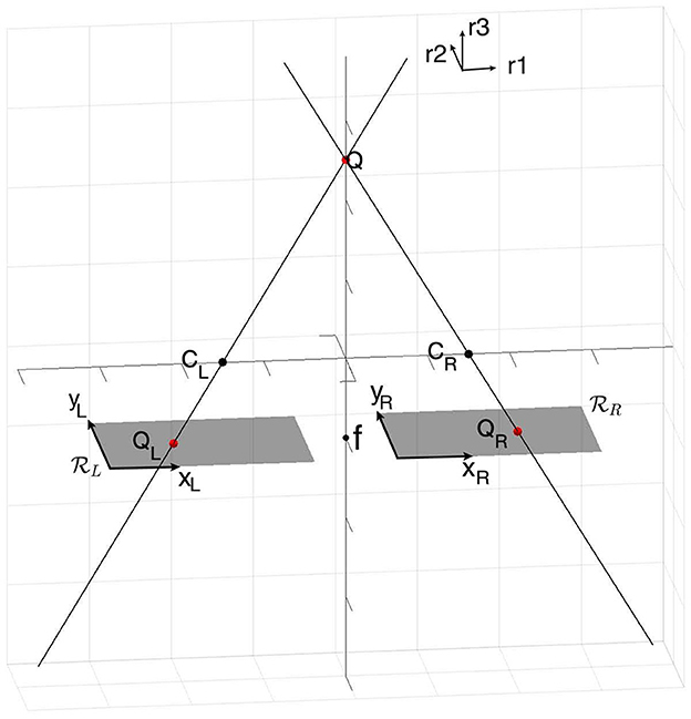
Figure 4. Reconstruction of the 3D space point Q through points Q_L the retinal plane ${\mathcal{R}}_L$ and Q_R in ${\mathcal{R}}_R$.

Remark 2.1. If we know the coordinate of a point $Q={(r_1,r_2,r_3)}^T$ in ℝ³, then it is easy to project it in the two planes via perspective projection, having c the coordinate of the optical centers and f focal length. This computation defines two projective maps Π_L and Π_R, respectively, for the left and right retinal planes:

$\begin{array}{ll}\begin{array}{cccccccc}{\Pi }_L:& {ℝ}^3& \to & {ℝ}^2& {\Pi }_R:& {ℝ}^3& \to & {ℝ}^2\\ \left(\begin{array}{c}{r}_1\\ r_2\\ r_3\end{array}\right)& \mapsto & \left(\begin{array}{c}\frac{f(r_1+c)}{r_3}\\ \frac{f{r}_2}{r_3}\end{array}\right),& & \left(\begin{array}{c}{r}_1\\ r_2\\ r_3\end{array}\right)& \mapsto & \left(\begin{array}{c}\frac{f(r_1-c)}{r_3}\\ \frac{f{r}_2}{r_3}\end{array}\right).\end{array}& (1)\end{array}$

Proof. A point on the left retinal plane of local coordinates ${(x_L,y)}^T$ has global coordinates $Q_L={(-c+x_L,y,f)}^T$, and it corresponds to a point $Q={(r_1,r_2,r_3)}^T$ in the Euclidean ℝ³ such that C_L, Q_L and Q are aligned. This means that the vectors $Q_L-C_L={(x_L,y,f)}^T$ and $Q-C_L={(r_1+c,r_2,r_3)}^T$ are parallel, obtaining the following relationships:

$\begin{array}{ll}{x}_L=f\frac{r_1+c}{r_3},y=f\frac{r_2}{r_3}.& (2)\end{array}$

Analogously, considering Q_R and C_R, we get:

$\begin{array}{ll}{x}_R=f\frac{r_1-c}{r_3},y=f\frac{r_2}{r_3}.& (3)\end{array}$

     □

In a standard way, the horizontal disparity is defined as the differences between retinal coordinates

$\begin{array}{ll}d:=\frac{x_L-x_R}{2},& (4)\end{array}$

up to a scalar factor. Moreover, it is also possible to define the coordinate x as the average of the two retinal coordinates $x:=\frac{x_L+x_R}{2}$, leading to the following change of variables:

$\begin{array}{ll}\{\begin{array}{c}x=\frac{f{r}_1}{r_3}\\ y=\frac{f{r}_2}{r_3}\\ d=\frac{fc}{r_3}\end{array}\leftrightarrow \{\begin{array}{c}{r}_1=\frac{xc}{d}\\ r_2=\frac{yc}{d}\\ r_3=\frac{fc}{d}\end{array},& (5)\end{array}$

where the set of coordinates (x, y, d) is known as cyclopean coordinates (Julesz, 1971).

2.1.2 Tangent estimation

Corresponding points in the retinal planes allow to project back into ℝ³. An analogous reasoning can be done for the tangent structure: if we have tangent vectors of corresponding curves in the retinal planes, it is possible to project back and recover an estimate of the 3D tangent vector. Let us recall here this result; a detailed explanation can be found in Faugeras (1993).

Remark 2.2. Let γ_L and γ_R be corresponding left and right retinal curves; i.e., perspective projections of a curve γ ∈ ℝ³ through optical centers C_L and C_R with focal length f. Knowing the left and right retinal tangent structures, it is possible to recover the direction of the tangent vector $\dot{\gamma }$.

Proof. Starting from a curve γ ∈ ℝ³, we project it in the two retinal planes obtaining γ_L = Π_L(γ) and γ_R = Π_R(γ) from Equation (1). The retinal tangent vectors are obtained through the Jacobian matrix⁵ of the left and right retinal projections ${\dot{\gamma }}_{L,R}(t)={(J_{{\Pi }_{L,R}})}_{\gamma (t)}\dot{\gamma }(t)$:

$\begin{array}{ll}{\dot{\gamma }}_R(t)=\left(\begin{array}{c}\frac{f({\gamma }_3{\dot{\gamma }}_1+(c-{\gamma }_1){\dot{\gamma }}_3)}{{\gamma }_3{(t)}^2}\\ \frac{f({\gamma }_3{\dot{\gamma }}_2-{\gamma }_2{\dot{\gamma }}_3)}{{\gamma }_3^2}\end{array}\right),{\dot{\gamma }}_L(t)=\left(\begin{array}{c}\frac{f({\gamma }_3{\dot{\gamma }}_1-(c+{\gamma }_1){\dot{\gamma }}_3)}{{\gamma }_3{(t)}^2}\\ \frac{f({\gamma }_3{\dot{\gamma }}_2-{\gamma }_2{\dot{\gamma }}_3)}{{\gamma }_3^2}\end{array}\right).& (6)\end{array}$

Extending the tangent vectors and the points into ℝ³, we get ${\tilde{t}}_L={({\dot{\gamma }}_{L1},{\dot{\gamma }}_{L2},0)}^T$, and ${\tilde{m}}_L={({\gamma }_{L1}-c,{\gamma }_{L2},f)}^T$, and $U_{t_L}={(P_L)}^{-1}{\tilde{m}}_L\times (P_L^{-1}){\tilde{t}}_L$, with the projection matrix $P_L=\left(\begin{array}{ccc}1& 0& -c/f\\ 0& 1& 0\\ 0& 0& 1\end{array}\right)$. The same reasoning holds for the right structure, with projection matrix $P_R=\left(\begin{array}{ccc}1& 0& c/f\\ 0& 1& 0\\ 0& 0& 1\end{array}\right)$.

Then U_tR × U_tL is a vector parallel to the tangent vector $\dot{\gamma }$:

$\begin{array}{ll}\begin{array}{l}{U}_{t_R}\times U_{t_L}={\left(\begin{array}{l}{\displaystyle \underset{\lambda (t)}{{\displaystyle \underbrace{\frac{f^{4}2c({\dot{\gamma }}_2{\gamma }_3-{\dot{\gamma }}_3{\gamma }_2)}{{\gamma }_3^4}}}}}{\dot{\gamma }}_1,\\ \frac{f^{4}2c({\dot{\gamma }}_2{\gamma }_3-{\dot{\gamma }}_3{\gamma }_2)}{{\gamma }_3^4}{\dot{\gamma }}_2,\frac{f^{4}2c({\dot{\gamma }}_2{\gamma }_3-{\dot{\gamma }}_3{\gamma }_2)}{{\gamma }_3^4}{\dot{\gamma }}_3\end{array}\right)}^T\\ =\lambda (t){({\dot{\gamma }}_1(t),{\dot{\gamma }}_2(t),{\dot{\gamma }}_3(t))}^T\\ =\lambda (t)\dot{\gamma }(t).\end{array}& (7)\end{array}$

     □

Although this section has been based on the geometry of space curves and their projections, we observe that related geometric approaches have been developed for planar patches and surfaces; see, e.g., Li and Zucker, 2008; Oluk et al., 2022 and references therein.

2.2 Elements of neurogeometry

We now provide background on the geometric modeling of the monocular system, and good continuation in the plane. Our goal is to illustrate the role of sub-Riemannian geometry in the monocular system, which will serve as the basis for generalization to the stereo system.

2.2.1 Classical neurogeometry of simple cells

We model the activation map of a cortical neuron's receptive field (RF) by its receptive profile (RP) φ. A classical example is the receptive profiles of simple cells in V1, centered at position (x, y) and orientation θ, modeled (e.g., in Daugman, 1985; Jones and Palmer, 1987; Barbieri et al., 2014b) as a bank of Gabor filters φ_{{x, y, θ}}. RPs are mathematical models of receptive fields; they are operators which act on a visual stimulus.

Formally, it is possible to abstract the primary visual cortex as ℝ² × 𝕊¹, or position-orientation space, thereby naturally encoding the Hubel/Wiesel hypercolumnar structure (Hubel and Wiesel, 1962). An example of this structure is displayed in Figure 5D from Ben-Shahar and Zucker (2004).

Figure 5

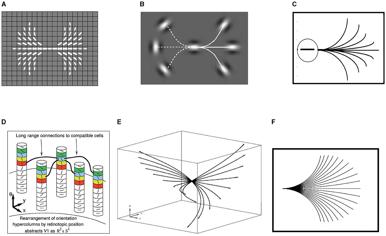
Figure 5. (A) Examples of the compatibilities around the central point of the image, derived from planar co-circularity. Brightness encodes compatibility values. Figure adapted from Ben-Shahar and Zucker (2004). (B) Starting from the central initial oriented point, the solid line indicates a configuration between the patches where the association exists while the dashed line indicates a configuration where it does not. Figure adapted from Field et al. (1993). (C) Association field of Field, Hayes, and Hess. Figure adapted from Field et al. (1993). (D) Orientation columns of cells in (x, y, θ) coordinates. Long-range horizontal connections between cells relate an orientation signal at position (x, y, θ) to another orientation at (x′, y′, θ′). Figure adapted from Ben-Shahar and Zucker (2004). (E) Horizontal integral curves in ℝ² × 𝕊¹ generated by the sub-Riemannian model (Citti and Sarti, 2006). (F) Projection of the fan of the integral curves in the (x, y) plane. Figure adapted from Citti and Sarti (2006).

Following the model of Citti and Sarti (2006), the set of simple cells' RPs can be obtained via translations along a vector (x, y)^T and rotation around angle θ from a unique “mother” profile φ₀(ξ, η):

$\begin{array}{ll}{\phi }_0(\xi ,\eta )=exp\left(\frac{2\pi i\xi }{\lambda }\right)exp\left(-\frac{{\xi }^2+{\eta }^2}{2{\sigma }^2}\right),& (8)\end{array}$

This RP is a Gabor function with even real part and odd imaginary part (Figure 7A). Translations and rotations can be expressed as:

$\begin{array}{ll}{T}_{(x,y,\theta )}(\xi ,\eta )=\left(\begin{array}{ll}cos\theta & -sin\theta \\ sin\theta & cos\theta \end{array}\right)\left(\begin{array}{l}\xi \\ \eta \end{array}\right)+\left(\begin{array}{l}x\\ y\end{array}\right),& (9)\end{array}$

where T_{(x, y, θ)} denotes the action of the group of rotations and translations SE(2) on ℝ². This group operation associates to every point (ξ, η) a new point $(\tilde{x},ỹ)$, according to the law $(\tilde{x},ỹ)=T_{(x,y,\theta )}(\xi ,\eta )$. Hence, a general RP can be expressed as

$\begin{array}{ll}{\phi }_{(x,y,\theta )}(\xi ,\eta )={\phi }_0(T_{(x,y,\theta )}^{-1}(\xi ,\eta )),& (10)\end{array}$

and this represents the action of the group SE(2) on the set of receptive profiles.

The retinal plane $\mathcal{R}$ is identified with the ℝ² plane, whose coordinates are (x, y). When a visual stimulus $I:\mathcal{R}\to {ℝ}^{+}$ of intensity I(x, y) activates the retinal layer, the neurons centered at every point (x, y) produce an output O(x, y, θ), modeled as the integral of the signal I with the set of Gabor filters:

$\begin{array}{ll}O(x,y,\theta )={\displaystyle {\int }_{\mathcal{R}}}{\phi }_{\left\{x,y,\theta \right\}}(\xi ,\eta )I(\xi ,\eta )d\xi d\eta ,& (11)\end{array}$

where the function I represents the retinal image.

For (x, y) fixed, we will denote $\bar{\theta }$ the point of maximal response:

$\begin{array}{ll}{\displaystyle \underset{\theta }{max}}\left|O(x,y,\theta )\right|=\left|O(x,y,\bar{\theta })\right|.& (12)\end{array}$

We will then say that the point (x, y) is lifted to the point $(x,y,\bar{\theta })$. This is extremely important conceptually to understand our geometry: it illustrates how an image point, evaluated against a simple cell RP, is lifted to a “cortical” point by introducing the orientation explicitly. If all the points of the image are lifted in the same way, the level lines of the 2D image I are lifted to new curves in the 3D cortical space $(x,y,\bar{\theta })$.

We shall now recall a model of the long range connectivity which allows propagation of the visual signal from one cell in a column to another cell in a nearby column. This is formalized as a set of directions for moving in the cortical space $(x,y,\bar{\theta })$, in the sense of vector fields. This is important because it will be necessary to move within this space, across both positions and orientations.

To begin, in the right hand side of the Equation (11) the integral of the signal with the real and imaginary part of the Gabor filter is expressed. The two families of cells have different shapes, hence they detect (or play a role in detecting) different features. Since the odd-symmetry cells suggest boundary detection, we concentrate on them, but this is a mathematical simplification. The output of a simple cell can then be locally approximated as O(x, y, θ) = −X_3,p(I_σ)(x, y), where p = (x, y, θ) ∈ SE(2), I_σ is a smoothed version of I, obtained by convolving it with a Gaussian kernel, and

$\begin{array}{ll}{X}_{3,p}=-sin\theta {\partial }_x+cos\theta {\partial }_y,& (13)\end{array}$

is the directional derivative in the direction ${\overrightarrow{X}}_{3,p}={(-sin\theta ,cos\theta ,0)}^T$. From now on, we will denote (by a slight abuse of notation) ${\omega }^{\star }:={\overrightarrow{X}}_{3,p}$ to remind the reader familiar with the language of 1-forms the correspondence of these quantities, and the relation with the Hodge star operator.⁶

Now, think of vector fields as defining a coordinate system at each point in cortical space. Then, in addition to above, the vector fields orthogonal to X_3,p are:

$\begin{array}{ll}{X}_{1,p}=cos\theta {\partial }_x+sin\theta {\partial }_y,X_{2,p}={\partial }_{\theta }& (14)\end{array}$

and they define a 2-dimensional admissible tangent bundle⁷ to ℝ² × 𝕊¹. One can define a scalar product on this space by imposing the orthonormality of X_1,p and X_2,p: this determines a sub-Riemannian structure on ℝ² × 𝕊¹.

The visual signal propagates, in an anisotropic way, along cortical connectivity and connects more strongly cells with comparable orientations. This propagation has been expressed by the geometry just developed and 2-dimensional contour integration. This is the neural explanation of the Gestalt law of good continuation (Koffka, 1963; Kohler, 1967). It can be directly expressed as co-circularity in the plane (Parent and Zucker, 1989), to describe the consistency and the compatibility of neighboring oriented points, in accordance with specific values of curvature. An example of these compatibilities can be found in Figure 5A. It is complemented by psychophysical experiments, e.g., Uttal, 1983; Smits and Vos, 1987; Ivry et al., 1989. In particular, Field et al. (1993) describe the association rules for 2-dimensional contour integration, introducing the concept of association fields. A representation of these connections can be found in Figures 5B, C. Note that this is equivalent to the union (over curvature) in Parent and Zucker (1989). Neurophysiological studies (Blasdel, 1992; Malach et al., 1993; Bosking et al., 1997; Schmidt et al., 1997; Hess et al., 2014) suggest that the cortical correlate of the association field is the long-range horizontal connectivity among cells of similar (but not necessarily identical) orientation preference.

Based on these findings, Citti and Sarti (2006) modeled cortical propagation as propagation along integral curves of the vector fields X₁ and X₂, namely curves γ:[0, T]⊂ℝ → ℝ² × 𝕊¹ described by the following differential equation:

$\begin{array}{ll}\dot{\gamma }(t)={\overrightarrow{X}}_{1,\gamma (t)}+k{\overrightarrow{X}}_{2,\gamma (t)},t\in \left[0,T\right],& (15)\end{array}$

obtained by varying the parameter k ∈ ℝ. (k acts analogously as curvature.) An example of these curves is in Figure 5E. Their 2D projection is a close approximation of the association fields (Figure 5F).

A related model has been proposed by Duits et al. (2013). They study the geodesics of the sub-Riemannian structure to take into account all appropriate end-conditions of association fields.

2.2.2 Generalizing co-circularity for stereo

The concept of co-circularity in ℝ² has been developed by observing that a bidimensional curve γ can be locally approximated at 0 via the osculating circle.⁸ Alibhai and Zucker (2000), Li and Zucker (2003), and Li and Zucker (2006) generalize this concept with the Frenet differential geometry of a three dimensional curve.

While in the two-dimensional case the approximation of the curve using the Frenet 2D basis causes the curvature to appear in the coefficient of the Taylor series development (1st order), in the three-dimensional case the coefficients involve both the curvature and torsion. So, in Alibhai and Zucker (2000) the authors propose heuristically to generalize the osculating circle for space curves with an osculating helix, with a preference for r₃-helices to improve stability in terms of camera calibration. In this way the orientation disparity is encoded in the behavior of the helix in the 3D space: there is no difference in orientation in the retinal planes if the helix is confined to be in the fronto-parallel plane (the helix becomes a circle); otherwise moving along the 3D curves the retinal projections have different orientations.

In Li and Zucker (2003, 2006) they observe that, by introducing the curvature variable as a feature in the two monocular structures, and assuming correspondence, it is possible to reconstruct the 3D Frenet geometry of the curve, starting from the two-dimensional Frenet geometry, up to the torsion parameter. In particular, they prove:

Proposition 2.1. Given two perspective views of a 3D space curve with full calibration, the normal N and curvature k at a curve space point are uniquely determined from the positions, tangents, and curvatures of its projections in two images. Thus the Frenet frame {T, N, B} and curvature k at the space point can be uniquely determined.

Hence, using the knowledge of the Frenet basis together with the fundamental addition of the curvature variable, Zucker et al. applied the concept of transport. This allowed moving the 3D Frenet frame in a consistent way with the corresponding 2D Frenet structures of the left and right retinal planes, to establish stereo correspondence between pairs of (left and right) pairs of tangents (see Figure 6B).

Figure 6

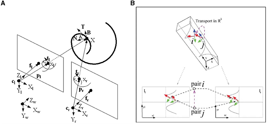
Figure 6. (A) Geometrical setup of Proposition 2.1. The spiral curve 3D projects in the left and right retinal planes together with the Frenet structure. (B) Stereo correspondence between pairs of (left-right) pairs of tangents. Both figures are taken from Li and Zucker (2006).

Remark 2.3. The model that we propose in this paper is related to, but differs from, what has just been stated. In particular, to remain directly compatible with the previous neuro-geometric model, we will work only with the monocular variables of position and orientation. Rather than using curvature directly, we shall assume that these variables are encoded within the connections; mathematically they appear as parameters. A theoretical result of our model is that the heuristic assumption regarding the r₃-helix can now be established rigorously.

Let us also mention the paper (Abbasi-Sureshjani et al., 2017), where the curvature was considered as independent variable and helices have been obtained in the 2D space.

3 The neuromathematical model for stereo vision

Here, we do not want to directly impose a co-circularity property: our scope is to model the behavior of binocular cells, and deduce properties of propagation, which will ultimately induce a geometry of 3D good continuation laws.

3.1 Binocular profiles

Binocular neurons receive inputs from both the left and right eyes. To facilitate calculations, we assume these inputs are first combined in simple cells in the primary visual cortex, a widely studied approach (Anzai et al., 1999b; Cumming and DeAngelis, 2001; Menz and Freeman, 2004; Kato et al., 2016). It provides a first approximation in which binocular RPs are described as the product of monocular RPs; see Figure 7. This model is clearly an oversimplification, in several senses. First, it leaves out the more refined receptive fields discussed in Section 1.3. Second, it leaves out the role for complex cells (Sasaki et al., 2010). Third, it leaves out different ways to get the position and orientation information, such as eye fixations (Intoy et al., 2021). And fourth, it avoids the delicate question of whether the max operation over a column (Equation 12) truly captures a tangent element. Nevertheless, since our focus is geometric, it does capture all of the necessary ingredients and simplifies computations.

Figure 7

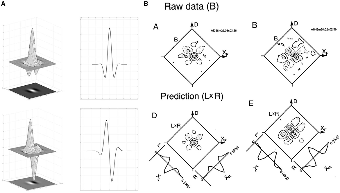
Figure 7. (A) Even (top) and odd (bottom) part of Gabor function: the surface of the two-dimensional filters, their common bi-dimensional representation and a mono-dimensional section. (B) Comparisons between binocular interaction RPs and the product of left and right eye RPs, where left and right RPs are shown in image (A). Binocular interaction RPs (Raw data) of a cell is shown on the top row. Contour plots for the product of left and right eye RPs (L × R) are shown in the bottom row along with 1-dimensional profiles of the left (L) and right (R) eye RPs. Figure adapted from Anzai et al. (1999b).

This binocular model allows us to define disparity and frontoparallel coordinates as

$\begin{array}{ll}\{\begin{array}{l}d=\frac{x_L-x_R}{2}\\ x=\frac{x_R+x_L}{2},\end{array}& (16)\end{array}$

perfectly in accordance with the introduction of cyclopean coordinates in (4). In this way (x, y, d) correspond to the neural correlate of (r₁, r₂, r₃), via the change of variables (5).

3.2 The cortical fiber bundle of binocular cells

The hypercolumnar structure of monocular simple cells (orientation selective) has been described as a jet fiber bundle in the works of Petitot and Tondut (1999), among many others. We concentrate on the fiber bundle ℝ² × 𝕊¹, with fiber 𝕊¹; see, e.g., Ben-Shahar and Zucker, 2004 among many others.

In our setting, the binocular structure is based on monocular ones; recall the example illustrations from the Introduction. In particular, for each cell on the left eye there is an entire fiber of cells on the right, and vice versa, for each cell on the right there is an entire fiber of cells on the left. This implies that the binocular space is equipped with a symmetry that involves the left and right structures, allowing us to use the cyclopean coordinates (x, y, d) defined in (16).

Hence, we define the cyclopean retina $\mathcal{R}$, identified with ℝ², endowed with coordinates (x, y). The structure of the fiber is $\mathcal{F}=ℝ\times S^1\times S^1$, with coordinates $(d,{\theta }_L,{\theta }_R)\in \mathcal{F}$. The total space is defined in a trivial way, $\mathcal{E}=\mathcal{R}\times \mathcal{F}={ℝ}^2\times ℝ\times S^1\times S^1$, and the projection $\pi :\mathcal{E}\to \mathcal{R}$ is the trivial projection π(x, y, d, θ_L, θ_R) = (x, y). The preimage of the projection ${\mathcal{E}}_{(x,y)}:={\pi }^{-1}(\left\{(x,y)\right\})$, for every $(x,y)\in \mathcal{R}$, is isomorphic to the fiber $\mathcal{F}$, and the local trivialization property is naturally satisfied.

A schematic representation can be found in Figure 8. The base has been depicted as 1-dimensional, considering the restriction ${\mathcal{R}}_{|x}$ of the cyclopean retina $\mathcal{R}$ on the coordinate x. The left image displays only the disparity component of the fiber $\mathcal{F}$, encoding the relationships between left and right retinal coordinates. The right image shows the presence of the left and right monodimensional orientational fibers.

Figure 8

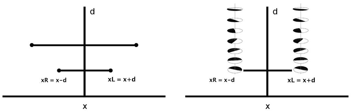
Figure 8. Left: schematic representation of the fiber bundle in two dimension, with relationships between left and right retinal coordinates. Right: representation of the selection of a whole fiber of left and right simple cells, for every x and for every d.

3.3 Binocular energy model

To simplify calculations, as stated in the Introduction, we follow the classical binocular energy model (Anzai et al., 1999b) for binocular RPs. The basic idea is a binocular neuron receives input from each eye; if the sum O_L + O_R of the inputs from the left and right eye is positive, the firing rate of the binocular neuron is proportional to the square of the sum, and it vanishes, if the sum of the inputs is negative:

$\begin{array}{ll}{O}_B={(Pos(O_L+O_R))}^2,& (17)\end{array}$

with Pos(x) = max{x, 0}, O_B the binocular output.

If O_L + O_R > 0, then the output of the binocular simple cell can be explicitly written as $O_B=O_L^2+O_R^2+2O_L{O}_R$. The first two terms represent responses due to monocular stimulation while the third term 2O_LO_R can be interpreted as the binocular interaction term.

The activity of a cell is then measured from the output and will be strongest at points that have a higher probability of matching each other. The maximum value over d of this quantity is the extracted disparity.

It is worth noting that neurophysiological computations of binocular profiles displayed in Figure 7B assume the mono-dimensionality of the monocular receptive profile, ignoring information about orientation of monocular simple cells. However, this information will be needed to encode different types of orientation disparity.

Remark 3.1 (Orientation matters). In 2001, the authors of Bridge et al. (2001) conducted investigations on the response of binocular neurons to orientation disparity, by extending the energy model of Anzai, Ohzawa, and Freeman to incorporate binocular differences in receptive-field orientation. More recently, the difference between orientations in the receptive fields of the eyes has been confirmed (Sasaki et al., 2010).

The binocular energy model is a type of minimal model. It serves as a starting point, allowing the combination of monocular inputs. But is not sufficient to solve the stereo-matching problem.

Remark 3.2 (Connections). It is argued in Samonds et al. (2013) and Parker et al. (2016) that, in addition to the neural mechanisms that couple characteristics (such as signals, stimuli, or particular features) relating the left and right monocular structures, there must be a system of connections between binocular cells, which characterizes the processing mechanism of stereo vision; see also Samonds et al. (2013) in particular.

3.4 Differential interpretation of binocular RPs

It is possible to write the interaction term O_LO_R coming from (17), in terms of the left and right receptive profiles:

$\begin{array}{ll}\begin{array}{l}{O}_L{O}_R={\displaystyle \int }{\phi }_{{\theta }_L,x_L,y}({\tilde{x}}_L,{ỹ}_L)I_L({\tilde{x}}_L,{ỹ}_L)d{\tilde{x}}_{L}d{ỹ}_L\\ {\displaystyle \int }{\phi }_{{\theta }_R,x_R,y}({\tilde{x}}_R,{ỹ}_R)I_R({\tilde{x}}_R,{ỹ}_R)d{\tilde{x}}_{R}d{ỹ}_R\\ ={\displaystyle \int \int }{\phi }_{{\theta }_L,x_L,y}({\tilde{x}}_L,{ỹ}_L){\phi }_{{\theta }_R,x_R,y}({\tilde{x}}_R,{ỹ}_R)I_L({\tilde{x}}_L,{ỹ}_L)\\ I_R({\tilde{x}}_R,{ỹ}_R)d{\tilde{x}}_{R}d{ỹ}_{R}d{\tilde{x}}_{L}d{ỹ}_L.\end{array}& (18)\end{array}$

If we fix $({\tilde{x}}_R,{ỹ}_R,{\tilde{x}}_L,{ỹ}_L)$, we derive the expression of the binocular profiles φ_L,R = φ_{θR, xR, y}φ_{θL, xL, y} as the product of monocular left and right profiles. This is in accordance with the measured profiles of Figure 7B).

Proposition 3.1. The binocular interaction term can be associated with the cross product of the left and right directions defined through (13), namely ${\omega }_L^{\star }$ and ${\omega }_R^{\star }$ of monocular simple cells:

$\begin{array}{ll}{O}_L{O}_R={\omega }_L^{\star }\times {\omega }_R^{\star }.& (19)\end{array}$

Proof. The idea is that the binocular output is the combined result of the left and right actions of monocular cells, thus identifying a direction in the space of cyclopean coordinates. The detailed proof of this proposition can be found in Appendix B (Supplementary material).     □

To better understand the geometrical idea behind Proposition 3.1, we recall that the retinal coordinates can be expressed in terms of cyclopean coordinates (4) as x_R = x − d and x_L = x + d, and so we can write ${\omega }_L^{\star }$ and ${\omega }_R^{\star }$ in the 3D space of coordinates (x, y, d) as:

$\begin{array}{ll}\begin{array}{l}{\omega }_R^{\star }={(-sin{\theta }_R,cos{\theta }_R,sin{\theta }_R)}^T\\ {\omega }_L^{\star }={(-sin{\theta }_L,cos{\theta }_L,-sin{\theta }_L)}^T.\end{array}& (20)\end{array}$

We define ${\omega }_{bin}:={\omega }_L^{\star }\times {\omega }_R^{\star }$ as the natural direction characterizing the binocular structure:

$\begin{array}{ll}{\omega }_{bin}=\left(\begin{array}{l}sin({\theta }_R+{\theta }_L)\\ 2sin{\theta }_{R}sin{\theta }_L\\ sin({\theta }_R-{\theta }_L)\end{array}\right).& (21)\end{array}$

Remark 3.3. The vector ω_bin of Equation (21) can be interpreted as the intersection of the orthogonal spaces defined with respect to ${\omega }_R^{\star }$ and ${\omega }_L^{\star }$ when expressed in cyclopean coordinates (x, y, d). More precisely, if

$\begin{array}{ll}\begin{array}{l}{({\omega }_L^{\star })}^{\perp }=\text{span}\left\{(\begin{array}{l}cos{\theta }_L\\ sin{\theta }_L\\ 0\end{array}),(\begin{array}{l}-1\\ 0\\ 1\end{array})\right\},\\ {({\omega }_R^{\star })}^{\perp }=\text{span}\left\{(\begin{array}{l}cos{\theta }_R\\ sin{\theta }_R\\ 0\end{array}),(\begin{array}{l}1\\ 0\\ 1\end{array})\right\}\end{array}& (22)\end{array}$

then

$\begin{array}{ll}{\omega }_{bin}={({\omega }_L^{\star })}^{\perp }\cap {({\omega }_R^{\star })}^{\perp }.& (23)\end{array}$

The result of the intersection of these monocular structures identifies a direction, as shown in Figure 9A.

Figure 9

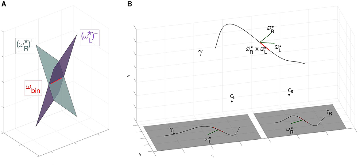
Figure 9. (A) Direction detected by ω_bin through the intersection of left and right planes generated by ${({\omega }_R^{\star })}^{\perp }$ and ${({\omega }_L^{\star })}^{\perp }$. Red vector corresponds to the associated 2-form ω_bin. (B) Three dimensional reconstruction of the space from retinal planes. The 1- forms ${\omega }_L^{\star }$ and ${\omega }_R^{\star }$ are identified with the normal to the curves γ_L and γ_R. Their three dimensional counterpart ${\tilde{\omega }}_L^{\star }$ and ${\tilde{\omega }}_R^{\star }$ identify the tangent vector to the curve γ:ℝ → ℝ³ by the cross product ${\tilde{\omega }}_L^{\star }\times {\tilde{\omega }}_R^{\star }$.

We earlier showed that the result of the action of a monocular odd simple cell is to select directions for the propagation of information. We now combine these, for the two eyes, to show that in the three-dimensional case the binocular neural mechanisms also lead to a direction. We will see in the next sections that this direction is the direction of the tangent vector to the 3D stimulus, provided points are corresponding.

3.5 Compatibility with stereo geometry

We consider the direction characterizing the binocular structure ω_bin defined in (21) and we show that it can be associated with the 3D tangent vector to the 3D curve. The idea is that this tangent vector is orthogonal both to ${\omega }_R^{\star }$ and to ${\omega }_L^{\star }$, and therefore it has the direction of the vector product ${\omega }_L^{\star }\times {\omega }_R^{\star }$.

Precisely, we consider the normalized tangent vector t_L and t_R on retinal planes

$\begin{array}{ll}{t}_R={(cos{\theta }_R,sin{\theta }_R)}^T{t}_L={(cos{\theta }_L,sin{\theta }_L)}^T,& (24)\end{array}$

to the points (x_R, y) and (x_L, y) respectively. Taking into account that f is the focal coordinate of the retinal planes in ℝ³, then we associate to these points the correspondents in ℝ³, namely ${\tilde{m}}_L={(x_L-c,y,f)}^T$, ${\tilde{m}}_R={(x_R+c,y,f)}^T$. Applying Equation (7), it is possible to derive the tangent vector of the three dimensional contour:

$\begin{array}{ll}\begin{array}{l}{U}_{t_L}=P_L^{-1}{\tilde{m}}_L\times P_L^{-1}{\tilde{t}}_L=\left(\begin{array}{l}{x}_L\\ y_L\\ f\end{array}\right)\times \left(\begin{array}{l}cos{\theta }_L\\ sin{\theta }_L\\ 0\end{array}\right)\\ =\left(\begin{array}{l}-fsin{\theta }_L\\ fcos{\theta }_L\\ x_{L}sin{\theta }_L-y_{L}cos{\theta }_L\end{array}\right),\\ U_{t_R}=P_R^{-1}{\tilde{m}}_R\times P_R^{-1}{\tilde{t}}_R=\left(\begin{array}{l}{x}_R\\ y_R\\ f\end{array}\right)\times \left(\begin{array}{l}cos{\theta }_R\\ sin{\theta }_R\\ 0\end{array}\right)\\ =\left(\begin{array}{l}-fsin{\theta }_R\\ fcos{\theta }_R\\ x_{R}sin{\theta }_R-y_{R}cos{\theta }_R\end{array}\right),\end{array}& \left(25\right)\end{array}$

and the tangent direction is recovered by

$\begin{array}{l}{U}_{t_L}\times U_{t_R}=\end{array}$

$\begin{array}{ll}f\left(\begin{array}{l}\frac{x_L+x_R}{2}sin({\theta }_R-{\theta }_L)-\frac{x_R-x_L}{2}sin({\theta }_L+{\theta }_R)\\ ysin({\theta }_R-{\theta }_L)-(x_R-x_L)(cos({\theta }_R-{\theta }_L)-cos({\theta }_L+{\theta }_R))\\ fsin({\theta }_R-{\theta }_L)\end{array}\right)& (26)\end{array}$

If we define

$\begin{array}{ll}{\tilde{\omega }}_L^{\star }:=\frac{d}{fc}{U}_{t_L},{\tilde{\omega }}_R^{\star }:=\frac{d}{fc}{U}_{t_R}& (27)\end{array}$

and the corresponding 2 form ${\omega }_{{ℝ}^3}:={\tilde{\omega }}_L^{\star }\times {\tilde{\omega }}_R^{\star }$, using the change of variables (16) we observe that:

$\begin{array}{ll}{\tilde{\omega }}_L^{\star }={\omega }_L^{\star },{\tilde{\omega }}_R^{\star }={\omega }_R^{\star },{\omega }_{{ℝ}^3}={\omega }_{bin},& (28)\end{array}$

up to a scalar factor. See Appendix C (Supplementary material) for explicit computation.

In this way, the disparity binocular cells couple in a natural way positions, identified with points in ℝ³, and orientations in 𝕊², identified with three-dimensional unitary tangent vectors. As already observed in Remark 3.2, the geometry of the stereo vision is not solved only with these punctual and directional arguments, but there is the need to take into accounts suitable type of connections. In Alibhai and Zucker (2000); Li and Zucker (2003, 2006), Zucker et al. proposed a model that considered the curvature of monocular structures as an additional variable. Instead, we propose to consider simple monocular cells selective for orientation, and to insert the notion of curvature directly into the definition of connection. It is therefore natural to introduce the perceptual space via the manifold ℝ³ ⋊ 𝕊², in line with the theoretical toolbox proposed in Miolane and Pennec (2016) to generalize 2D neurogeometry to 3D images, and adapt this framework to our problem, looking for appropriate curves.

3.6 A perceptual model in the space of 3D position-orientation

We now derive the objects in Figure 3A. We have clarified (end of Section 3.5) that binocular cells are parameterized by points in ℝ³, and orientations in 𝕊². An element ξ of the space ℝ³ ⋊ 𝕊² it is defined by a point p = (p1, p2, p3) in ℝ³ and an unitary vector n ∈ 𝕊². Since the topological dimension of this geometric object is 2, we introduce the classical spherical coordinates (θ, φ) such that $n=(n_1,n_2,n_3)\in S^2$ can be parameterized as:

$\begin{array}{ll}\begin{array}{l}{n}_1=cos\theta sin\phi \\ n_2=sin\theta sin\phi \\ n_3=cos\phi \end{array}& (29)\end{array}$

with θ ∈ [0, 2π] and φ ∈ (0, π). The ambiguity that arises using local coordinate chart is overcome by the introduction of a second chart, covering the singular points.

Translations and rotations are expressed using the group law of the three-dimensional special Euclidean group SE(3), defining the group action

$\begin{array}{ll}\sigma :{ℝ}^3⋊{𝕊}^2\times 𝕊E(3)\to {ℝ}^3⋊S^2\text{s.t.}\sigma ((p,n),(q,R))=(Rp+q,Rn),& (30)\end{array}$

with (p, n) ∈ ℝ³ ⋊ 𝕊², (q, R) ∈ SE(3), namely R ∈ SO(3) tridimensional rotation, and q ∈ ℝ³.

3.6.1 Stereo sub-Riemannian geometry

The emergence of a privileged direction in ℝ³ (associated with the tangent vector to the stimulus) is the reason why we endow ℝ³ ⋊ 𝕊² with a sub-Riemannian structure that favors the direction in 3D identified by ω_bin.

Formally, we consider admissible movements in ℝ³ ⋊ 𝕊² described by vector fields:

$\begin{array}{ll}\begin{array}{l}{Y}_{{ℝ}^3,\xi }=sin\phi cos\theta {\partial }_1+sin\phi sin\theta {\partial }_2+cos\phi {\partial }_3\\ Y_{\theta ,\xi }=-\frac{1}{sin\phi }{\partial }_{\theta }\\ Y_{\phi ,\xi }={\partial }_{\phi }\end{array}& (31)\end{array}$

with ξ ∈ ℝ³ ⋊ 𝕊² for φ ≠ 0, φ ≠ π. The admissible tangent space⁹ at a point ξ

$\begin{array}{ll}{\mathcal{A}}_{\xi }:=\text{span}\{Y_{{ℝ}^3,\xi },Y_{\theta ,\xi },Y_{\phi ,\xi }\}& (32)\end{array}$

encodes the coupling between position and orientations, as remarked by Duits and Franken (2011). In particular, the vector field $Y_{{ℝ}^3}$ identifies the privileged direction in ℝ³, while Y_θ and Y_φ allow changing this direction, involving just orientation variables of 𝕊². The vector fields $\left\{Y_{{ℝ}^3},Y_{\theta },Y_{\phi }\right\}$ and their commutators generate the tangent space of ℝ³ ⋊ 𝕊² in a point, allowing to connect every point of the manifold using privileged directions (Hörmander condition). Furthermore, it is possible to define a sub-Riemannian structure by choosing a scalar product on the admissible tangent bundle $\mathcal{A}$: the simplest choice is to declare the vector fields $\left\{Y_{{ℝ}^3},Y_{\theta },Y_{\phi }\right\}$ orthonormal, considering on 𝕊² the distance inherited from the immersion in ℝ³ with the Euclidean metric.

3.6.2 Change of variables

We have already expressed the change of variable in the variables (x, y, d) to (r₁, r₂, r₃) in Equation (5). However, the cortical coordinates also contain the angular variables θ_R and θ_L which involve the introduction of the spherical coordinates θ, φ.

To identify a change of variable among these variables, we first introduce the function $(r_1,r_2,r_3,\theta ,\phi )\underset{}{\overset{F}{\to }}(x,y,d,{\theta }_L,{\theta }_R)$ :

$\begin{array}{l}F:ℝ⋊𝕊\to ℝ⋊𝕊\\ \left(\begin{array}{c}{r}_1\\ r_2\\ r_3\\ \theta \\ \phi \end{array}\right)\mapsto \left(\begin{array}{c}\frac{f{r}_1}{r_3}\\ \frac{f{r}_2}{r_3}\\ \frac{cf}{r_3}\\ {\tan }^{-1}(\frac{r_3\sin \theta \cos \phi -r_2\cos \phi }{r_3\cos \theta \sin \phi -(c+r_1)\cos \phi })\\ ta{n}^{-1}(\frac{r_3\sin \theta \cos \phi -r_2\cos \phi }{r_3\cos \theta \sin \phi -(c-r_1)\cos \phi }\end{array}\right),& (33)\end{array}$

where the retinal right angle ${\theta }_R={tan}^{-1}(\frac{r_{3}sin\theta cos\phi -r_{2}cos\phi }{r_{3}cos\theta sin\phi -(c+r_1)cos\phi })$ and the retinal left angle ${\theta }_L={tan}^{-1}(\frac{r_{3}sin\theta cos\phi -r_{2}cos\phi }{r_{3}cos\theta sin\phi -(c-r_1)cos\phi })$ are obtained considering Equation (6).

Analogously, it is possible to define the change of variable $(x,y,d,{\theta }_L,{\theta }_R)\underset{}{\overset{G}{\to }}(r_1,r_2,r_3,\theta ,\phi )$:

$\begin{array}{ll}\begin{array}{cccc}G:& {ℝ}^3⋊{𝕊}^2& \to & {ℝ}^3⋊{𝕊}^2\\ \left(\begin{array}{c}x\\ y\\ d\\ {\theta }_R\\ {\theta }_L\end{array}\right)& \mapsto & \left(\begin{array}{c}\frac{cx}{d}\\ \frac{cy}{d}\\ \frac{cf}{d}\\ {tan}^{-1}\left(\frac{2sin{\theta }_{R}sin{\theta }_L}{sin\left({\theta }_R+{\theta }_L\right)}\right)\\ {tan}^{-1}\left(\frac{\sqrt{{sin}^2\left({\theta }_R+{\theta }_L\right)+4{sin}^2{\theta }_R{sin}^2{\theta }_L}}{sin\left({\theta }_R-{\theta }_L\right)}\right)\end{array}\right)\end{array},& \left(34\right)\end{array}$

where the angles $\theta ={tan}^{-1}(\frac{2sin{\theta }_{R}sin{\theta }_L}{sin({\theta }_R+{\theta }_L)})$ and $\phi ={tan}^{-1}(\frac{\sqrt{{sin}^2({\theta }_R+{\theta }_L)+4{sin}^2{\theta }_R{sin}^2{\theta }_L}}{sin({\theta }_R-{\theta }_L)})$ are obtained considering that $tan\theta =\frac{{({\overrightarrow{Y}}_{{ℝ}^3})}_2}{{({\overrightarrow{Y}}_{{ℝ}^3})}_1}$ and $tan\phi =\frac{\sqrt{{({\overrightarrow{Y}}_{{ℝ}^3})}_1^2+{({\overrightarrow{Y}}_{{ℝ}^3})}_2^2}}{{({\overrightarrow{Y}}_{{ℝ}^3})}_3}$.

3.6.3 Integral curves

The connectivity of the space is described by admissible curves of the vector fields spanning $\mathcal{A}$. In particular, a curve Γ:[0, T] → ℝ³ ⋊ 𝕊² is said to be admissible¹⁰ if:

$\begin{array}{ll}\dot{\Gamma }(t)\in {\mathcal{A}}_{\Gamma (t)},\leftrightarrow \dot{\Gamma }(t)=a(t){\overrightarrow{Y}}_{{ℝ}^3,\Gamma (t)}+b(t){\overrightarrow{Y}}_{\theta ,\Gamma (t)}+c(t){\overrightarrow{Y}}_{\phi ,\Gamma (t)},& (35)\end{array}$

where a, b, c are sufficiently smooth function on [0, T]. We will consider a particular case of these admissible curves, namely constant coefficient integral curves with a(t) = 1, since the vector field $Y_{{ℝ}^3}$ represents the tangent direction of the 3D stimulus (and so it never vanishes):

$\begin{array}{ll}\dot{\Gamma }(t)={\overrightarrow{Y}}_{{ℝ}^3,\Gamma (t)}+c_1{\overrightarrow{Y}}_{\theta ,\Gamma (t)}+c_2{\overrightarrow{Y}}_{\phi ,\Gamma (t)},& (36)\end{array}$

with c₁ and c₂ varying in ℝ.

These curves can be thought of in terms of trajectories in ℝ³ describing a movement in the ${\overrightarrow{Y}}_{{ℝ}^3}$ direction, which can eventually change according to ${\overrightarrow{Y}}_{\theta }$ and ${\overrightarrow{Y}}_{\phi }$. An example of the fan of integral curves was shown in the Introduction in Figure 3B.

It is worth noting that in the case described by coefficients c₁ and c₂ equal to zero, the 3D trajectories would be straight lines in ℝ³; by varying the coefficients c₁ and c₂ in ℝ, we allow the integral curves to follow curved trajectories, twisting and bending in all space directions.

Formally, the amount of “twisting and bending” in space is measured by introducing the notions of curvature and torsion. We then investigate how these measurements are encoded in the parameters of the family of integral curves, and what constraints have to be imposed to obtain different typologies of curves.

Remark 3.4. The 3D projection of the integral curves (36) will be denoted γ and satisfy $\dot{\gamma }(t)={(cos\theta (t)sin\phi (t),sin\theta (t)sin\phi (t),cos\phi (t))}^T$. Classical instruments of differential geometry let us compute the curvature and the torsion of the curve γ(t):

$\begin{array}{ll}\begin{array}{l}k=\sqrt{{(\dot{\phi })}^2+{sin}^2\theta {(\dot{\theta })}^2},\\ \tau =\frac{1}{k^2}(-cos\phi {sin}^2\phi {(\dot{\theta })}^3-sin\phi \dot{\phi }\ddot{\theta }+\dot{\theta }(-2cos\phi {(\dot{\phi })}^2+sin\phi \ddot{\phi })).\end{array}& (37)\end{array}$

Using the explicit expression of the vector fields Y_θ and Y_φ in Equation (36), we get

$\begin{array}{ll}\dot{\theta }=-\frac{c_1}{sin\phi },\dot{\phi }=c_2,& (38)\end{array}$

from which it follows that:

$\begin{array}{ll}\begin{array}{l}k=\sqrt{c_1^2+c_2^2}\\ \tau =c_{1}cotan\phi .\end{array}& (39)\end{array}$

Proposition 3.2. By varying the parameters c₁ and c₂ in (39) where we explicitly find solutions of (36), we have:

1. If $\phi =\frac{\pi }{2}$ then $k=\sqrt{c_1^2},\tau =0$, and so the family of curves (36) are circles of radius $1/c_1^2$ on the fronto-parallel plane r₃ = cost.

2. If φ = φ₀, with φ₀ ≠ π/2, then $k=\sqrt{c_1^2}$ and τ = c₁cotanφ₀, and so the family of curves (36) are r₃-helices.

3. If θ = θ₀ then $k=\sqrt{c_2^2}$, τ = 0, and so the family of curves (36) are circles of radius $1/c_2^2$ in the osculating planes.

Proof. The computation follows immediately from the computed curvature and torsion of (39) and classical results of differential geometry.     □

Remark 3.5. If we know the value of the curvature k, and we have one free parameter, c₂, in the definition of the integral curves (36), then we are in the setting of Proposition 2.1. In fact, the coefficient c₁ is obtained by imposing $c_1=\pm \sqrt{k^2-c_2^2}$, and in particular the component that remains to be determined is the torsion.

Examples of particular cases of the integral curves (36) according to Proposition 3.2 and Remark 3.5 are visualized in Figure 10.

Figure 10

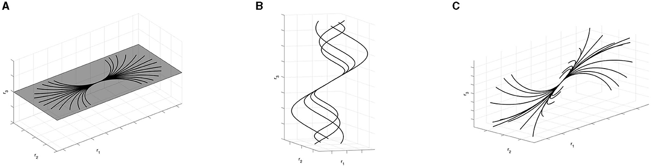
Figure 10. Examples of integral curves obtained varying parameters c₁ and c₂. (A) Arc of circles for φ = π/2. (B) r₃-helices for φ = π/3. (C) Family of curves with constant curvature k and varying torsion parameter.

4 Comparison with experimental data

Our sub-Riemannian model enjoys some consistency with the biological and psychophysical literature. We here describe some initial connections.

4.1 Biological connections

The foundation for building our sub-Riemannian model of stereo was a model of curve continuation, motivated by the orientation columns at each position. The connections between cells in nearby columns were, in turn, a geometric model of long-range horizontal connections in visual cortex (Bosking et al., 1997). In the Introduction we cartooned aspects of the cortical architecture that support binocular processing. Although the inputs are organized into ocular dominance bands, there is no direct evidence for “stereo columns” in V1 analogous to the monocular orientation columns. But such columns are not strictly necessary for our model. Rather, what is central is how information propagates. We showed in Figure 1C that there is evidence of long-range connections between binocular cells, and our model informs, abstractly, what information could propagate along these connections. Although less extensive than in the monocular case, some measurements are beginning to emerge that are informative.

The Grinwald group first established the presence of long-range connections between binocular cells (Malach et al., 1993) (see also Figure 11A), using biocytin. This is a molecule that is taken up by neurons, propagates directly along neuronal processes and is deposited at excitatory synapses. These results were refined, more recently, by the Fitzpatrick group (Scholl et al., 2022), using in vivo calcium imaging. As shown in Figure 1C the authors demonstrated both the monocular and the binocular inputs for stereo, and (not shown) the dependence on orientations.

Figure 11

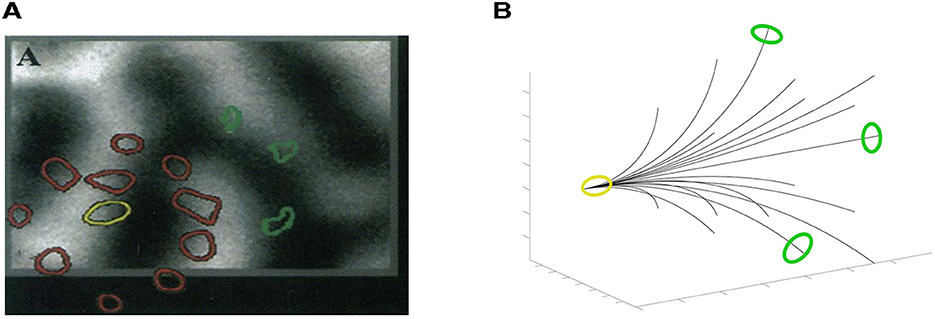
Figure 11. (A) A biocytin injection superimposed on a map of ocular dominance columns, image result from the work in Malach et al. (1993). Binocular zones are in the middle of monocular zones (coded in black and white). Starting from the injection site (yellow circle in the center of a binocular zone) the patches' propagation (red corresponds to dense while green to sparsely labeled) tends to avoid highly monocular sites, bypassing the centers of ocular dominance columns, and are located in binocular zones. (B) 3D interpretation of the physiological image (A).

More precisely, Malach et al. (1993) showed selective anisotripic connectivity among binocular regions: the biocytin tracer does not spread uniformly, but rather is highly directional with distance from the injection point. (This was the case with monocular biocytin injections as well.) Putting this together with Scholl et al. (2022), we interpret the anisotropy as being related to (binocular) orientation (Scholl et al., 2022), which is what the integral curves of our vector fields suggest. Our 3D association fields are strongly directional, and information propagates preferentially in the direction of (the starting point of) the curve. An example can be seen in Figure 11B, where the fan of integral curves (36) is represented, superimposed with colored patches, following the experiment proposed in Malach et al. (1993). We look forward to more detailed experiments along these lines.

4.2 Psychophysics and association fields

In this section, we show that the connections described by the integral curves in our model can be related to the geometric relationships from psychophysical experiments on perceptual organization of oriented elements in ℝ³; in other words, that our connections serve as a generalization of the concept of an association field in 3D.

4.2.1 Toward a notion of association field for 3D contours

The perception of continuity between two elements of position-orientation in ℝ³ has been studied experimentally. To start, Kellman, Garrigan, and Shipley (Kellman et al., 2005a,b) introduce 3D relatability, as a way to extend to 3D the experiments of Field, Hayes and Hess (Field et al., 1993) in 2D.

Particularly, in a system of 3D Cartesian coordinates, it is possible to introduce oriented edges E at the application point ${(r_1,r_2,r_3)}^T$ and with an orientation identified with the angles θ and φ. This orientation can be read, in our case, through the direction expressed by (cosθsinφ, sinθsinφ, cosφ)^T. For an initial edge E₀, with application point on the origin of the coordinate system (0, 0, 0)^T and orientation lying on the r₁-axis, described by θ = 0, φ = π/2, the range of possible orientations (θ, φ)¹¹ for 3D-relatable edges with E₀ is given by:

$\begin{array}{ll}{tan}^{-1}\left(\frac{r_2}{r_1}\right)\le \theta \le \frac{\pi }{2}\text{and}\frac{\pi }{2}\le \frac{3\pi }{2}-\phi \le {tan}^{-1}\left(\frac{r_3}{r_1}\right).& (40)\end{array}$

The bound on these equations identified with the quantity $\frac{\pi }{2}$ incorporates the 90 degree constraint in three dimensions, while the bounds defined by the inverse of the tangent express the absolute orientation difference between the reference edge E₀ and an edge positioned at the arbitrary oriented point E_{(r1, r2, r3)} so that its linear extension intersects E₀; see Kellman et al. (2005a,b) for further details.

Numerical simulations allow us to visually represent an example of the 3D positions and orientations that meet the 3D relatability criteria. Starting from an initial edge E₀ with endpoints in ${(p_{01},p_{02},p_{03})}^T$ and orientation on the e₁- axis, we represent for an arbitrary point ${(p_1,p_2,p_3)}^T$ the limit of the relatable orientation (θ, φ). Results are shown in Figure 12A.

Figure 12

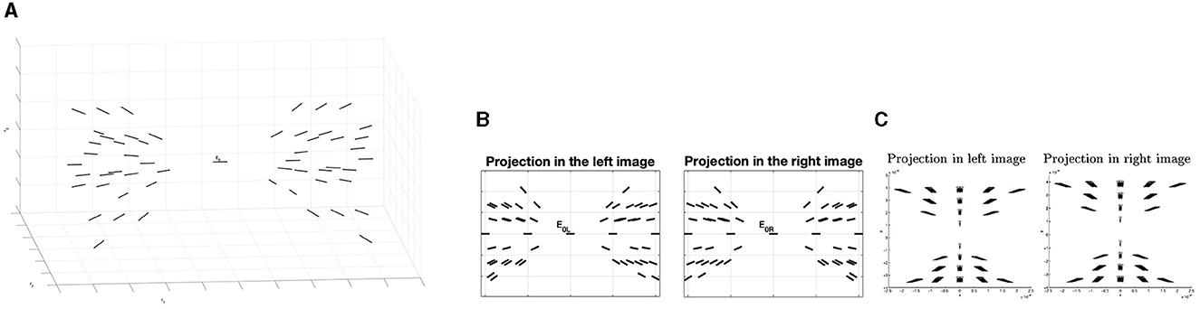
Figure 12. (A) Example of the fan of the 3D relatable edges with initial point E₀. (B) Example of 3D association field in the two left and right retinal planes, generated with the geometry of 3D relatability. (C) Example of 3D compatibility field of Alibhai and Zucker (2000).

Remark 4.1. By projecting on the retinal planes of the 3D fan of relatable points, it is possible to notice that these projections are in accordance with the notion of 3D compatibility field in Alibhai and Zucker (2000) (see Figures 12B, C).

Psychophysical studies, see Hess and Field (1995); Hess et al. (1997); Deas and Wilcox (2015), have investigated the properties of the curves that are suitable for connecting these relatable points. These curves are well-described as smooth and monotonic. In particular, using non-oriented contour elements for contours, Hess et al. (1997) indicate that contour elements can be effectively grouped based primarily on the good continuation of contour elements in depth. This statement is confirmed by the more recent work of Deas and Wilcox (2015) who, in addition, observe that detection of contours defined by regular depth continuity is faster than detection of discontinuous contours. All these results support the existence of depth grouping operations, arguing for the extension of Gestalt principles of continuity and smoothness in three dimensional space. Finally, on the relationship of the three-dimensional curves to 2-dimensional association fields, see Kellman et al. (2005b); Khuu et al. (2016). These authors have assumed that the strength of the relatable edges in the co-planar planes of E₀ must meet the relations of the bi-dimensional association fields of Field et al. (1993).

4.2.2 Compatibility with the sub-Riemannian model

To model the associations underlying the 3D perceptual organization discussed in the previous paragraph, we consider again the constant coefficient family of integral curves studied in (36):

$\begin{array}{ll}\dot{\Gamma }(t)={\overrightarrow{Y}}_{{ℝ}^3,\Gamma (t)}+c_1{\overrightarrow{Y}}_{\theta ,\Gamma (t)}+c_2{\overrightarrow{Y}}_{\phi ,\Gamma (t)},\text{with }{c}_1,c_2\in ℝ.& (41)\end{array}$

Importantly, these curves locally connect the association fan generated by the geometry of 3D relatability. In particular, Figure 13B shows the family of the horizontal curves connecting the initial point E₀ with 3D relatable edges (Figure 13A). These curves are computed using Matlab solver function ode45.

Figure 13

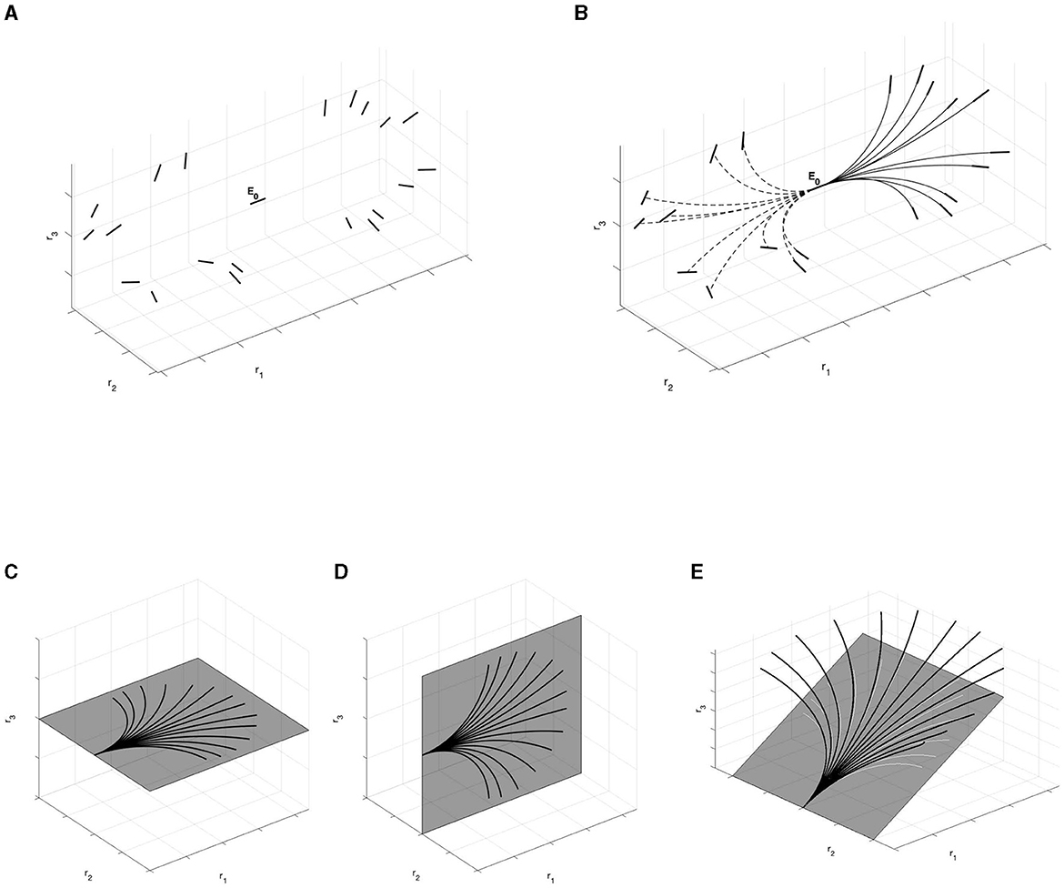
Figure 13. (A) 3D relatable edges displayed on the right of the initial edge E₀. Unrelatable 3D edges displayed on the left. (B) Horizontal integral curves with filled lines connect 3D relatable edges with initial point E₀. Horizontal integral curves with dotted lines do not connect 3D unrelatable edges. (C) Restriction of the fan of the integral curves on the e₁-e₂ plane. (D) Restriction of the fan of the integral curves on the e₁-e₃ plane. (E) Restriction of the fan at φ = φ₀. These curves (black lines) are not planar curves but helices. However, their projection (white lines) on the coplanar plane with initial edge satisfies the bidimensional constraints.

In analogy with the experiment of Field, Hayes, and Hess in Field et al. (1993), we choose to represent non-relatable edges to the left of the starting point E₀, while on the right are 3D relatable edges. So, filled lines of the integral curves indicate the correlation between the central horizontal element E₀ and the ones on its right, while dotted lines connect the starting point E₀ with elements not correlated with it, as represented on the left part of the image.

Restricting the curves on the neighborhood of co-planar planes with an arbitrary edge E, we have different cases. First, on the r₁-r₂ plane (fronto-parallel) and the r₁-r₃ plane we have arcs of circle, as proved with Proposition 3.2. Furthermore, for an arbitrary plane in ℝ³ containing an edge E, we observe that the curves generating with fixed angle φ are helices, and locally they satisfy the bidimensional constraint in the plane. Examples can be found in Figures 13C–E. In particular, the curves displayed in Figures 13C, D are well in accordance with the curves of the Citti-Sarti model, depicted in Figure 5.

One final connection with the psychophysical literature concerns how depth discrimination thresholds increase exponentially with distance (Burge, 2020 and references therein). This is related to how the fan of integral curves “spreads out” with distance (Figures 11, 12), which is also exponential. These notions are developed more fully in Bolelli et al. (2023a).

4.3 Integration of contours and stereo correspondence problem

Although the goal of this paper is not to solve the stereo correspondence problem, we can show how our geometry is helpful in understanding how to match left and right points and features. These ideas are developed more fully in Bolelli (2023).

Inspired by Hess and Field (1995), we consider a path stimulus γ interpreted as a contour, embedded in a background of randomly oriented elements: left and right retinal visual stimuli are depicted in Figure 14A. We perform an initial, simplified lift of the retinal images to a set Ω ⊂ ℝ³ ⋊ 𝕊². This set contains all the possible corresponding points, obtained by coupling left and right points which share the same y retinal coordinate, see Figure 14B. The set Ω contains false matches, namely points that do not belong to the original stimulus. It is the task of correspondence to eliminate these false matches.

Figure 14

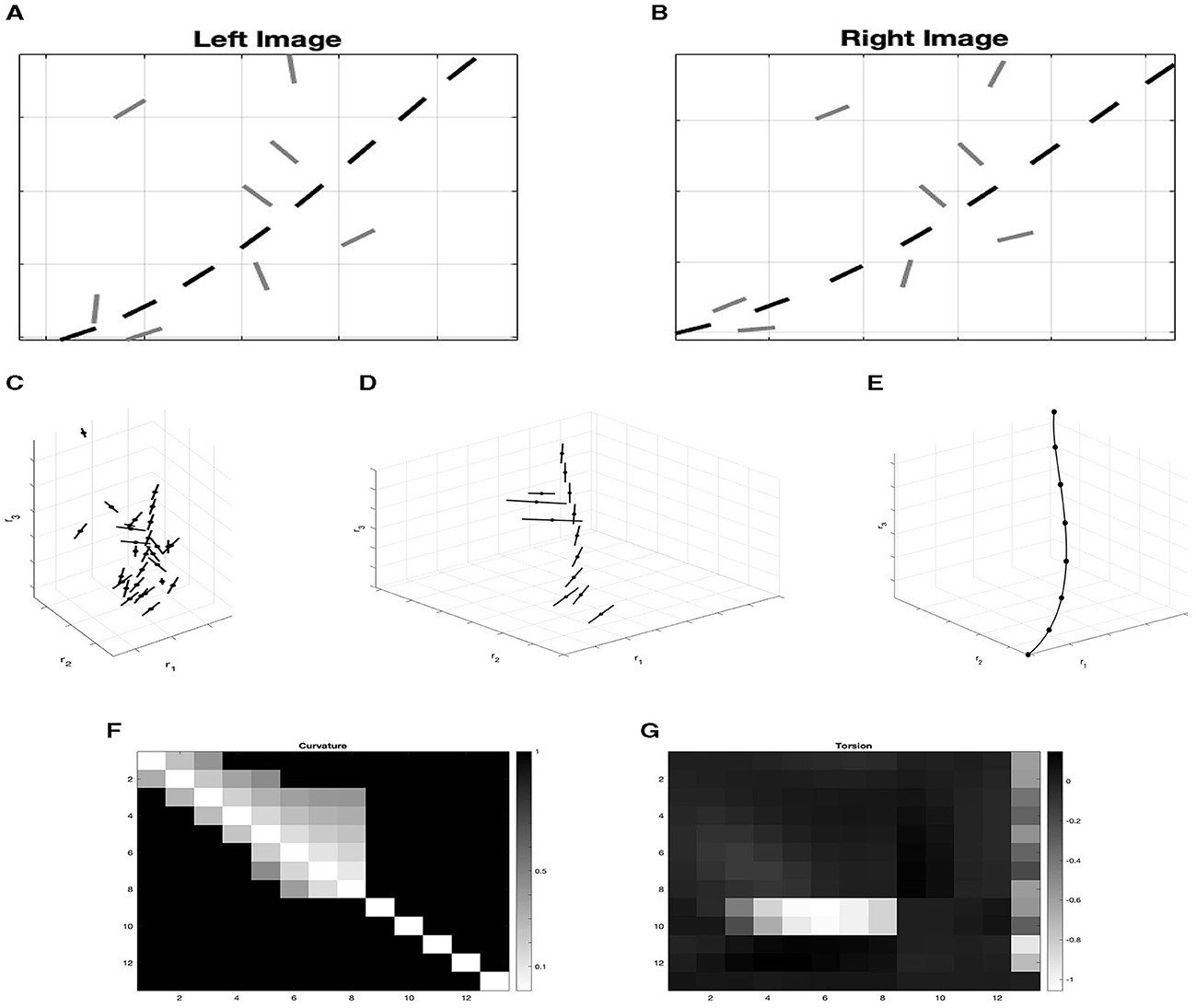
Figure 14. (A) Left and right retinal images of the set Ω. Black points are the projection of the point of the curve γ, while gray points are background random noise. (B) Lifting of the two left and right retinal images of image (A) in the space of position and orientation ℝ³ × 𝕊². (C) Selection of lifted points according to the binocular output. (D) Points of the stimulus γ connected by integral curves (36). (E, F) Matrices M which element M_ij represents the value of curvature/ torsion for every couple of points ξ_i, ξ_j. The first eight points correspond to points of the curve γ while the others are random noise. (E) Curvature matrix. (F) Torsion matrix.

We compute for every lifted point the binocular output O_B of Equation (17). This output can be seen as a probability measure that gives information on the correspondence of the pair of left and right points. We then simply evaluate which are the points with the highest probability of being in correspondence, applying a process of suppression of the non-maximal pairs over the fiber of disparity. In this way, noise points are removed (Figure 14C). We now directly exploit the Gestalt rule of good continuation by filtering out any couple of elements with high curvature. This qualitative rule could be quantitatively modeled by considering the statistics of distribution of curvature and torsion in natural 3D images (Geisler and Perry, 2009). The remaining noise elements are orthogonal to the directions of the elements of the curve that we would like to reconstruct. Calculating numerically the coefficients c₁ and c₂ of integral curves (36) that connect all the remaining pairs of points, we can obtain for every pair the value of curvature and torsion using (39).

Figures 14E, F show matrices M representing the values of curvature or torsion for every pair of points ξ_i, ξ_j in the element M_ij. In particular, we observe that random points are characterized by very high curvature and deviating torsion. So, by discarding these high values, we select only the three-dimensional points of the curve γ, which are well-connected by the integral curves, as shown in Figure 14D. This is in accordance with the idea developed in Alibhai and Zucker (2000); Li and Zucker (2003, 2006), where curvature and torsion provide constraints for reconstruction in 3D.

In this artificial example we assumed that local edge elements have already been detected. Our goal was simply proof-of-concept. To apply this approach to realistic images, of course, stages of edge detection would have to be adopted, for which there is a huge literature well outside the scope of our theoretical study.

5 Summary and conclusions

Understanding good continuation in depth, like good continuation for planar contours, can benefit from basic physiological constraints; from psychophysical performance measures, and from mathematical modeling. In particular, good continuation in the plane is supported by orientation selectivity and cortical architecture (orientation columns), by association field grouping performance, and by geometric modeling. We showed that the same should be true for good continuation in depth. However, while the psychophysical data may be comparable, the physiological data are weaker and the geometry of continuation is not as well-understood. In this paper, we introduced the neuro-geometry of stereo vision to fill this gap. It is strongly motivated by an analogical extension to 3D of 2D geometry, while respecting the psychophysics. In the end, it allowed us to be precise about the type of geometry that is relevant for understanding stereo abstractly, and concretely was highly informative toward the physiology. Although a “stereo columnar architecture” is not obvious from the anatomy, it is well-formed computationally.

Technically, we proposed a sub-Riemannian model on the space of position and orientation ℝ³ ⋊ 𝕊² for the description of the perceptual space of the neural cells involved. This geometrical structure favors the tangent direction of a 3D curve stimulus. The integral curves of the sub-Riemannian structure encode the notions of curvature and torsion within their coefficients, and are introduced to describe the connections between elements. This model can be seen as an extension in the three-dimensional scene of the 2-dimensional association field. In particular, the integral curves of the sub-Riemannian structure of the 3D space of position-orientation are exactly those that locally correspond to psychophysical association fields.

Although the goal of this paper is not to solve the stereo correspondence problem, we have seen how the geometry we propose is a good starting point to understand how to match left and right points and features. We used binocular receptive fields to prioritize orientation preferences and orientation differences under the assumption that neuronal circuitry has developed to facilitate the interpolation of contours in 3D space. On the other side, the neurogeometrical method has been coupled with a probabilistic methods for example in Sanguinetti et al. (2010) and Sarti and Citti (2015). Here, the authors studied an analogous problem for generation of perceptual units in monocular vision: they introduced stochastic differential equations, analogous to the integral curves of vector fields, and used its probability density as a kernel able to generate monocular perceptual units. In Montobbio et al. (2019), the probability kernel is built in a direction starting from the receptive fields. A future development of the model will consist in adapting the technique of Sarti and Citti (2015) to find the probability of the co-occurrence between two elements, and individuate percepts in 3D space. Individuation of percepts through harmonic analysis on the sub-Riemannian structure has been proposed in the past, both for 2D spatial stimuli (Sarti and Citti, 2015) and in 2D + time spatio-temporal stimuli (Barbieri et al., 2014a). It would be interesting to develop a similar analysis and extend it to stereo vision.

Data availability statement

The raw data supporting the conclusions of this article will be made available by the authors, without undue reservation.

Author contributions

All authors listed have made a substantial, direct, and intellectual contribution to the work and approved it for publication.

Funding

The author(s) declare financial support was received for the research, authorship, and/or publication of this article. MB, GC, and AS were supported by EU Project, GHAIA, Geometric and Harmonic Analysis with Interdisciplinary Applications, H2020-MSCA-RISE-2017. SZ was supported in part by US NIH EY031059 and by US NSF CRCNS 1822598.

Acknowledgments

The current article is part of the first named author's Ph.D. thesis (Bolelli, 2023) and a preprint version is available at Bolelli et al. (2023b).

Conflict of interest

The authors declare that the research was conducted in the absence of any commercial or financial relationships that could be construed as a potential conflict of interest.

Publisher's note

All claims expressed in this article are solely those of the authors and do not necessarily represent those of their affiliated organizations, or those of the publisher, the editors and the reviewers. Any product that may be evaluated in this article, or claim that may be made by its manufacturer, is not guaranteed or endorsed by the publisher.

Supplementary material

The Supplementary Material for this article can be found online at: https://www.frontiersin.org/articles/10.3389/fcomp.2023.1142621/full#supplementary-material

Footnotes

1. ^We are here being loose with language. By a tangent orientation in the left eye, we mean the orientation of a left-eye innervated column in V1.

2. ^Of course we need to take into account the difficulty of measurements of coupled position-orientation variables for small difference of angle and position. This is due to the well-known intrinsic uncertainty of measurement in the non-commutative group of position and orientation (Barbieri et al., 2012).

3. ^The crucial point is that the curves demonstrate locally quadratic (not linear) behavior.

4. ^Portions of this material were presented at Bolelli et al. (2023a).

5. ^The Jacobian matrix (_JΠ)p evaluated at point p represents how to project displacement vectors (in the sense of derivatives or velocities or directions). In details, if $\dot{\gamma }(t)$ is the displacement vector in ℝ³, then the matrix product ${(J_{\Pi })}_{\gamma (t)}\dot{\gamma }(t)$ is another displacement vector, but in ℝ². In other words, the Jacobian matrix is the differential of Π at every point where Π is differentiable; common notation includes J_Π or DΠ.

6. ^The purpose of introducing this notation is also to motivate an implication of the mathematical model in Citti and Sarti (2006); see Appendix B.2.1 (Supplementary material) for explanation.

7. ^as defined in Appendix A3 (Supplementary material).

8. ^Locally, a curve can be approximated by its osculating circle and, at a slightly larger scale, by the integral (parabolic) curve through the first two Taylor terms. The first approximation is co-circularity; the second is a parabolic curve. The second is an accurate model over large distances; see discussion in Section 1.3. However, since in this paper we are working over small distances and with cortical sampling (Figure 2), there is essentially no difference between them; see Figure 22.4 in Zucker (2006) and Sanguinetti et al. (2010) for a direct comparison.

9. ^see Appendix A (Supplementary material) for the definition of admissible tangent space.

10. ^sometimes the term horizontal is preferred.

11. ^The angle φ here has been modified to be compatible with our set of coordinates. The relationship between the angle $\tilde{\phi }$ in works (Kellman et al., 2005a,b) can be expressed as : $\tilde{\phi }=acos(sin\phi )+\pi$.

References

Abbasi-Sureshjani, S., Favali, M., Citti, G., Sarti, A., and ter Haar Romeny, B. M. (2017). Curvature integration in a 5D kernel for extracting vessel connections in retinal images. IEEE Trans. Image Process. 27, 606–621. doi: 10.1109/TIP.2017.2761543

PubMed Abstract | Crossref Full Text | Google Scholar

Agrachev, A., Barilari, D., and Boscain, U. (2019). A Comprehensive Introduction to Sub-Riemannian Geometry. Vol. 181. Cambridge: Cambridge University Press. doi: 10.1017/9781108677325

Crossref Full Text | Google Scholar

Alibhai, S., and Zucker, S. W. (2000). “Contour-based correspondence for stereo,” in Computer Vision - ECCV 2000 (Berlin; Heidelberg: Springer), 314–330. doi: 10.1007/3-540-45054-8_21

Crossref Full Text | Google Scholar

Anderson, B. L., Singh, M., and Fleming, R. W. (2002). The interpolation of object and surface structure. Cogn. Psychol. 44, 148–190. doi: 10.1006/cogp.2001.0765

PubMed Abstract | Crossref Full Text | Google Scholar

Anzai, A., Ohzawa, I., and Freeman, R. (1999a). Neural mechanisms for encoding binocular disparity: receptive field position versus phase. J. Neurophysiol. 82, 874–890. doi: 10.1152/jn.1999.82.2.874

PubMed Abstract | Crossref Full Text | Google Scholar

Anzai, A., Ohzawa, I., and Freeman, R. (1999b). Neural mechanisms for processing binocular information I. Simple cells. J. Neurophysiol. 82, 891–908. doi: 10.1152/jn.1999.82.2.891

PubMed Abstract | Crossref Full Text | Google Scholar

August, J., and Zucker, S. W. (2000). “The curve indicator random field: curve organization via edge correlation,” in The Kluwer International Series in Engineering and Computer Science (Boston, MA: Springer US), 265–288. doi: 10.1007/978-1-4615-4413-5_15

Crossref Full Text | Google Scholar

Barbieri, D., Citti, G., Cocci, G., and Sarti, A. (2014a). A cortical-inspired geometry for contour perception and motion integration. J. Math. Imaging Vision 49, 511–529. doi: 10.1007/s10851-013-0482-z

Crossref Full Text | Google Scholar

Barbieri, D., Citti, G., Sanguinetti, G., and Sarti, A. (2012). An uncertainty principle underlying the functional architecture of V1. J. Physiol. 106, 183–193. doi: 10.1016/j.jphysparis.2012.03.001

PubMed Abstract | Crossref Full Text | Google Scholar

Barbieri, D., Citti, G., and Sarti, A. (2014b). How uncertainty bounds the shape index of simple cells. J. Math. Neurosci. 4, 5. doi: 10.1186/2190-8567-4-5

PubMed Abstract | Crossref Full Text | Google Scholar

Baspinar, E., Sarti, A., and Citti, G. (2020). A sub-riemannian model of the visual cortex with frequency and phase. J. Math. Neurosci. 10, 1–31. doi: 10.1186/s13408-020-00089-6

PubMed Abstract | Crossref Full Text | Google Scholar

Ben-Shahar, O., and Zucker, S. W. (2004). Geometrical computations explain projection patterns of long-range horizontal connections in visual cortex. Neural Comput. 16, 445–476. doi: 10.1162/089976604772744866

PubMed Abstract | Crossref Full Text | Google Scholar

Blasdel, G. (1992). Orientation selectivity, preference, and continuity in monkey striate cortex. J. Neurosci. 12, 3139–3161. doi: 10.1523/JNEUROSCI.12-08-03139.1992

PubMed Abstract | Crossref Full Text | Google Scholar

Bolelli, M. V. (2023). Neurogeometry of stereo vision (theses). Sorbonne Université; Universitá degli studi, Bologne, Italy.

Google Scholar

Bolelli, M. V., Citti, G., Sarti, A., and Zucker, S. (2023a). “A neurogeometric stereo model for individuation of 3D perceptual units,” in International Conference on Geometric Science of Information (Springer), 53–62. doi: 10.1007/978-3-031-38271-0_6

Crossref Full Text | Google Scholar

Bolelli, M. V., Citti, G., Sarti, A., and Zucker, S. W. (2023b). Good continuation in 3D: the neurogeometry of stereo vision. arXiv preprint arXiv:2301.04542.

Google Scholar

Bosking, W. H., Zhang, Y., Schofield, B., and Fitzpatrick, D. (1997). Orientation selectivity and the arrangement of horizontal connections in tree shrew striate cortex. J. Neurosci. 17, 2112–2127. doi: 10.1523/JNEUROSCI.17-06-02112.1997

PubMed Abstract | Crossref Full Text | Google Scholar

Bridge, H., and Cumming, B. G. (2001). Responses of macaque V1 neurons to binocular orientation differences. J. Neurosci. 21, 7293–7302. doi: 10.1523/JNEUROSCI.21-18-07293.2001

PubMed Abstract | Crossref Full Text | Google Scholar

Bridge, H., Cumming, B. G., and Parker, A. J. (2001). Modeling V1 neuronal responses to orientation disparity. Visual Neurosci. 18, 879–891. doi: 10.1017/S0952523801186049

PubMed Abstract | Crossref Full Text | Google Scholar

Burge, J. (2020). Image-computable ideal observers for tasks with natural stimuli. Annu. Rev. Vision Sci. 6, 491–517. doi: 10.1146/annurev-vision-030320-041134

PubMed Abstract | Crossref Full Text | Google Scholar

Burge, J., and Geisler, W. S. (2014). Optimal disparity estimation in natural stereo images. J. Vision 14, 1. doi: 10.1167/14.2.1

PubMed Abstract | Crossref Full Text | Google Scholar

Cagenello, R., and Rogers, B. J. (1993). Anisotropies in the perception of stereoscopic surfaces: the role of orientation disparity. Vision Res. 33, 2189–2201. doi: 10.1016/0042-6989(93)90099-I

PubMed Abstract | Crossref Full Text | Google Scholar

Chang, J. T., Whitney, D., and Fitzpatrick, D. (2020). Experience-dependent reorganization drives development of a binocularly unified cortical representation of orientation. Neuron 107, 338–350. doi: 10.1016/j.neuron.2020.04.022

PubMed Abstract | Crossref Full Text | Google Scholar

Citti, G., Grafakos, L., Pérez, C., Sarti, A., and Zhong, X. (2015). Harmonic and geometric analysis. Springer. doi: 10.1007/978-3-0348-0408-0

Crossref Full Text | Google Scholar

Citti, G., and Sarti, A. (2006). A cortical based model of perceptual completion in the roto-translation space. J. Math. Imaging Vision 24, 307–326. doi: 10.1007/s10851-005-3630-2

Crossref Full Text | Google Scholar

Citti, G., and Sarti, A. (2014). Neuromathematics of Vision. Vol. 32. Berlin; Heidelberg: Springer. doi: 10.1007/978-3-642-34444-2

Crossref Full Text | Google Scholar

Cumming, B. G., and DeAngelis, G. C. (2001). The physiology of stereopsis. Annu. Rev. Neurosci. 24, 203–238. doi: 10.1146/annurev.neuro.24.1.203

Crossref Full Text | Google Scholar

Daugman, J. G. (1985). Uncertainty relation for resolution in space, spatial frequency, and orientation optimized by two-dimensional visual cortical filters. J. Opt. Soc. Am. A 2, 1160. doi: 10.1364/JOSAA.2.001160

PubMed Abstract | Crossref Full Text | Google Scholar

Deas, L. M., and Wilcox, L. M. (2014). Gestalt grouping via closure degrades suprathreshold depth percepts. J. Vision 14, 14. doi: 10.1167/14.9.14

PubMed Abstract | Crossref Full Text | Google Scholar

Deas, L. M., and Wilcox, L. M. (2015). Perceptual grouping via binocular disparity: the impact of stereoscopic good continuation. J. Vision 15, 11. doi: 10.1167/15.11.11

PubMed Abstract | Crossref Full Text | Google Scholar

Duits, R., Boscain, U., Rossi, F., and Sachkov, Y. (2013). Association fields via cuspless sub-riemannian geodesics in SE(2). J. Math. Imaging Vision 49, 384–417. doi: 10.1007/s10851-013-0475-y

PubMed Abstract | Crossref Full Text | Google Scholar

Duits, R., and Franken, E. (2011). Left-invariant diffusions on the space of positions and orientations and their application to crossing-preserving smoothing of hardi images. Int. J. Comput. Vision. doi: 10.1007/s11263-010-0332-z

Crossref Full Text | Google Scholar

Elder, J. H., and Goldberg, R. M. (2002). Ecological statistics of gestalt laws for the perceptual organization of contours. J. Vision 2, 5–5. doi: 10.1167/2.4.5

PubMed Abstract | Crossref Full Text | Google Scholar

Faugeras, O. (1993). Three-Dimensional Computer Vision: A Geometric Viewpoint. Cambridge, MA; London: MIT Press.

Google Scholar

Field, D. J., Hayes, A., and Hess, R. F. (1993). Contour integration by the human visual system: Evidence for a local “association field”. Vision Res. 33, 173–193. doi: 10.1016/0042-6989(93)90156-Q

PubMed Abstract | Crossref Full Text | Google Scholar

Fulvio, J. M., Singh, M., and Maloney, L. T. (2008). Precision and consistency of contour interpolation. Vision Res. 48, 831–849. doi: 10.1016/j.visres.2007.12.018

PubMed Abstract | Crossref Full Text | Google Scholar

Geisler, W. S., and Perry, J. S. (2009). Contour statistics in natural images: grouping across occlusions. Visual Neurosci. 26, 109–121. doi: 10.1017/S0952523808080875

PubMed Abstract | Crossref Full Text | Google Scholar

Geisler, W. S., Perry, J. S., Super, B. J., and Gallogly, D. P. (2001). Edge co-occurrence in natural images predicts contour grouping performance. Vision Res. 41, 711–724. doi: 10.1016/S0042-6989(00)00277-7

PubMed Abstract | Crossref Full Text | Google Scholar

Hess, R. F., and Field, D. J. (1995). Contour integration across depth. Vision Res. 35, 1699–1711. doi: 10.1016/0042-6989(94)00261-J

Crossref Full Text | Google Scholar

Hess, R. F., Hayes, A., and Field, D. J. (2003). Contour integration and cortical processing. J. Physiol. 97, 105–119. doi: 10.1016/j.jphysparis.2003.09.013

PubMed Abstract | Crossref Full Text | Google Scholar

Hess, R. F., Hayes, A., and Kingdom, F. A. A. (1997). Integrating contours within and through depth. Vision Res. 37, 691–696. doi: 10.1016/S0042-6989(96)00215-5

PubMed Abstract | Crossref Full Text | Google Scholar

Hess, R. F., May, K. A., and Dumoulin, S. O. (2014). “Contour integration: psychophysical, neurophysiological, and computational perspectives,” in The Oxford Handbook of Perceptual Organization, ed J. Wagemans (Oxford Academic). doi: 10.1093/oxfordhb/9780199686858.013.013

Crossref Full Text | Google Scholar

Hoffman, W. C. (1989). The visual cortex is a contact bundle. Appl. Math. Comput. 32, 137–167. doi: 10.1016/0096-3003(89)90091-X

Crossref Full Text | Google Scholar

Howard, I. P. (2012). Perceiving in Depth, Volume 1: Basic Mechanisms. New York, NY: Oxford University Press. doi: 10.1093/acprof:oso/9780199764143.001.0001

Crossref Full Text | Google Scholar

Howard, I. P., and Rogers, B. J. (1995). Binocular Vision and Stereopsis. New York, NY: Oxford University Press. doi: 10.1093/acprof:oso/9780195084764.001.0001

Crossref Full Text | Google Scholar

Hubel, D. H., and Wiesel, T. N. (1962). Receptive fields, binocular interaction and functional architecture in the cat's visual cortex. J. Physiol. 160, 106–154. doi: 10.1113/jphysiol.1962.sp006837

PubMed Abstract | Crossref Full Text | Google Scholar

Hubel, D. H., and Wiesel, T. N. (1970). Stereoscopic vision in macaque monkey: cells sensitive to binocular depth in area 18 of the macaque monkey cortex. Nature 225, 41–42. doi: 10.1038/225041a0

PubMed Abstract | Crossref Full Text | Google Scholar

Intoy, J., Cox, M. A., Alicic, E., Victor, J. D., Banks, M. S., and Rucci, M. (2021). Fixational eye movements contribute to stereopsis. J. Vision 21, 2112–2112. doi: 10.1167/jov.21.9.2112

Crossref Full Text | Google Scholar

Ivry, R., Beck, J., and Rosenfeld, A. (1989). Line segregation. Spat. Vision 4, 75–101. doi: 10.1163/156856889X00068

Crossref Full Text | Google Scholar

Jaeger, D., and Ranu, J. (2015). Encyclopedia of Computational Neuroscience. New York, NY: Springer. doi: 10.1007/978-1-4614-6675-8

Crossref Full Text | Google Scholar

Jaini, P., and Burge, J. (2017). Linking normative models of natural tasks to descriptive models of neural response. J. Vision 17, 16–16. doi: 10.1167/17.12.16

PubMed Abstract | Crossref Full Text | Google Scholar

Jones, D. G., and Malik, J. (1991). Determining Three-Dimensional Shape from Orientation and Spatial Frequency Disparities I-Using Corresponding Line Elements. Technical Report UCB/CSD-91-656, EECS Department, University of California, Berkeley, CA.

Google Scholar

Jones, J. P., and Palmer, L. A. (1987). An evaluation of the two-dimensional gabor filter model of simple receptive fields in cat striate cortex. J. Neurophysiol. 58, 1233–1258. doi: 10.1152/jn.1987.58.6.1233

PubMed Abstract | Crossref Full Text | Google Scholar

Julesz, B. (1971). Foundations of Cyclopean Perception. Chicago, IL: The University of Chicago Press.

Google Scholar

Kato, D., Baba, M., Sasaki, K. S., and Ohzawa, I. (2016). Effects of generalized pooling on binocular disparity selectivity of neurons in the early visual cortex. Philos. Trans. R. Soc. B Biol. Sci. 371, 20150266. doi: 10.1098/rstb.2015.0266

PubMed Abstract | Crossref Full Text | Google Scholar

Kellman, P. J., Garrigan, P., and Shipley, T. F. (2005a). Object interpolation in three dimensions. Psychol. Rev. 112, 586–609. doi: 10.1037/0033-295X.112.3.586

Crossref Full Text | Google Scholar

Kellman, P. J., Garrigan, P., Shipley, T. F., Yin, C., and Machado, L. (2005b). 3-D interpolation in object perception: evidence from an objective performance paradigm. J. Exp. Psychol. Hum. Percept. Perform. 31, 558–583. doi: 10.1037/0096-1523.31.3.558

PubMed Abstract | Crossref Full Text | Google Scholar

Khuu, S. K., Honson, V., and Kim, J. (2016). The perception of three-dimensional contours and the effect of luminance polarity and color change on their detection. J. Vision 16, 31. doi: 10.1167/16.3.31

PubMed Abstract | Crossref Full Text | Google Scholar

Koenderink, J. J., and van Doorn, A. J. (1987). Representation of local geometry in the visual system. Biol. Cybernet. 55, 367–375. doi: 10.1007/BF00318371

PubMed Abstract | Crossref Full Text | Google Scholar

Koffka, K. (1963). Principles of Gestalt Psychology. New York, NY: A Harbinger Book.

Google Scholar

Kohler, W. (1967). Gestalt psychology. Psychol. Forschung 31, 18–30. doi: 10.1007/BF00422382

Crossref Full Text | Google Scholar

Lawlor, M., and Zucker, S. W. (2013). “Third-order edge statistics: contour continuation, curvature, and cortical connections,” in Advances in Neural Information Processing Systems 26.

Google Scholar

LeVay, S., Hubel, D. H., and Wiesel, T. N. (1975). The pattern of ocular dominance columns in macaque visual cortex revealed by a reduced silver stain. J. Comp. Neurol. 159, 559–575. doi: 10.1002/cne.901590408

PubMed Abstract | Crossref Full Text | Google Scholar

Li, G., and Zucker, S. W. (2003). “A differential geometrical model for contour-based stereo correspondence,” in Proc. of IEEE Workshop on Variational, Geometric and Level set Methods in Computer Vision (Nice).

Google Scholar

Li, G., and Zucker, S. W. (2006). Contextual inference in contour-based stereo correspondence. Int. J. Comput. Vision 69, 59–75. doi: 10.1007/s11263-006-6853-9

Crossref Full Text | Google Scholar

Li, G., and Zucker, S. W. (2008). Differential geometric inference in surface stereo. IEEE Trans. Pattern Anal. Mach. Intell. 32, 72–86. doi: 10.1109/TPAMI.2008.270

PubMed Abstract | Crossref Full Text | Google Scholar

Malach, R., Amir, Y., Harel, M., and Grinvald, A. (1993). Relationship between intrinsic connections and functional architecture revealed by optical imaging and in vivo targeted biocytin injections in primate striate cortex. Proc. Natl. Acad. Sci. U.S.A. 90, 10469–10473. doi: 10.1073/pnas.90.22.10469

PubMed Abstract | Crossref Full Text | Google Scholar

Marr, D., and Poggio, T. (1979). A computational theory of human stereo vision. Proc. R. Soc. Lond. Ser. B Biol. Sci. 204, 301–328. doi: 10.1098/rspb.1979.0029

PubMed Abstract | Crossref Full Text | Google Scholar

Menz, M. D., and Freeman, R. D. (2004). Functional connectivity of disparity-tuned neurons in the visual cortex. J. Neurophysiol. 91, 1794–1807. doi: 10.1152/jn.00574.2003

PubMed Abstract | Crossref Full Text | Google Scholar

Miolane, N., and Pennec, X. (2016). “A survey of mathematical structures for extending 2D neurogeometry to 3D image processing,” in Medical Computer Vision: Algorithms for Big Data: International Workshop, MCV 2015 (Munich: Springer), 155–167. doi: 10.1007/978-3-319-42016-5_15

Crossref Full Text | Google Scholar

Mitchison, G. J., and McKee, S. P. (1990). Mechanisms underlying the anisotropy of stereoscopic tilt perception. Vision Res. 30, 1781–1791. doi: 10.1016/0042-6989(90)90159-I

PubMed Abstract | Crossref Full Text | Google Scholar

Montobbio, N., Citti, G., and Sarti, A. (2019). From receptive profiles to a metric model of V1. J. Comput. Neurosci. 46, 257–277. doi: 10.1007/s10827-019-00716-6

PubMed Abstract | Crossref Full Text | Google Scholar

Neilson, P., Neilson, M., and Bye, R. (2018). A riemannian geometry theory of three-dimensional binocular visual perception. Vision 2, 43. doi: 10.3390/vision2040043

PubMed Abstract | Crossref Full Text | Google Scholar

Nelson, J., Kato, H., and Bishop, P. O. (1977). Discrimination of orientation and position disparities by binocularly activated neurons in cat straite cortex. J. Neurophysiol. 40, 260–283. doi: 10.1152/jn.1977.40.2.260

PubMed Abstract | Crossref Full Text | Google Scholar

Oluk, C., Bonnen, K., Burge, J., Cormack, L. K., and Geisler, W. S. (2022). Stereo slant discrimination of planar 3d surfaces: Frontoparallel versus planar matching. J. Vision 22, 6–6. doi: 10.1167/jov.22.5.6

PubMed Abstract | Crossref Full Text | Google Scholar

Parent, P., and Zucker, S. W. (1989). Trace inference, curvature consistency, and curve detection. IEEE Trans. Pattern Anal. Mach. Intell. 11, 823–839. doi: 10.1109/34.31445

Crossref Full Text | Google Scholar

Parker, A. J., Smith, J. E. T., and Krug, K. (2016). Neural architectures for stereo vision. Philos. Trans. R. Soc. B Biol. Sci. 371, 20150261. doi: 10.1098/rstb.2015.0261

PubMed Abstract | Crossref Full Text | Google Scholar

Petitot, J. (2008). Neurogéométrie de la vision: modeles mathematiques et physiques des architectures fonctionnelles. Palaiseau: Editions Ecole Polytechnique.

Google Scholar

Petitot, J., and Tondut, Y. (1999). Vers une neurogéométrie. Fibrations corticales, structures de contact et contours subjectifs modaux. Mathématiques et Sciences humaines 145, 5–101. doi: 10.4000/msh.2809

Crossref Full Text | Google Scholar

Poggio, G. F. (1995). Mechanisms of stereopsis in monkey visual cortex. Cereb. Cortex 5, 193–204. doi: 10.1093/cercor/5.3.193

PubMed Abstract | Crossref Full Text | Google Scholar

Read, J. C. (2015). “Stereo vision, models of,” in Encyclopedia of Computational Neuroscience, eds D. Jaeger and R. Jung (New York, NY: Springer), 2873–2881. doi: 10.1007/978-1-4614-6675-8_560

Crossref Full Text | Google Scholar

Read, J. C., and Cumming, B. G. (2007). Sensors for impossible stimuli may solve the stereo correspondence problem. Nat. Neurosci. 10, 1322–1328. doi: 10.1038/nn1951

PubMed Abstract | Crossref Full Text | Google Scholar

Samonds, J. M., Potetz, B. R., Tyler, C. W., and Lee, T. S. (2013). Recurrent connectivity can account for the dynamics of disparity processing in V1. J. Neurosci. 33, 2934–2946. doi: 10.1523/JNEUROSCI.2952-12.2013

PubMed Abstract | Crossref Full Text | Google Scholar

Sanguinetti, G., Citti, G., and Sarti, A. (2010). A model of natural image edge co-occurrence in the rototranslation group. J. Vision 10, 37. doi: 10.1167/10.14.37

PubMed Abstract | Crossref Full Text | Google Scholar

Sarti, A., and Citti, G. (2015). The constitution of visual perceptual units in the functional architecture of V1. J. Comput. Neurosci. 38, 285–300. doi: 10.1007/s10827-014-0540-6

PubMed Abstract | Crossref Full Text | Google Scholar

Sarti, A., Citti, G., and Petitot, J. (2007). The symplectic structure of the primary visual cortex. Biol. Cybernet. 98, 33–48. doi: 10.1007/s00422-007-0194-9

Crossref Full Text | Google Scholar

Sarti, A., Citti, G., and Piotrowski, D. (2019). Differential heterogenesis and the emergence of semiotic function. Semiotica 2019, 1–34. doi: 10.1515/sem-2018-0109

Crossref Full Text | Google Scholar

Sasaki, K. S., Tabuchi, Y., and Ohzawa, I. (2010). Complex cells in the cat striate cortex have multiple disparity detectors in the three-dimensional binocular receptive fields. J. Neurosci. 30, 13826–13837. doi: 10.1523/JNEUROSCI.1135-10.2010

PubMed Abstract | Crossref Full Text | Google Scholar

Schmidt, K. E., Goebel, R., Löwel, S., and Singer, W. (1997). The perceptual grouping criterion of colinearity is reflected by anisotropies of connections in the primary visual cortex. Eur. J. Neurosci. 9, 1083–1089. doi: 10.1111/j.1460-9568.1997.tb01459.x

PubMed Abstract | Crossref Full Text | Google Scholar

Scholl, B., Tepohl, C., Ryan, M. A., Thomas, C. I., Kamasawa, N., and Fitzpatrick, D. (2022). A binocular synaptic network supports interocular response alignment in visual cortical neurons. Neuron 110, 1573–1584. doi: 10.1016/j.neuron.2022.01.023

PubMed Abstract | Crossref Full Text | Google Scholar

Schreiber, K. M., Hillis, J. M., Filippini, H. R., Schor, C. M., and Banks, M. S. (2008). The surface of the empirical horopter. J. Vision 8, 7–7. doi: 10.1167/8.3.7

Crossref Full Text | Google Scholar

Singh, M., and Fulvio, J. M. (2005). Visual extrapolation of contour geometry. Proc. Natl. Acad. Sci. U.S.A. 102, 939–944. doi: 10.1073/pnas.0408444102

PubMed Abstract | Crossref Full Text | Google Scholar

Singh, M., and Fulvio, J. M. (2007). Bayesian contour extrapolation: geometric determinants of good continuation. Vision Res. 47, 783–798. doi: 10.1016/j.visres.2006.11.022

PubMed Abstract | Crossref Full Text | Google Scholar

Smits, J. T. S., and Vos, P. G. (1987). The perception of continuous curves in dot stimuli. Perception 16, 121–131. doi: 10.1068/p160121

PubMed Abstract | Crossref Full Text | Google Scholar

Ts'o, D. Y., Zarella, M., and Burkitt, G. (2009). Whither the hypercolumn? J. Physiol. 587, 2791–2805. doi: 10.1113/jphysiol.2009.171082

Crossref Full Text | Google Scholar

Tu, L. W. (2011). An Introduction to Manifolds. New York, NY: Springer. doi: 10.1007/978-1-4419-7400-6

Crossref Full Text | Google Scholar

Uttal, W. R. (1983). Visual Form Detection in 3-Dimensional Space. Hillsdale, NJ: L. Erlbaum Associates.

Google Scholar

Uttal, W. R. (2013). Visual Form Detection in Three-Dimensional Space. New Jersey, NJ: Psychology Press. doi: 10.4324/9780203781166

Crossref Full Text | Google Scholar

Wagemans, J., Elder, J. H., Kubovy, M., Palmer, S. E., Peterson, M. A., Singh, M., et al. (2012). A century of gestalt psychology in visual perception: I. Perceptual grouping and figure-ground organization. Psychol. Bull. 138, 1172. doi: 10.1037/a0029333

PubMed Abstract | Crossref Full Text | Google Scholar

Warren, P. A., Maloney, L. T., and Landy, M. S. (2002). Interpolating sampled contours in 3-D: analyses of variability and bias. Vision Res. 42, 2431–2446. doi: 10.1016/S0042-6989(02)00266-3

PubMed Abstract | Crossref Full Text | Google Scholar

Zucker, S. (2006). “Differential geometry from the frenet point of view: boundary detection, stereo, texture and color,” in Handbook of Mathematical Models in Computer Vision (Boston, MA: Springer), 357–373. doi: 10.1007/0-387-28831-7_22

Crossref Full Text | Google Scholar

Zucker, S. W. (2014). Stereo, shading, and surfaces: curvature constraints couple neural computations. Proc. IEEE 102, 812–829. doi: 10.1109/JPROC.2014.2314723

Crossref Full Text | Google Scholar

Zucker, S. W., and Davis, S. (1988). Points and endpoints: a size/spacing constraint for dot grouping. Perception 17, 229–247. doi: 10.1068/p170229

PubMed Abstract | Crossref Full Text | Google Scholar