The mid-level vision toolbox for computing structural properties of real-world images

Mid-level vision is the intermediate visual processing stage for generating representations of shapes and partial geometries of objects. Our mechanistic understanding of these operations is limited, in part, by a lack of computational tools for analyzing image properties at these levels of representation. We introduce the Mid-Level Vision (MLV) Toolbox, an open-source software that automatically processes low- and mid-level contour features and perceptual grouping cues from real-world images. The MLV toolbox takes vectorized line drawings of scenes as input and extracts structural contour properties. We also include tools for contour detection and tracing for the automatic generation of vectorized line drawings from photographs. Various statistical properties of the contours are computed: the distributions of orientations, contour curvature, and contour lengths, as well as counts and types of contour junctions. The toolbox includes an efficient algorithm for computing the medial axis transform of contour drawings and photographs. Based on the medial axis transform, we compute several scores for local mirror symmetry, local parallelism, and local contour separation. All properties are summarized in histograms that can serve as input into statistical models to relate image properties to human behavioral measures, such as esthetic pleasure, memorability, affective processing, and scene categorization. In addition to measuring contour properties, we include functions for manipulating drawings by separating contours according to their statistical properties, randomly shifting contours, or rotating drawings behind a circular aperture. Finally, the MLV Toolbox offers visualization functions for contour orientations, lengths, curvature, junctions, and medial axis properties on computer-generated and artist-generated line drawings. We include artist-generated vectorized drawings of the Toronto Scenes image set, the International Affective Picture System, and the Snodgrass and Vanderwart object images, as well as automatically traced vectorized drawings of set architectural scenes and the Open Affective Standardized Image Set (OASIS).

Introduction

Visual processing relies on different transformations of a visual representation derived from the pattern of light on the retina. In the early stages of visual processing, primary visual cortex (V1) encodes a representation of natural scene statistics based on contrast, orientation, and spatial frequencies (Hubel and Wiesel, 1962; Olshausen and Field, 1996; Vinje and Gallant, 2000). In later stages of visual processing, the semantic content of a visual scene is encoded in scene-selective regions based on category information (Epstein and Kanwisher, 1998; Epstein et al., 2001). Yet, despite a mechanistic understanding of these representations, we know less about the intervening stages of visual processing.

Mid-level vision is the intermediate visual processing stage for combining elementary features into conjunctive feature sets representing shapes and partial geometries of objects and scenes (Peirce, 2015; Malcolm et al., 2016). Along the ventral visual pathway, anatomical regions V2, V3, and V4 are the likely biological substrate supporting these operations, whose contributions to visual processing are far less understood (Peirce, 2015). Some evidence suggests that V2 is sensitive to border ownership, and V4 encodes curvature and symmetry information (Peterhans and von der Heydt, 1989; Gallant et al., 1996; Pasupathy and Connor, 2002; Wilder et al., 2022). Drawing from physiologically plausible representations of mid-level visual processing, we offer a set of computational tools for image processing to help fill this gap in our understanding of visual perception and help uncover intermediate stages of visual processing. Understanding mid-level vision allows us to investigate how discrete percepts are constructed and used to facilitate goal-driven behaviors.

Much of mid-level vision operations are qualitatively explained by Gestalt psychology (Koffka, 1935). Gestalt grouping cues are principles of perceptual organization that explain how basic visual elements are organized into meaningful whole percepts – these principles are proximity, similarity, continuity, closure, and figure/ground (Wertheimer, 1922). Empirical studies of Gestalt grouping cues frequently use stylized lab stimuli, such as clouds of dots (e.g., Kubovy, 1994; Wagemans, 1997; Norcia et al., 2002; Sasaki, 2007; Bona et al., 2014, 2015), Gabor patches (e.g., Field et al., 1993; Machilsen et al., 2009), or simple shapes (e.g., Elder and Zucker, 1993; Wagemans, 1993; De Winter and Wagemans, 2006). Typically, these stimuli are constructed to contain a specific amount of symmetry, contour integration, parallelism, closure, etc. By comparison, little empirical work has been done on testing Gestalt grouping principles for perceiving complex, real-world scenes (but see Geisler et al., 2001; Elder and Goldberg, 2002). More recent research in human and computer vision has extended the work of Wertheimer to physiologically plausible representations of shapes using the medial axis transform (Blum, 1967; Ayzenberg and Lourenco, 2019; Rezanejad et al., 2019, 2023; Ayzenberg et al., 2022).

Underlying medial axis-based representations of shape is an understanding of vision in terms of contours and shapes. Contours and shapes form the basis of early theories of vision, such as Marr’s 2 ½ D sketch (Marr and Nishihara, 1978; Marr, 1982), or the recognition- by-components model (Biederman, 1987), as well as practical applications to the recognition of three-dimensional objects (Lowe, 1987). Perceptual organization is recognized to play an important role in these systems (Feldman and Singh, 2005; Lowe, 2012; Pizlo et al., 2014) as well as in computer vision more generally (Desolneux et al., 2004, 2007; Michaelsen and Meidow, 2019).

We here provide a software toolbox¹ for the study of mid-level vision using naturalistic images. This toolbox opens an avenue for testing mid-level features’ role in visual perception by measuring low- and mid-level image properties from contour drawings and real-world photographs. Our measurement techniques are rooted in biologically inspired computations for detecting geometric relationships between contours. Working on contour geometry has the clear advantage of resulting in tractable, mechanistic algorithms for understanding mid-level vision. However, it has the disadvantage of not being computable directly from image pixels. We overcome this difficulty by offering algorithms that detect contours in color photographs and trace the contours to arrive at vectorized representations.

Contour extraction

Most functions in the MLV Toolbox rely on vectorized contour drawings. These drawings can be generated by humans tracing the important contours in photographs, or by importing existing vector graphics from an SVG file with importSVG , or by automatically detecting edges from the photographs and tracing the contours in the extracted edge maps.

Edge detection is performed using a structured forest method known as the Dollár edge detector (Dollár and Zitnick, 2013, 2014). We here use the publicly available Structured Edge Detection Toolbox V3.0.² This computationally efficient edge detector achieves excellent accuracy by predicting local edge masks in a structured learning framework applied to random decision forests. As the code for this toolbox was written in Matlab, this software became a natural choice as the edge detector for our toolbox. Using image-specific adaptive thresholding, we generate a binarized version from the edge map and its corresponding edge strength. The binarized edge map is then morphologically thinned to create one-pixel-wide contour segments.

Our method for tracing contours is adapted from the Edge Linking and Line Segment Fitting code sections from Peter Kovesi’s Matlab and Octave Functions for Computer Vision and Image Processing.³ These are edge-linking functions that enable the system to take a binary edge image and create lists of connected edge points. Additional helper functions fill in small gaps in a given binary edge map image (edgelink) and form straight line segments to sets of line segments that are shorter than a given tolerance value (lineseg).

Functions: traceLineDrawingFromRGB , traceLinedrawingFromEdgeMap

The definition of the beginning and end of contours depends on the method of generation. We provide two data sets, for which the contours were drawn by trained artists using a graphics tablet. For these data sets, the beginning of a contour is defined as the artist putting the pen on the graphics tablet and the end by them lifting the pen up. For automatically traced contours, the beginning and end are defined by the beginning and end of lists of connected edge points.

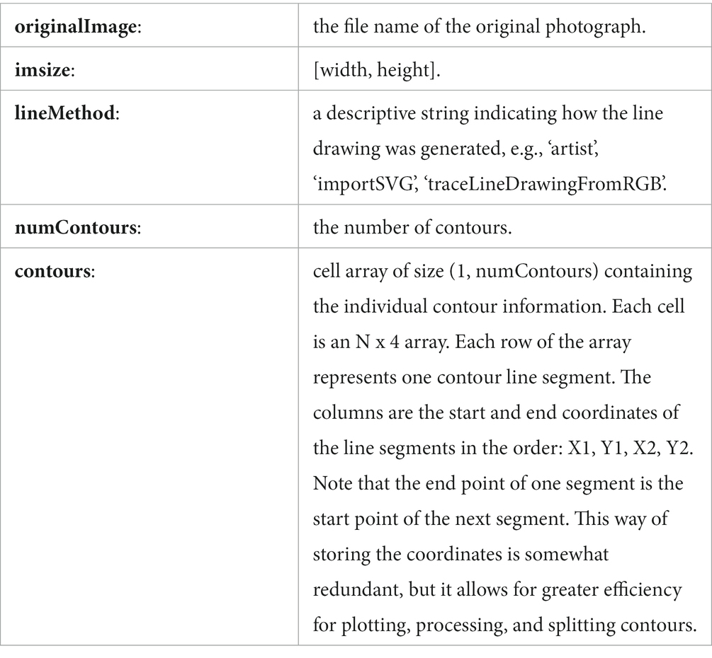
Both methods result in vectorized line drawings that are represented as a set of contours (Figure 1). Each contour consists of a list of successive, connected straight line segments. The information is contained in a vecLD struct with the following fields:

FIGURE 1

Figure 1. Color photograph of a forest (left), extracted contours (middle), contours superimposed on the original image (right).

More fields are added to the struct as image properties are computed. Vectorized line drawings can be plotted into a figure window using the drawLinedrawing function. They can be rendered into a binary image using the renderLinedrawing function.

Measuring contour properties

Analysis of properties of individual contours and contour segments follows the intuitive definitions outlined below.

Orientation of individual contours is computed as:

$ori=\arctan \left(\frac{Y2-Y1}{X2-X1}\right)$

where orientations are measured in degrees in the counterclockwise direction, starting from 0^° at horizontal all the way to 360^° back at horizontal. Orientations are stored in a direction-specific way so that 180^° is not considered the same as 0^°. This coding is important for computing curvature and junction angles correctly.

When computing histograms of orientation, however, orientation angles are computed modulo 180 degrees. Orientation histograms are weighted by the number of pixels (length) of a particular line segment. By default, eight histograms are computed with bin centers at 0, 22.5, 45, 67.5, 90, 112.5, 135, and 157.5 degrees.

Functions: computeOrientation , getOrientationStats

The length of contour segments is computed as the Euclidean distance between the start and end points:

$length=\sqrt{{\left(X2-X1\right)}^2+{\left(Y2-Y1\right)}^2}$

The length of an entire contour is the sum of the lengths of the individual contour segments. Contour histograms are computed with bins equally spaced on a logarithmic scale within the bounds of 2 pixels and (width + height). For instance, an eight-bin histogram (the default) for images of size 800 × 600 pixels has bin centers located at 3.4, 8.5, 19.5, 43.2, 94.2, 204.2, 441.5, and 953.1 pixels.

Functions: computeLength , getLengthStats

Mathematically, curvature is defined as the change in angle per unit length. In calculus, the change of angle is given by the second derivative. For the piecewise straight line segments in our implementation, we compute the curvature for each line segment as the amount of change in orientation from this to the next line segment, divided by the length of the segment:

$curvatur{e}_i=\frac{\mathrm{mod}\left(or{i}_{i+1}-or{i}_i\mathrm{,}180\right)}{lengt{h}_i}$

For the last segment of a contour, we use the angle difference with the previous instead of the next segment. Histograms of contour curvature are computed with bins equally spaced on a logarithmic scale between 0 degrees / pixel (straight line; no curvature) and 90 degrees / pixel (a minimal line of 2 pixels length making a sharp 180-degree turn). For a default eight-bin histogram, bins are centered at 0.33, 1.33, 3.09, 6.20, 11.65, 21.23, 38.06, and 67.64 degrees per pixel.

Functions: computeCurvature , getCurvatureStats

Contour junctions are detected at the intersections between contours. The intersections are computed algebraically from the coordinates of all contour segments. Intersections of contour segments within a contour are not considered. Junctions are still detected when contours do not meet exactly. This function is controlled by two parameters, a relative epsilon (RE) and an absolute epsilon (AE). The relative epsilon controls the allowable gap between the end point of a contour segment and the hypothetical junction location as the fraction of the length of the contour segment. The absolute epsilon determines the maximum allowable gap in pixels. The minimum between the two gap measures is used as a threshold value for detecting junctions. Hand tuning of the parameters resulted in values of AE = 1 pixel and RE = 0.3. These two parameters can be set as optional arguments of the detectJunctions function.

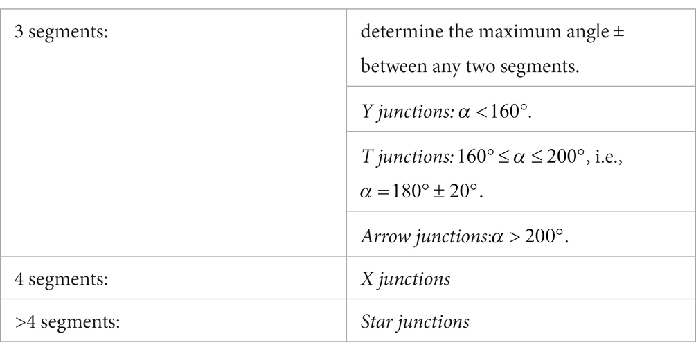
Contour segments participating in junctions are algorithmically severed into two new segments at the junction locations whenever junctions are detected far enough away from the end points. The angles between all segments participating in a junction are measured as the difference in (directed) orientation angle between adjacent segments. Inspired by previous literature on contour junctions (Biederman, 1987), junction types are classified according to how many contour segments participate in the junction and according to their angles as follows:

Junctions between two contour segments are sometimes described as L junctions. Here, we do not consider L junctions as they would occur at every location where one contour segment ends and the next begins, making them too numerous to be useful.

Integer counts of the number of junctions of each count are collected in junction histograms, which can optionally be normalized by the total number of pixels in a vectorized line drawing. The minimum angles between any of the contour segments, which are bounded between 0 and 120 degrees, are also counted as “Junction Angles” in a histogram with bin centers at 7.5, 22.5, 37.5, 52.5, 67.5, 82.5, 97.5, and 112.5 degrees.

Functions: computeJunctions , getJunctionStats , detectJunctions

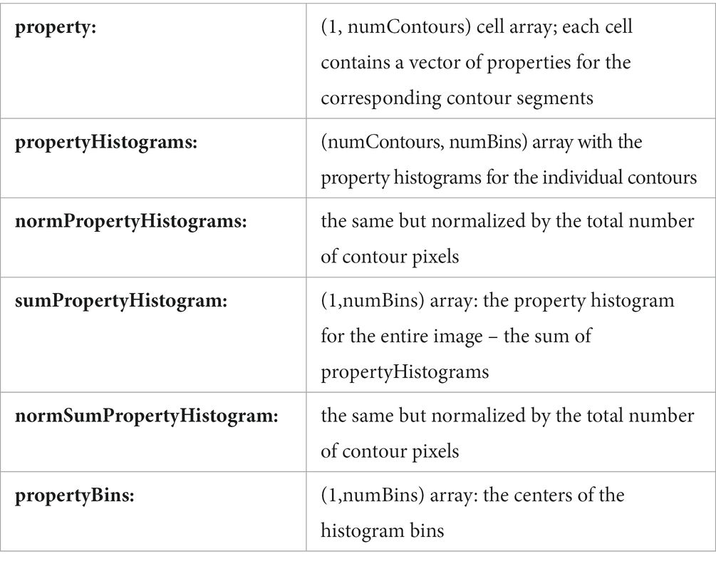
For each contour property, the following fields are added to the vecLD struct:

To visualize the contour properties, use the drawLinedrawingProperty function (Figure 2). The first argument to the function is a vecLD struct, the second a string denoting the contour property. The function draws the color drawing into the current figure window. Use drawAllProperties to visualize all contour properties for a given vecLD struct, either using subplots or in separate figure windows. The renderLinedrawingProperty function draws the contour properties into an image instead of a figure.

FIGURE 2

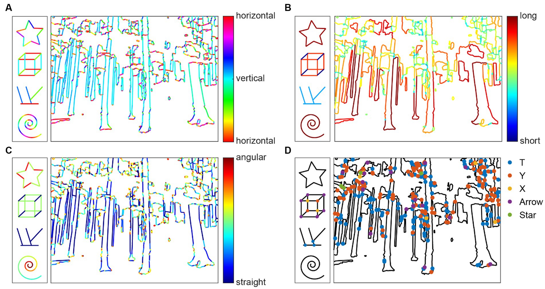
Figure 2. Visualization of contour properties Orientation (A), Contour Length (B), Curvature (C), and Contour Junctions (D) for the example images as well as four simple test shapes.

We have used these contour properties previously to explain behavior (Walther and Shen, 2014; Wilder et al., 2018) and neural mechanisms of scene categorization (Choo and Walther, 2016). We have also related statistics of these properties to the emotional content of scenes and generated artificial images with specific property combinations to elicit emotional responses (Damiano et al., 2021a), as well as to esthetic pleasure (Farzanfar and Walther, 2023).

Medial axis-based properties

Blum (1967) was probably the first to introduce medial axis-based representations and the method for producing them using a grassfire analogy. Imagine a shape cut out of a piece of paper set on fire around its border, where the fire front moves toward the center of the shape at a constant pace. Skeletal points are formed at the locations where the fire fronts collide. In other words, we can look at the Medial Axis Transform (MAT) as a method for applying the grassfire process to disclose its quench sites and associated radius values (Feldman and Singh, 2006). The MAT provides a complete visual representation of shapes, as it is applicable to all bounded shapes as well as the areas outside of closed shapes. Humans have been shown to rely on the shape skeleton defined by the MAT when they attend to objects (Firestone and Scholl, 2014), represent shapes in memory (Ayzenberg and Lourenco, 2019), or judge the esthetic appeal of shapes (Sun and Firestone, 2022).

In this toolbox, we compute measures of the relationships between contours using the medial axis transform. Visually, the medial axis transform is made up of a number of branches that come together at branch points to create a shape skeleton. A group of contiguous regular points from the skeleton that are located between two junction points, two end points, or an end point and a junction point are known as skeletal branches. The behavior of the average outward flux (AOF) of the gradient of the Euclidean distance function to the boundary of a 2D object through a shrinking disk can be used to identify skeletal points that lie on skeletal branches and identify the types of those three classes of points, as demonstrated by Rezanejad (2020). We go over this calculation in the following.

Imagine that the distance transform $D_{\Omega }$ of a shape Ω is a signed distance function that indicates the closest distance of a given point $p$ to the shape’s boundary $\partial \Omega$ (Figure 3A). Formally, we can imagine a positive sign for the distance value when $p$ is inside the shape Ω and a negative sign when $p$ is outside of the shape Ω. We can then define the distance function gradient vector for point $p$ as ${\dot{q}}_{\Omega }\left(p\right)$ as the unit vector that connects point $p$ to its closest boundary point. One of the ways to identify skeletal points is to investigate the distance function gradient vector which is multivalued at the skeletal points. To do this investigation, we use a measure called AOF (Average Outward Flux). To compute AOF, we compute the outward flux of $\dot{q}$ through shrinking circular neighborhoods all over the image:

$AOF=\frac{{{\displaystyle \int }}_{\partial R}〈\dot{q}\mathrm{,}N\partial S〉}{{{\displaystyle \int }}_{\partial R}\partial S}$

where $\partial R$ is the boundary of the shrinking circular neighborhood and $N$ is the normal to the boundary (Figure 3B). By analyzing the behavior of AOF, we can classify each point into a medial axis or non-medial axis point. In particular, any points that are not on the skeleton have a limiting AOF value of zero, so the medial axis is the set of points where their AOF values are non-zero (Figure 3C). The AOF value has a sinusoidal relationship with the object angle (the mid-angle between spoke vectors that connect a skeletal point to the closest boundary points). In the discrete space, we threshold the AOF based on a particular value, which means that we keep skeletal points that have object angles above a certain degree. The object angle can be provided as an optional parameter for the computeMAT function, with a default value of 28 degrees (Rezanejad, 2020). We compute three local relational properties based on the medial axis transform.

FIGURE 3

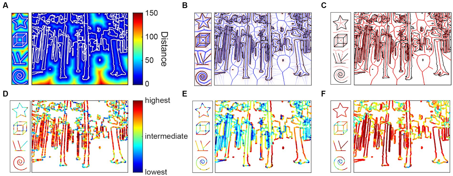
Figure 3. Medial axis properties. (A) Distance function from the contours (white); (B) Average outward flux (blue) from the contours (black); (C) Medial axes (red) between the contours; (D) Parallelism scores mapped onto the contours; (E) Separation scores; (F) Mirror symmetry scores.

Parallelism is computed as the local ribbon symmetry by computing the first derivative of the radial distance function along the medial axis. A small first derivative (small change) indicates that the contours on either side of the medial axis are locally parallel to the medial axis and, thereby, to each other (Figure 3D).

Separation is computed as the absolute value of the radial distance function. Separation is related to the Gestalt grouping rule of proximity (Figure 3E).

Mirror symmetry is generally understood to be the symmetry generated by reflection over a straight axis. Reflections over bent axes are not perceived as mirror symmetric. We therefore compute the curvature of the medial axis as a measure of local mirror symmetry. The straighter the medial axis is, the stronger is local mirror symmetry (Figure 3F).

These properties are initially computed on the medial axis and then projected back onto the contours of the line drawing and normalized to [0,1]. Note that not all contour pixels may receive a valid MAT property, since the projection from the medial axis back to the contour pixels is not a surjective function. As mentioned above, we apply a small threshold on the AOF values in discrete pixel space to compute a medial axis that is thin, smooth and does not cover the entire area of the interior shape. While the analytical formulation of the medial axis is a one-to-many mapping from skeletal points to the boundary that ensures that all the boundary points are reconstructable in the discrete space, we may lose a small portion of the boundary points that will not be associated with the skeletal points.

Functions: computeMAT , computeMATproperty , mapMATtoContour , computeAllMATproperties

To compute statistics over the MAT properties along the contours, the contours are mapped to the vectorized line drawing. Histograms with equally spaced bins (default: 8 bins) to cover the interval [0,1] are computed over all contour pixels with valid MAT properties.

Functions: MATpropertiesToContours , getMATpropertyStats , computeAllMATfromVecLD

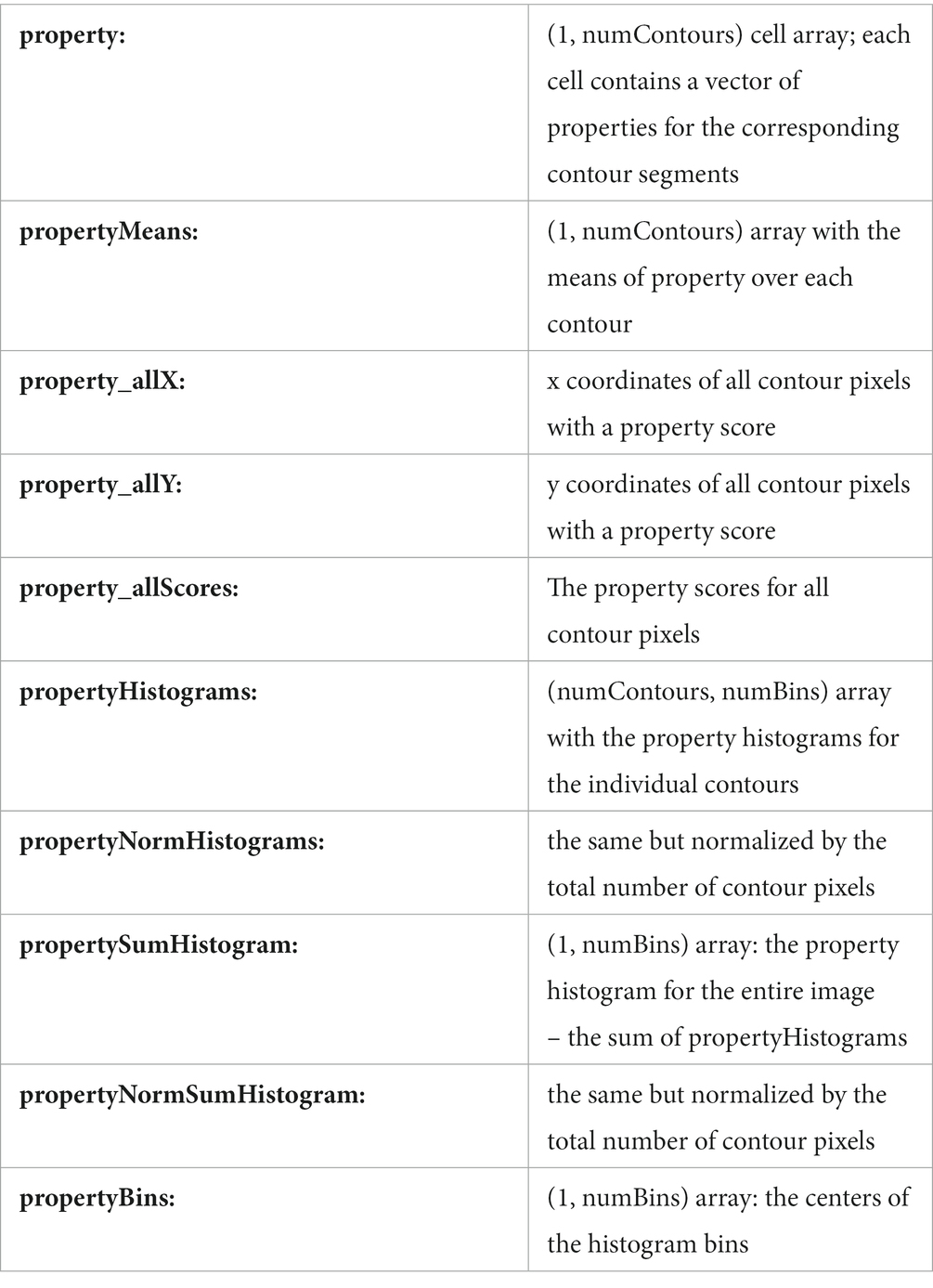
Similar to the contour properties, the following fields are added to the vecLD struct for each MAT property:

MAT properties are easily visualized in a figure using drawMATproperty or drawn into an image using renderMATproperty .

The histograms for all image properties can be written into a table for a set of images for further statistical analysis. The function allLDHistogramsToTable generates such a table, which can then be used with Matlab’s statistical functions or be written to a CSV file for further processing in R or other analysis software.

We have used these functions to investigate the role of MAT-based features for computer vision (Rezanejad et al., 2019, 2023), eye movements (Damiano et al., 2019), neural representations of symmetry (Wilder et al., 2022), to investigate esthetic appeal (Damiano et al., 2021b; Farzanfar and Walther, 2023) and image memorability (Han et al., 2023).

Splitting functions

Splitting the contours in a line drawing into two halves based on some statistical property allows for the empirical testing of the causal involvement of that property in some perceptual or cognitive function. We provide functions for separating contours into two drawings by different criteria:

splitLDbyProperties : allows for the splitting according to one image property or a combination of image properties. The function also contains an option to generate a random split of the contours. We have used this function to split images by their MAT properties for behavioral and fMRI experiments as well as for computer vision analyses (Rezanejad et al., 2019, 2023; Wilder et al., 2022).

splitLDbyHistogramWeights : allows for splitting the contours according to more fine-grained weights for the individual feature histograms.

splitLDbyStatsModel : splits the contours by the output of a statistical model, trained with the contour and MAT properties as its features. This function has been used to split contours according to predicted esthetic appeal (Farzanfar and Walther, 2023) or according to predicted memorability (Han et al., 2023).

splitLDmiddleSegmentsVsJunctions : Splits the contours into pieces near the contour junctions and middle segments. This method was used to investigate the role junctions for scene categorization (Wilder et al., 2018).

For an input vecLD struct, these functions generate two new, disjoint vecLD structs, each with approximately half of the pixels (Figure 4). Contours that cannot be uniquely assigned to one or the other drawing are omitted from both.

FIGURE 4

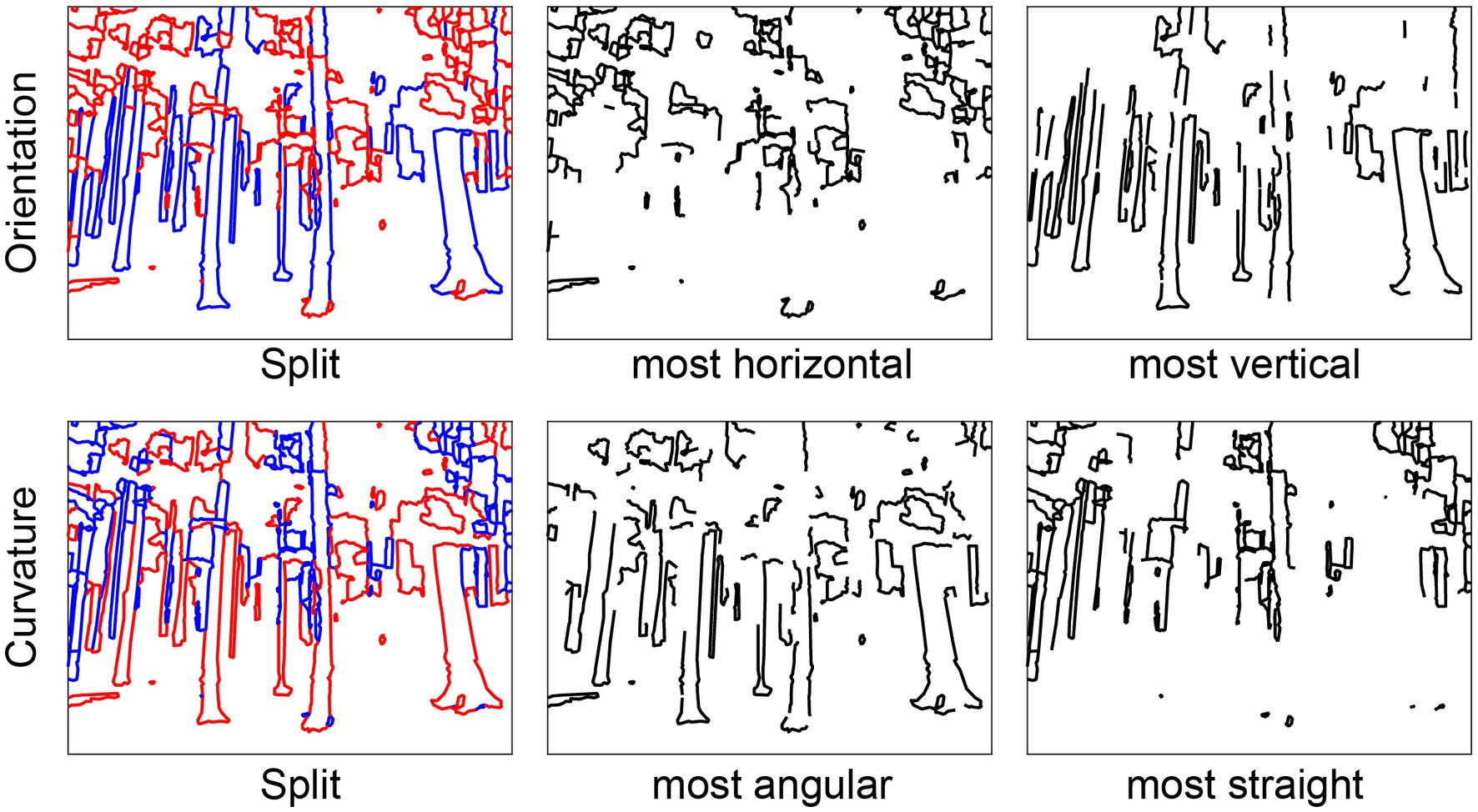
Figure 4. Splitting functions. Left column: Line drawings split into top (red) and bottom (blue) halves according to Orientation (“top” = horizontal, “bottom” = vertical) and Curvature (“top” = angular, “bottom” = straight). Middle column: drawings with only the top halves. Right column: drawings with only the bottom halves.

Other image transformations

We include some other specific manipulations of the line drawing images that have proven useful in manipulating images (Figure 5). The function rotateLinedrawing rotates the coordinates of all contours in the input vecLD structure by a given angle, and applyCircularAperture clips the contours to a circular aperture. In combination, these functions can be used to generate randomly rotated line drawings (Choo and Walther, 2016).

FIGURE 5

Figure 5. Image transformation functions. (A) Applying circular aperture; (B) rotating the image by an arbitrary angel (here: 63°); (C) randomly shifting contours.

Randomly shifting individual contours within the image bounding box destroys the distribution of contour junctions while keeping the statistics of orientation, length, and curvature constant (Walther and Shen, 2014; Choo and Walther, 2016). This functionality is provided by randomlyShiftContours .

Datasets

We provide five data sets already processed as vecLD structs:

• A set of 475 images of six scene categories (beaches, cities, forests, highways, mountains, and offices). The line drawings were created by trained artists at the Lotus Hill Institute in Fudan, People’s Republic of China.

• Line drawings of the 1,182 images in the International Affective Picture System (IAPS) (Lang et al., 2008), also created at the Lotus Hill Institute.

• Hand-traced drawings of 260 objects from (Snodgrass and Vanderwart, 1980).

• A set of 200 architectural scenes published in (Vartanian et al., 2013), traced automatically using traceLineDrawingFromRGB .

• Line drawings of the 900 images in the Open Affective Standardized Image Set (OASIS) (Kurdi et al., 2017).

We plan to add more datasets in the near future.

Conclusion

A major obstacle for research on the role of mid-level visual features in the perception of complex, real-world scenes has been the capability to measure and selectively manipulate these features in scenes. We offer the Mid-level Vision Toolbox to the research community as way to overcome this obstacle and enable future research on this topic. We include functionality for assessing a variety of low- and mid-level features based on the geometry of contours, as well as functions for generating contour line drawings from RGB images and functions for manipulating such drawings.

The easily accessible data structures and function interfaces of MLV Toolbox allow for future expansions of its functionality. For instance, symmetry relationships, limited to the nearest contours in the current implementation, could be expanded to include symmetries across larger scales. Another expansion could be the detection of another important grouping cue, closure of contours. Figure-ground segmentation cues, such as border ownership could be included in the future as well. Our group will continue to work on expanding the functionality of the toolbox, and we also invite contributions from other researchers.

Computational models of visual perception in humans and non-human primates have progressed rapidly in recent years, thanks to the advent of convolutional neural networks (Krizhevsky et al., 2012). Convolutional Neural Networks have been shown to correlate well with biological vision systems (e.g., Cadieu et al., 2014; Khaligh-Razavi and Kriegeskorte, 2014; Yamins et al., 2014; Güçlü and van Gerven, 2015), and they are getting closer to replicating the functionality of biological systems all the time (Schrimpf et al., 2020). Why, then, should we care about hand-coded algorithms for detecting mid-level features as in the MLV Toolbox? Despite these models’ increasing ability to match biological vision, the mechanisms underlying their impressive performance are barely any clearer than those underlying biological vision. We need to probe these deep neural networks empirically to better understand the mechanisms underlying the function (Bowers et al., 2022).

A century of empirical research as well as existing practice in design and architecture have unequivocally demonstrated the importance of Gestalt grouping rules for human perception (Wagemans et al., 2012) as well as esthetic appreciation (Arnheim, 1965; Leder et al., 2004; Chatterjee, 2022). To what extent convolutional neural networks learn to represent these grouping rules is an open question. We know from work with random dot patterns that the human brain represents symmetry relationships in fairly high-level areas, such as the object-sensitive lateral occipital complex (Bona et al., 2014, 2015). We are only starting to learn how the brain represents Gestalt grouping rules for perceiving complex scenes (Wilder et al., 2022).

We here provide a set of computational tools that will enable studies of the mid-level representations that arise in both biological and artificial vision systems. Although the specific computations used here to measure mid-level visual properties are unlikely to be an accurate reflection of the neural mechanisms in the human visual system, we nevertheless believe that measuring and manipulating mid-level visual cues in complex scenes will be instrumental in furthering our understanding of visual perception.

Data availability statement

The datasets presented in this study can be found at: http://mlvtoolbox.org.

Author contributions

DW and MR contributed to the algorithms and their implementation in the toolbox. DF and SH tested the code and provided suggestions and feedback for features and improvements. DW wrote the first draft of the manuscript. MR and DF wrote sections of the manuscript. All authors contributed to the article and approved the submitted version.

Funding

This work was supported by an NSERC Discovery grant (RGPIN-2020-04097) and an XSeed grant from the Faculty of Applied Science and Engineering and the Faculty of Arts and Science of the University of Toronto to DW, an Alexander Graham Bell Canada Graduate Scholarship from NSERC to DF, a Connaught International Scholarship to SH, and a Faculty of Arts and Science Postdoctoral Fellowship to MR.

Conflict of interest

The authors declare that the research was conducted in the absence of any commercial or financial relationships that could be construed as a potential conflict of interest.

Publisher’s note

All claims expressed in this article are solely those of the authors and do not necessarily represent those of their affiliated organizations, or those of the publisher, the editors and the reviewers. Any product that may be evaluated in this article, or claim that may be made by its manufacturer, is not guaranteed or endorsed by the publisher.

Footnotes

1. ^ http://mlvtoolbox.org

2. ^ https://github.com/pdollar/edges

3. ^ https://www.peterkovesi.com/matlabfns/#edgelink

References

Arnheim, R. (1965). Art and visual perception: A psychology of the creative eye. Berkeley, California: Univ of California Press.

Google Scholar

Ayzenberg, V., Kamps, F. S., Dilks, D. D., and Lourenco, S. F. (2022). Skeletal representations of shape in the human visual cortex. Neuropsychologia 164:108092. doi: 10.1016/j.neuropsychologia.2021.108092

PubMed Abstract | CrossRef Full Text | Google Scholar

Ayzenberg, V., and Lourenco, S. F. (2019). Skeletal descriptions of shape provide unique perceptual information for object recognition. Sci. Rep. 9:9359. doi: 10.1038/s41598-019-45268-y

PubMed Abstract | CrossRef Full Text | Google Scholar

Biederman, I. (1987). Recognition-by-components: a theory of human image understanding. Psychol. Rev. 94, 115–147. doi: 10.1037/0033-295X.94.2.115

PubMed Abstract | CrossRef Full Text | Google Scholar

Blum, H. (1967). A transformation for extracting new descriptions of shape. Cambridge, Massachusetts: MIT Press.

Google Scholar

Bona, S., Cattaneo, Z., and Silvanto, J. (2015). The causal role of the occipital face area (OFA) and lateral occipital (LO) cortex in symmetry perception. J. Neurosci. 35, 731–738. doi: 10.1523/JNEUROSCI.3733-14.2015

PubMed Abstract | CrossRef Full Text | Google Scholar

Bona, S., Herbert, A., Toneatto, C., Silvanto, J., and Cattaneo, Z. (2014). The causal role of the lateral occipital complex in visual mirror symmetry detection and grouping: an fMRI-guided TMS study. Cortex 51, 46–55. doi: 10.1016/j.cortex.2013.11.004

PubMed Abstract | CrossRef Full Text | Google Scholar

Bowers, J. S., Malhotra, G., Duimovic, M., Montero, M. L., Tsvetkov, C., Biscione, V., et al. (2022). Deep problems with neural network models of human vision. Behav. Brain Sci. 1, 1–74. doi: 10.1017/S0140525X22002813

CrossRef Full Text | Google Scholar

Cadieu, C. F., Hong, H., Yamins, D. L., Pinto, N., Ardila, D., Solomon, E. A., et al. (2014). Deep neural networks rival the representation of primate IT cortex for core visual object recognition. PLoS Comput. Biol. 10:e1003963. doi: 10.1371/journal.pcbi.1003963

PubMed Abstract | CrossRef Full Text | Google Scholar

Chatterjee, A. (2022). “An early framework for a cognitive neuroscience of visual aesthetics” in Brain, beauty, & art. eds. A. Chatterjee and E. R. Cardillo (Essays Bringing Neuroaesthetics in Focus, New York, NY: Oxford University Press)

Google Scholar

Choo, H., and Walther, D. B. (2016). Contour junctions underlie neural representations of scene categories in high-level human visual cortex. NeuroImage 135, 32–44. doi: 10.1016/j.neuroimage.2016.04.021

PubMed Abstract | CrossRef Full Text | Google Scholar

Damiano, C., Walther, D. B., and Cunningham, W. A. (2021a). Contour features predict valence and threat judgements in scenes. Sci. Rep. 11, 1–12. doi: 10.1038/s41598-021-99044-y

CrossRef Full Text | Google Scholar

Damiano, C., Wilder, J., and Walther, D. B. (2019). Mid-level feature contributions to category-specific gaze guidance. Atten. Percept. Psychophys. 81, 35–46. doi: 10.3758/s13414-018-1594-8

PubMed Abstract | CrossRef Full Text | Google Scholar

Damiano, C., Wilder, J., Zhou, E. Y., Walther, D. B., and Wagemans, J. (2021b). The role of local and global symmetry in pleasure, interest, and complexity judgments of natural scenes. Psychol. Aesthet. Creat. Arts 17, 322–337. doi: 10.1037/aca0000398

CrossRef Full Text | Google Scholar

De Winter, J., and Wagemans, J. (2006). Segmentation of object outlines into parts: a large-scale integrative study. Cognition 99, 275–325. doi: 10.1016/j.cognition.2005.03.004

PubMed Abstract | CrossRef Full Text | Google Scholar

Desolneux, A., Moisan, L., and Morel, J.-M. (2004). “Gestalt theory and computer vision,” in Seeing, thinking and knowing: Meaning and self-organisation in visual cognition and thought. Dordrecht: Springer Netherlands, 71–101.

Google Scholar

Desolneux, A., Moisan, L., and Morel, J.-M., (2007). From gestalt theory to image analysis: A probabilistic approach. Springer Science & Business Media, New York, NY

Google Scholar

Dollár, P., and Zitnick, C. L., (2013). Structured forests for fast edge detection, in: Proceedings of the IEEE International Conference on Computer Vision. pp. 1841–1848.

Google Scholar

Dollár, P., and Zitnick, C. L. (2014). Fast edge detection using structured forests. IEEE Trans. Pattern Anal. Mach. Intell. 37, 1558–1570. doi: 10.1109/TPAMI.2014.2377715

CrossRef Full Text | Google Scholar

Elder, J. H., and Goldberg, R. M. (2002). Ecological statistics of gestalt laws for the perceptual organization of contours. J. Vis. 2, 5–353. doi: 10.1167/2.4.5

PubMed Abstract | CrossRef Full Text | Google Scholar

Elder, J., and Zucker, S. (1993). The effect of contour closure on the rapid discrimination of two-dimensional shapes. Vis. Res. 33, 981–991. doi: 10.1016/0042-6989(93)90080-G

PubMed Abstract | CrossRef Full Text | Google Scholar

Epstein, R., DeYoe, E. A., Press, D. Z., Rosen, A. C., and Kanwisher, N. (2001). Neuropsychological evidence for a topographical learning mechanism in parahippocampal cortex. Cogn. Neuropsychol. 18, 481–508. doi: 10.1080/02643290125929

PubMed Abstract | CrossRef Full Text | Google Scholar

Epstein, R., and Kanwisher, N. (1998). A cortical representation of the local visual environment. Nature 392, 598–601. doi: 10.1038/33402

CrossRef Full Text | Google Scholar

Farzanfar, D., and Walther, D. B. (2023). Changing What You Like: Modifying Contour Properties Shifts Aesthetic Valuations of Scenes. Psychol. Sci. doi: 10.1177/09567976231190546. [Epub ahead of print].

CrossRef Full Text | Google Scholar

Feldman, J., and Singh, M. (2005). Information along contours and object boundaries. Psychol. Rev. 112, 243–252. doi: 10.1037/0033-295X.112.1.243

PubMed Abstract | CrossRef Full Text | Google Scholar

Feldman, J., and Singh, M. (2006). Bayesian estimation of the shape skeleton. Proc. Natl. Acad. Sci. 103, 18014–18019. doi: 10.1073/pnas.0608811103

PubMed Abstract | CrossRef Full Text | Google Scholar

Field, D. J., Hayes, A., and Hess, R. F. (1993). Contour integration by the human visual system: evidence for a local “association field”. Vis. Res. 33, 173–193. doi: 10.1016/0042-6989(93)90156-Q

PubMed Abstract | CrossRef Full Text | Google Scholar

Firestone, C., and Scholl, B. J. (2014). “Please tap the shape, anywhere you like” shape skeletons in human vision revealed by an exceedingly simple measure. Psychol. Sci. 25, 377–386. doi: 10.1177/0956797613507584

PubMed Abstract | CrossRef Full Text | Google Scholar

Gallant, J. L., Connor, C. E., Rakshit, S., Lewis, J. W., and Van Essen, D. C. (1996). Neural responses to polar, hyperbolic, and Cartesian gratings in area V4 of the macaque monkey. J. Neurophysiol. 76, 2718–2739. doi: 10.1152/jn.1996.76.4.2718

PubMed Abstract | CrossRef Full Text | Google Scholar

Geisler, W. S., Perry, J. S., Super, B. J., and Gallogly, D. P. (2001). Edge co-occurrence in natural images predicts contour grouping performance. Vis. Res. 41, 711–724. doi: 10.1016/S0042-6989(00)00277-7

PubMed Abstract | CrossRef Full Text | Google Scholar

Güçlü, U., and van Gerven, M. A. (2015). Deep neural networks reveal a gradient in the complexity of neural representations across the ventral stream. J. Neurosci. 35, 10005–10014. doi: 10.1523/JNEUROSCI.5023-14.2015

PubMed Abstract | CrossRef Full Text | Google Scholar

Han, S., Rezanejad, M., and Walther, D. B. (2023). Making memorability of scenes better or worse by manipulating their contour properties. J. Vis. 23:5494. doi: 10.1167/jov.23.9.5494

CrossRef Full Text | Google Scholar

Hubel, D. H., and Wiesel, T. N. (1962). Receptive fields, binocular interaction and functional architecture in the cat’s visual cortex. J. Physiol. 160, 106–154. doi: 10.1113/jphysiol.1962.sp006837

PubMed Abstract | CrossRef Full Text | Google Scholar

Khaligh-Razavi, S.-M., and Kriegeskorte, N. (2014). Deep supervised, but not unsupervised, models may explain IT cortical representation. PLoS Comput. Biol. 10:e1003915. doi: 10.1371/journal.pcbi.1003915

PubMed Abstract | CrossRef Full Text | Google Scholar

Koffka, K. , (1935). Principles of gestalt psychology. Harcourt Brace and Company, New York, NY.

Google Scholar

Krizhevsky, A., Sutskever, I., and Hinton, G. E. (2012). “ImageNet classification with deep convolutional neural networks” in Advances in neural information processing systems. eds. F. Pereira, C. J. Burges, L. Bottou, and K. Q. Weinberger (United States: Curran Associates, Inc)

Google Scholar

Kubovy, M. (1994). The perceptual organization of dot lattices. Psychon B Rev 1, 182–190. doi: 10.3758/bf03200772

PubMed Abstract | CrossRef Full Text | Google Scholar

Kurdi, B., Lozano, S., and Banaji, M. R. (2017). Introducing the open affective standardized image set (OASIS). Behav. Res. Methods 49, 457–470. doi: 10.3758/s13428-016-0715-3

PubMed Abstract | CrossRef Full Text | Google Scholar

Lang, P. J., Bradley, M. M., and Cuthbert, B. N. (2008). International affective picture system (IAPS): Affective ratings of pictures and instruction manual. University of Florida, Gainsville, FL.

Google Scholar

Leder, H., Belke, B., Oeberst, A., and Augustin, D. (2004). A model of aesthetic appreciation and aesthetic judgments. Brit J Psychol 95, 489–508. doi: 10.1348/0007126042369811

CrossRef Full Text | Google Scholar

Lowe, D. G. (1987). Three-dimensional object recognition from single two-dimensional images. Artif. Intell. 31, 355–395. doi: 10.1016/0004-3702(87)90070-1

CrossRef Full Text | Google Scholar

Lowe, D. (2012). Perceptual organization and visual recognition. Springer Science & Business Media. New York

Google Scholar

Machilsen, B., Pauwels, M., and Wagemans, J. (2009). The role of vertical mirror symmetry in visual shape detection. J. Vis. 9:11. doi: 10.1167/9.12.11

CrossRef Full Text | Google Scholar

Malcolm, G. L., Groen, I. I. A., and Baker, C. I. (2016). Making sense of real-world scenes. Trends Cogn. Sci. 20, 843–856. doi: 10.1016/j.tics.2016.09.003

PubMed Abstract | CrossRef Full Text | Google Scholar

Marr, D. , (1982). Vision: A computational investigation into the human representation and processing of visual information.

Google Scholar

Marr, D., and Nishihara, H. K. (1978). Representation and recognition of the spatial organization of three-diemnsional shapes. Proccedings of the Royal Soc London B. 200, 269–294. doi: 10.1098/rspb.1978.0020

CrossRef Full Text | Google Scholar

Michaelsen, E., and Meidow, J. (2019). Hierarchical perceptual grouping for object recognition Springer, New York.

Google Scholar

Norcia, A. M., Candy, T. R., Pettet, M. W., Vildavski, V. Y., and Tyler, C. W. (2002). Temporal dynamics of the human response to symmetry. J. Vis. 2, 1–139. doi: 10.1167/2.2.1

PubMed Abstract | CrossRef Full Text | Google Scholar

Olshausen, B. A., and Field, D. J. (1996). Emergence of simple-cell receptive field properties by learning a sparse code for natural images. Nature 381, 607–609. doi: 10.1038/381607a0

PubMed Abstract | CrossRef Full Text | Google Scholar

Pasupathy, A., and Connor, C. E. (2002). Population coding of shape in area V4. Nat. Neurosci. 5, 1332–1338. doi: 10.1038/972

CrossRef Full Text | Google Scholar

Peirce, J. W. (2015). Understanding mid-level representations in visual processing. J. Vis. 15:5. doi: 10.1167/15.7.5

PubMed Abstract | CrossRef Full Text | Google Scholar

Peterhans, E., and von der Heydt, R. (1989). Mechanisms of contour perception in monkey visual cortex. II. Contours bridging gaps. J. Neurosci. 9, 1749–1763. doi: 10.1523/JNEUROSCI.09-05-01749.1989

PubMed Abstract | CrossRef Full Text | Google Scholar

Pizlo, Z., Li, Y., and Sawada, T., (2014). Making a machine that sees like us. Oxford University Press, USA.

Google Scholar

Rezanejad, M. , (2020). Medial measures for recognition, mapping and categorization, McGill University. Canada

Google Scholar

Rezanejad, M., Downs, G., Wilder, J., Walther, D. B., Jepson, A., Dickinson, S., et al. (2019). Scene categorization from contours: medial Axis based salience measures. Proc. IEEE Conf. Comput. Vis. Pattern Recognit., 4116–4124.

Google Scholar

Rezanejad, M., Wilder, J., Walther, D. B., Jepson, A., Dickinson, S., and Siddiqi, K. (2023). Shape Based Measures Improve Scene Categorization. under review. IEEE Trans. Pattern Anal. Mach. Intell.

Google Scholar

Sasaki, Y. (2007). Processing local signals into global patterns. Curr. Opin. Neurobiol. 17, 132–139. doi: 10.1016/j.conb.2007.03.003

CrossRef Full Text | Google Scholar

Schrimpf, M., Kubilius, J., Lee, M. J., Murty, N. A. R., Ajemian, R., and DiCarlo, J. J. (2020). Integrative benchmarking to advance Neurally mechanistic models of human intelligence. Neuron 108, 413–423. doi: 10.1016/j.neuron.2020.07.040

PubMed Abstract | CrossRef Full Text | Google Scholar

Snodgrass, J. G., and Vanderwart, M. (1980). A standardized set of 260 pictures: norms for name agreement, image agreement, familiarity, and visual complexity. J. Exp. Psychol. 6, 174–215. doi: 10.1037/0278-7393.6.2.174

CrossRef Full Text | Google Scholar

Sun, Z., and Firestone, C. (2022). Beautiful on the inside: aesthetic preferences and the skeletal complexity of shapes. Perception 51, 904–918. doi: 10.1177/03010066221124872

PubMed Abstract | CrossRef Full Text | Google Scholar

Vartanian, O., Navarrete, G., Chatterjee, A., Fich, L. B., Leder, H., Modroño, C., et al. (2013). Impact of contour on aesthetic judgments and approach-avoidance decisions in architecture. Proc National Acad Sci 110, 10446–10453. doi: 10.1073/pnas.1301227110

PubMed Abstract | CrossRef Full Text | Google Scholar

Vinje, W. E., and Gallant, J. L. (2000). Sparse coding and decorrelation in primary visual cortex during natural vision. Science 287, 1273–1276. doi: 10.1126/science.287.5456.1273

PubMed Abstract | CrossRef Full Text | Google Scholar

Wagemans, J. (1993). Skewed symmetry: a nonaccidental property used to perceive visual forms. J. Exp. Psychol. Hum. Percept. Perform. 19, 364–380. doi: 10.1037/0096-1523.19.2.364

PubMed Abstract | CrossRef Full Text | Google Scholar

Wagemans, J. (1997). Characteristics and models of human symmetry detection. Trends Cogn. Sci. 1, 346–352. doi: 10.1016/s1364-6613(97)01105-4

CrossRef Full Text | Google Scholar

Wagemans, J., Elder, J. H., Kubovy, M., Palmer, S. E., Peterson, M. A., Singh, M., et al. (2012). A century of gestalt psychology in visual perception: I. perceptual grouping and figure–ground organization. Psychol. Bull. 138, 1172–1217. doi: 10.1037/a0029333

PubMed Abstract | CrossRef Full Text | Google Scholar

Walther, D. B., and Shen, D. (2014). Nonaccidental properties underlie human categorization of complex natural scenes. Psychol. Sci. 25, 851–860. doi: 10.1177/0956797613512662

PubMed Abstract | CrossRef Full Text | Google Scholar

Wertheimer, M. (1922). Untersuchungen zur Lehre von der Gestalt, I: Prinzipielle Bemerkungen [Investigations in Gestalt theory: I. The general theoretical situation]. Psychol. Forsch. 1, 47–58. doi: 10.1007/BF00410385

CrossRef Full Text | Google Scholar

Wilder, J., Dickinson, S., Jepson, A., and Walther, D. B. (2018). Spatial relationships between contours impact rapid scene classification. J. Vis. 18:1. doi: 10.1167/18.8.1

PubMed Abstract | CrossRef Full Text | Google Scholar

Wilder, J., Rezanejad, M., Dickinson, S., Siddiqi, K., Jepson, A., and Walther, D. B. (2022). Neural correlates of local parallelism during naturalistic vision. PLoS One 17:e0260266. doi: 10.1371/journal.pone.0260266

PubMed Abstract | CrossRef Full Text | Google Scholar

Yamins, D. L., Hong, H., Cadieu, C. F., Solomon, E. A., Seibert, D., and DiCarlo, J. J. (2014). Performance-optimized hierarchical models predict neural responses in higher visual cortex. Proc. Natl. Acad. Sci. 111, 8619–8624. doi: 10.1073/pnas.1403112111

PubMed Abstract | CrossRef Full Text | Google Scholar