Dense agent-based HPC simulation of cell physics and signaling with real-time user interactions

Introduction: Distributed simulations of complex systems to date have focused on scalability and correctness rather than interactive visualization. Interactive visual simulations have particular advantages for exploring emergent behaviors of complex systems. Interpretation of simulations of complex systems such as cancer cell tumors is a challenge and can be greatly assisted by using “built-in” real-time user interaction and subsequent visualization.

Methods: We explore this approach using a multi-scale model which couples a cell physics model with a cell signaling model. This paper presents a novel communication protocol for real-time user interaction and visualization with a large-scale distributed simulation with minimal impact on performance. Specifically, we explore how optimistic synchronization can be used to enable real-time user interaction and visualization in a densely packed parallel agent-based simulation, whilst maintaining scalability and determinism. We also describe the software framework created and the distribution strategy for the models utilized. The key features of the High-Performance Computing (HPC) simulation that were evaluated are scalability, deterministic verification, speed of real-time user interactions, and deadlock avoidance.

Results: We use two commodity HPC systems, ARCHER (118,080 CPU cores) and ARCHER2 (750,080 CPU cores), where we simulate up to 256 million agents (one million cells) using up to 21,953 computational cores and record a response time overhead of ≃350 ms from the issued user events.

Discussion: The approach is viable and can be used to underpin transformative technologies offering immersive simulations such as Digital Twins. The framework explained in this paper is not limited to the models used and can be adapted to systems biology models that use similar standards (physics models using agent-based interactions, and signaling pathways using SBML) and other interactive distributed simulations.

1. Introduction

Distributed computing is used to improve the computational performance of large-scale simulations. This is particularly true for bottom-up modeling approaches seeking to translate micro-scale processes to macro-scale properties, typically using agent-based modeling. Interpretation of the model and its output can be challenging and “built-in” real-time user interaction can help. This can be viewed as an interactive “playable” model of a system that facilitates learning through exploration and by fostering a deeper understanding of the system. This paper presents a novel communication protocol for real-time user interaction with a large-scale distributed simulation (up to one million cells, and ≃22, 000 computational units) with minimal impact on performance.

Distributed simulations are composed of a set of Logical Processes (LPs) that each run code sequentially. Since LPs in the simulation cannot see the state of other LPs, messages are transferred for communication. The distribution of a simulation model requires synchronization to ensure the accuracy and determinism of the simulation. Synchronization approaches date back to Chandy and Misra (1979) and Jefferson (1985) which have provided efficient solutions for event-based time-step synchronization. Vector Clocks (Lamport, 1978) also define a method of maintaining the order of events on distributed LPs. Synchronization methods are needed to retain determinism in a distributed program.

Agent-based simulation models (ABMs) make use of spatial decomposition and migration of agents over a distributed memory environment. As the interaction between agents within an ABM depends on the type of simulation, it is difficult to generalize scalable distributed versions of an agent-based simulation. For example, the ScEM cell physics model (Newman, 2007) requires two integration steps for each time-step, and having that model plugged into a generalized ABM framework such as Distributed MASON (Cordasco et al., 2018) or UISS (Pappalardo et al., 2010) would be possible, but would not immediately accommodate for real-time user interactions which is the primary focus of our work. Distributed MASON makes use of the Message Passing Interface (MPI) and can generate PNGs or Quicktime movies at the end of the simulation, while UISS is designed to work specifically with the immune system. However, these methods cannot accommodate real-time user interaction and visualization of effects in complex systems with emergent behaviors. Our project uses MPI to distribute a signaling and cell physics models (Newman, 2005) while enabling real-time user visualizations and interactions on a tissue level.

Visualizing and interacting with simulations in real-time is not a new concept. A Digital Twin is the virtual representation of a real-world physical system. The Digital Twinning field aligns with this desire where the simulation will respond to user input, and updates are displayed within an acceptable time limit, avoiding the need to restart the simulation. Interactive simulations have particular advantages for exploring dynamic emergent behaviors of complex systems in applications such as cancer drug discovery. Our previous work used game engine technology to create visual simulations afforded by GPGPU implementations (Falconer and Houston, 2015).

SiViT (Bown et al., 2017) simulates and visualizes the response of an ovarian cancer cell to different drug interventions. The existing implementation of SiViT operates in three stages: first, the user defines a treatment regime, then the simulation runs, and finally, the simulation results are presented graphically. Although users can navigate through the simulated timeline to view the state of the cell at any time point and also play/replay the entire simulation to observe signaling pathway dynamics, it does not allow changes to be made to the simulation in real-time. Using a bespoke game engine (Isaacs et al., 2011) displayed sustainability indicators over a 3D virtual environment which were recalculated in real-time based on user input. These approaches to interactive simulations with visualization were not distributed and we extend the approach here.

Others have drawn inspiration from the field of computer games, such as Massively-Multiplayer Online games (MMOs), to enable user interactions with large-scale worlds. Here, each LP within a simulation handles a certain amount of computational work, making use of loose synchronization and prediction to obtain approximate results with real-time performance. A separate visualization process is then initialized as a unique LP in the simulation which will only be responsible for collecting data from selected LPs and displaying it to the user.

The visualizer collects selected data from areas of the simulation that are of interest, i.e., a frustum. The quantity of this data depends on the size of this frustum in the simulation (e.g., position, clipping plane, and the density of surrounding objects). We use the Visualization Toolkit (Schroeder et al., 2006) to visualize the data that has been received. Traditionally LPs transfer messages only to their immediate neighbors, which can be scheduled on physically nearby compute resources, but the visualizer is further away from these LPs, thus the network latency and the size of the messages to the visualizer can be variable for each communicating time-step. This makes interacting with the simulation challenging because, in a non-blocking approach, simulation LPs can be a few time steps ahead of the step where the user-defined alteration needs to be introduced.

In Parallel Discrete Event Simulations (PDES) change of state can be tracked in the form of messages among LPs. Our simulation makes use of continuous ABMs (ScEM and SiViT) where the change of state takes place with minuscule communications between agents. As these agents are densely populated in the simulation space, the number of messages transferred between parallel LPs to maintain determinism is much higher than traditional PDES.

We have deployed a dense agent-based simulation inspired by Jefferson's optimistic simulation (Jefferson, 1985; Hybinette and Fujimoto, 2002) and MMOs to support real-time user interactions with a deterministic distributed simulation. We will implement this using the standard Message Passing Interface (MPI) (Clarke et al., 1994) with N ranks, where (N−1) ranks will be used for the simulation LPs, and 1 rank will be the visualizer LP. In our simulation, an MPI rank will be synonymous with an LP.

1.1. Case study

In this work, we have chosen to focus on the problem of cancer drug discovery (although the techniques we describe apply to other areas too; see Section 5.1). The objective is to simulate a cancer spheroid containing one million cells with real-time user interactions to enable the exploration of novel drugs and treatment regimes. To reach this scale, we must take advantage of parallel computing resources. We build on previous work coupling both ScEM and SiViT.

We deploy this complex system on two commodity HPC environments, ARCHER and ARCHER2, based at the Edinburgh Parallel Computing Centre (EPCC). ARCHER (EPCC, 2014) had 118,080 CPU cores available. After the decommissioning of ARCHER in 2021, we updated our simulation and ran the tests on its successor, ARCHER2 (EPCC, 2014) which has 750,080 CPU cores available to use (Section 4.1 gives more details of these systems). Our simulation makes use of up to 21,953 computational cores on each of these systems.

Independently, ScEM and SiViT model different elements of this system, ScEM models the cytoskeleton and internal/external forces of a cell. SiViT simulates a signaling model over time that tracks the protein concentrations and the effect of drugs on a cell but provides limited information on the growth of a cancer spheroid. Van Liedekerke et al. (2015) explain that signaling models are affected by external physical pressures on a cell, therefore our SiViT simulations affect the physics model and vice-versa.

SiViT is driven by a signaling model written in the Systems Biology Markup Language (SBML) which comprises a number of differential equations that represent the protein concentrations and their rate of change over time. SBML is a standard that has been used to model signaling pathways for different types of cells over time (Machne et al., 2006). Our project draws upon our experience with SiViTs use of the SBML model. We link the two models through the simulation framework, giving the domain expert tools to plug in SBML models and select which parameters can be influenced by the cell physics model (ScEM).

Realistic simulations of cancer growth require models of both systems (signaling and physics) leading to large and multi-scale models that are computationally intensive. The existing implementation of SiViT requires the simulation to be run in advance and the data output at the end is visualized graphically. The framework we present will further the capabilities of SiViT allowing changes to be made to the simulation in real-time.

In the context of drug discovery, an interactive simulation is particularly useful when exploring the emergent behaviors resulting from complex interactions between agents. For example, combination therapies use the effects of multiple drugs taken at different times; the effects of these upon the cells can be more effectively seen in an interactive simulation (Bown et al., 2017).

This paper focuses on the distribution of the computation and the communication protocol to support real-time user interaction. We deploy our simulations on the ARCHER and ARCHER2 HPC systems, which use batch scheduling; we therefore evaluate interactive performance by emulating the performance characteristics of a visualizer using a CPU node. Complementary work is focused on developing a high-fidelity visualization using state-of-the-art hardware acceleration and rendering techniques. Combining these two approaches will result in a Digital Twin of a 4D tumor which can be intuitively interrogated by clinicians.

1.2. Objectives

This work presents a computational framework and communication protocol to simulate a 4D Tumor whilst permitting user interactions in real time. The framework should produce identical results to a non-parallel simulation and the performance overhead should be minimal. The following questions are asked of the framework:

1. Is the simulation deterministic, and does it produce the expected results?

2. Does the simulation scale strongly when we keep the problem space constant but increase the available computational resources?

3. Does the simulation scale strongly as we increase the number of cells in a simulation while increasing the computational resources?

4. What overhead is introduced by the visualization LP?

5. How long is the round-trip of a real-time user event from the visualizer node?

6. Can the system simulate a typical cancer spheroid (1 million cells) via interactive simulation?

2. Background

In conservative agent-based simulations, LPs need to ensure that all the data required to update the state of an agent has been obtained prior to the computation of the next time step. Typically, in parallel agent-based simulations, this is done by passing messages between processes. Time step accuracy can be achieved only when the agents in an LP share the state of their bordering agents with surrounding LPs. Parallel agent-based simulations have been used increasingly for a bottom-up approach to simulate systems biology including immune systems that represent cell-cell behavior (Kabiri Chimeh et al., 2019). Many parallel ABMs make use of delivering messages between LPs using the standard MPI (Clarke et al., 1994) giving support for running the simulation on commodity HPC systems such as ARCHER at EPCC (2014).

In parallel event-based simulations, two traditional methods, Optimistic Synchronization (Jefferson, 1985), and Conservative Synchronization (Bryant, 1977; Chandy and Misra, 1979) have been used to achieve timestep accuracy. A combination of these two methods has been discussed by Jefferson and Barnes (2017). Hybinette and Fujimoto (2002) have implemented the technique called Optimistic Input-output (OIO) which makes use of Georgia Tech Time Warp (GTW), a Time Warp system designed for shared memory processors as described by Das et al. (1994). OIO focuses on latency hiding by allowing the simulation computation to go faster than the visualizer and roll back to the desired point of IO. OIO demonstrates this using an interactive environment simulation involving human training and ballistic missiles. The state of the simulation in this example does not change as often as in a densely packed cell physics simulation. Hybinette and Fujimoto (2002) describes the two synchronization protocols as conservative where LPs wait to process events until reception of an out-of-order event is impossible (Bryant, 1977; Chandy and Misra, 1979). The optimistic protocol, in contrast, uses a detect-and-recover scheme (Jefferson, 1985).

This method works very well for Parallel Discrete Event Simulations (PDES); however, the number of messages exchanged to maintain the state change in a dense agent-based simulation (such as the cell-physics simulation) is much higher than the messages exchanged per time step in a PDES. PDES assume that the state of the simulation only changes at discrete points, the simulation model jumps from one state to another upon the occurrence of an event (Fujimoto, 1990).

Cell-physics models such as ScEM have a high density of agents that constantly interact with each other, hence changing the simulation state frequently. Thus a high volume of messages is required to ensure the determinism of the simulation.

Our project uses a method similar to OIO, where interactivity is enabled using a rollback mechanism. This is done over a parallel dense agent-based simulation using MPI to enable such interactions over an HPC system such as ARCHER at EPCC (2014). Network latency will be minimal because of the fast interconnect between nodes. For example, ARCHER makes use of a Cray Aries interconnect which uses PCI-e 3.0, and is seen frequently in high-performance clusters.

2.1. Existing simulation and visualization techniques

Many biomedical simulations make use of MPI and parallel computing. Shen et al. (2009) uses MPI to distribute a complex model of the heart using non-blocking communication to ensure synchronization between processes. There is a central process that is responsible for calculating intermediary results and communicating them to all the other processes. This becomes a bottleneck for the scalability of their algorithm.

Similarly, Gutierrez-Milla et al. (2014) demonstrate the use of MPI for crowd simulations and reports the time taken and scalability on different configurations. Unlike Shen et al. (2009), they use a node-node interaction pattern which, if mapped to a corresponding topology, would scale well as long as communication is limited to its immediate neighbors in the Euclidean space. We employ a similar technique for communication, limiting it as much as possible to its immediate neighbors in the given Euclidean space.

A cell physics model has been developed and parallelized by Cytowski and Szymanska (2015, 2014) and its scalability has been measured on a super-computer. At the end of their simulation run, they produce a data file that can be viewed in a visualizer. Their focus lies on scalability and performance, so they do not accommodate for real-time visualization and interactivity.

Ma and Camp (2000) portray the feasibility of real-time visualizations of time-varying data in a simulation over a Wide Area Network by passing messages and compressing the image data that needs to be visualized. The technique used for transferring data from a series of physically distant LPs to a visualizer is well-defined by Kwan-Liu. However, it does not support interaction with the simulation, which is a vital requirement for tools that explore complex systems such as cancer cell signaling.

SpatialOS (Smith and Narula, 2017) provides smooth real-time interaction by using client-side prediction (e.g., dead reckoning), at the cost of non-deterministic simulation results. This is acceptable for many applications such as simulating cities and urban planning projects but limits its applicability to deterministic scientific simulation.

In spite of SpatialOS being a viable candidate, the tool has a centralized system that controls the flow of all the messages. This causes an overhead layer to the simulation which could send messages directly to its neighboring LPs in the grid. Additionally, the centralized architecture controls the flow of messages, which limits the types of synchronization algorithms available to the programmer.

SpatialOS is a framework that is used to develop MMO games and does not have accurate synchronizations between LPs. It uses client-side prediction algorithms (e.g., dead reckoning) to ensure a smooth flow in the game-play instead of maintaining time-step accuracy for scientific simulations.

Another important feature of SpatialOS is its dynamic load balancing. This is done by calculating the processing power in different euclidean regions of the world and dividing the workload amongst the workers while maintaining a balance. Even though this feature is highly beneficial for a general population of MMOs the periodic re-calculation of the workload is an unnecessary overhead for a densely populated biomedical simulation.

3. Methods

In our implementation, we conduct two major experiments on ARCHER and ARCHER2 platforms respectively. ARCHER, being the older HPC system that was decommissioned in January 2021, had a simpler simulation where the inter-cellular and intra-cellular physics interactions have been modeled and simulated at scale. ARCHER2 on the other hand has a more complex implementation where cell growth, division, and signaling were incorporated on top of the pre-existing ARCHER simulation. For the remainder of the paper, we will refer to the ARCHER simulation as simple, and the ARCHER2 simulation as complex.

3.1. Cell models

3.1.1. Cell physics model

The Sub-cellular Element Model (ScEM) (Newman, 2007) describes the physical structure, growth, and division of cells. It also accommodates the interaction forces between two cells placed in proximity.

There are a number of large-scale simulations that model cell forces in a similar approach. As described by Ghaffarizadeh et al. (2018), cells are agents which directly interact with surrounding cells and have a volume of their own. This enables them to host a higher number of cells in their simulation (500,000 in 4 cores). ScEM calculates its forces on a sub-cellular level (an agent is an element of a cell) which makes the simulation computationally expensive. Similarly, Li (2015) uses an agent-based approach to define inter-cellular and sub-cellular physical interactions in a vascular structure. Cytowski and Szymanska (2015, 2014) have created a large-scale cell physics model with 10⁹ cells on high-performance supercomputers and measured its scalability and timing with an increasing number of LPs. Most of these models utilize a similar communication and distribution technique as ScEM which suggests that the user interaction method that we propose can be extended into the aforementioned simulations.

3.1.1.1. An element

An agent in this simulation is a sub-cellular element described in ScEM. A single biological cell starts with 128 elements each of which represents a part of the cell's volume. Elements affect the surrounding elements by using an equilibrium force that forms the shape of a cell. More information on these forces can be found in Newman (2005, 2007). When a cell grows, the number of elements increases to a maximum of 256 after which the cell will divide through cytokinesis. Figure 1 illustrates the inter-cellular and intra-cellular forces in ScEM that maintain the shape of a cell.

FIGURE 1

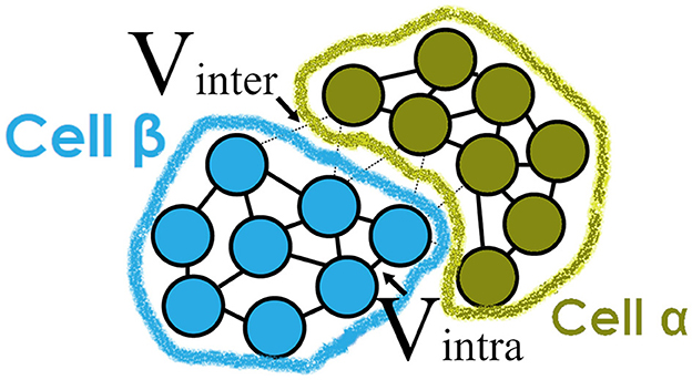
Figure 1. Representation of the physical forces defined in ScEM (Newman, 2007) between two cells α and β. Each cell is made up of sub-cellular elements whose velocity is dependent on either inter-cellular or intra-cellular forces. As the cells grow, the number of elements introduced increases until the cell is large enough to divide. The elements do not represent any of the internal signalings of the cell, but collectively they form the structure of a cell's cytoskeleton.

For each LP, elements in the border of the domain space collect information from the agents that reside in the neighboring LPs. This information is passed in the form of messages through MPI. A typical message sent between LPs would consist of information from an array of agents that are within a threshold distance from the border between these LPs. For example, if LP A is sending a message to LP B, A will first determine the direction of B with respect to A. If B is to the left of A, all elements that fall into the threshold near the left border will be identified and sent as a single message from LP A to B.

3.1.2. Signaling model

The signaling model in this simulation is driven by SBML. We use the same model as SiViT which was originally described by Goltsov et al. (2011). We deploy LibRoadRunner (Somogyi et al., 2015) to simulate the signaling model, and parameters from this model have been selected which affect the growth and division rates within the physics model, ScEM. These parameters and their links are modifiable by the user. This connection between the two models is not necessarily representative of the underlying biology but it is typical of the type of connection the domain expert might require. We provide the option to choose a combination of proteins that can affect the growth and division of a cell. The size and forces on a cell in the physics model can also in turn affect the signaling model. This is easy to modify within our framework. Domain experts can also plug in another SBML model and define how the parameters of their new model can feed into the cell physics simulation.

The tests on ARCHER did not include the signaling model. However, on ARCHER2, we have the signaling model working simultaneously with the physics model. In this complex simulation, a signaling model is instantiated for each physics cell and resides on the same LP as the physics cell. The signaling model is simulated every few timesteps, based on a simulation time threshold. The physics cell is the only external object the signaling model communicates with; for this reason, the signaling model does not need to communicate outside its own cell. Each physics cell is uniquely affected by its signaling model, and vice-versa.

3.1.3. Visualizer messages

The visualizer node (VLP) interacts with the rest of the simulation by sending an event. This event is a single message broadcast to all the affected LPs of the simulation. In this experiment, an event triggers a rollback in the simulation. The message broadcast consists of the timestamp from the visualizer to which the simulation needs to roll back. Ideally, this event could contain the type of drug and locality which will instantly affect the simulation nodes.

3.2. Initial condition setup

The simulation is made up of cells embedded within a three-dimensional Euclidean space. This space is first divided into the number of LPs available and further divided into sub-sectors to improve nearest neighbor search performance for each agent (Rapaport, 2004).

For the purposes of performance measurement, we have chosen to populate all LPs in the simulated space with densely-packed cells, replicating the conditions that would be present during the use of the system for drug discovery. This minimizes the need for dynamic load-balancing as all the LPs will roughly be hosting the same amount of agents.

Cells of uniform size are initially placed on a discrete 3D grid so that they are just touching (see Figure 2A). Each axis where the cells are aligned is displaced by the radius of a cell. One drawback to this is that partial-cell gaps are left at the edges of the simulated tissue (refer to Figure 2B), resulting in a lower load on LPs at the edge of the simulation.

FIGURE 2

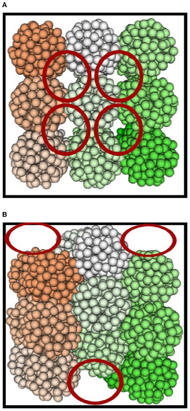
Figure 2. Initialization of 27 cells with spheroids (A) not displaced and (B) displaced over an axis. Each cell is represented by a different color and the red circles portray where the simulation load will be lesser than the rest of the densely populated space.

Once the cell's initial position has been determined, each MPI process then generates ScEM elements—presently with 128 elements in each cell. The number of elements increases as the cell grows in size, to a maximum of 256 elements. Each ScEM element interacts only with other elements within the constant interaction radius R = 10μm. Elements in an LP can be categorized as:

• Internal elements only interact with other elements within the same LP.

• Border elements interact with internal elements and also with elements in neighboring LPs.

Figure 3 demonstrates the distribution of the overall simulation space (total) into four equal LPs along with their internal and border elements based on the interaction radius $\overrightarrow{R}$. Using this approach, the new state of internal elements can be computed before any information has been received from other LPs. Only border elements must wait for information to become available. This is a latency-hiding approach: the ratio of internal to border elements can be adjusted to ensure that LPs can continue to perform computation while waiting for messages from other LPs.

FIGURE 3

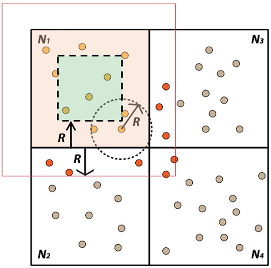
Figure 3. Representation of the simulation space in two dimensions. The complete simulation domain space is divided into 4 LPs (N_1..4). N₁ displays the internal and border elements with their interaction radius R. If an element falls within the radius R of the neighboring LPs, it will be categorized as a border element.

3.3. Simulation volume decomposition

Cells in ScEM are made up of elements that in our simulation will act as agents. We use a standard edge-exchange approach to achieve communication between neighboring LPs. Cytowski and Szymanska (2015) has divided the simulation space into a grid where each process simulates a section of the grid while keeping track of agents in its neighboring processes. Our approach is similar to this.

ScEM elements communicate with agents in a radius around it. For each element in the border of an LP, it is vital to have the agent information from other LPs. On each iteration, LPs communicate with each other and its cost largely depends on the radius of interaction R and the spatial partitioning of the Euclidean space. To statically distribute the load along the domain space, the MPI processes take control of an equal division of the simulation space. If the simulation is distributed among N processes, the total simulation space with a volume total is equally divided so that the simulated volume of one MPI process would be LP = total ÷ N.

The MPI_Dims_create function is used for dividing the space equally. Once the space has been statically allocated, the MPI processes will decide the agents simulated within it. This method maps well with the topology of how the LPs will be physically positioned close to each other.

When the simulation is running there are two types of communication between LPs. The first type is the selective data required by bordering processes. Here, minimal data is collected from each agent in the bordering regions and sent to the MPI processes that require it. The second type of communication—migration—is triggered when an agent's position moves from the authoritative region of one LP to another. Here, the agent's state and all its histories are transferred from one process to another. This will ensure that each agent is in the right LP to receive the information it needs to compute the next time step. Rousset et al. (2015) have identified the need for agent migration to ensure smooth proceedings of an ABM while using HPC clusters and MPI.

The frequency of migration needs to be minimal because this transfer may stall the simulation. Stalling is essential as migrating agents could fall into the interaction radius of an internal agent. Without having the migrated state of an incoming agent, the internal agents would not have all the information they need at the beginning of the time step which in turn would affect the determinism of the simulation. If the maximum allowed displacement of an agent per time step is known, it will be possible to predict which agents will not be affected by any incoming migrating agents. Latency-hiding methods can then be used to improve the performance of this simulation.

A part of the communication overhead depends on the number of nodes with which an MPI Process needs to communicate. This is decided by the neighboring processes that surround an individual simulation space LP. In ScEM, on each iteration, the processes require two phases of communication. This is simply because a timestep in ScEM consists of two integration steps, each step termed as a half-step. To compute the integration state, each element as designed in ScEM requires the state of all the elements around it (within the R = 10μm threshold). This requires the communication of the minimal border data twice and migrating agents twice across the LPs for each timestep.

3.3.1. Size of messages

Spatial decomposition subdivides the simulation space into smaller sections which are simulated on separate MPI ranks (termed as LPs). An element in ScEM can only interact with other elements around it that lie within the 10μm range, thus the threshold for bordering agents can also be safely presumed to be a distance of 10μm away from the border of the enveloping LP border. As ScEM is a physics model of a cell, each element takes up a certain amount of space within the simulation. This can be calculated as follows: the radius of a cell is R = 10μm and the number of elements in a cell is N_cells = 128, roughly every element takes up the volume of 32.72μm³.

Each LP on MPI takes up ~384, 500μm³ simulation space (LP). This volume was determined by running preliminary tests to find an ideal size of the simulation (refer to Section 4.2 for more information). Estimating the shape of the LP as a cube, we get a single side of 72.416μm. As we have one side, the number of elements that can reside on the bordering elements can also be calculated as we know the dimensions of the bordering threshold cuboid. The volume of a bordering cuboid can be calculated using 72.416 × 72.416 × 10 = 52, 874μm³. If we divide this by the volume a single element takes up, we get the number of cells that reside in the bordering elements: ~1, 652 elements.

First, all the elements to be sent are identified and their data is collated in an array-like structure. The information sent to capture the state of each element consists of 112 bytes of data. Each message sent to a neighbor could range from (0 → 1652) elements based on the density of the simulation. Worst case scenario, the size of a single message would be 185,024 bytes or 185 KB. Messages are sent from an LP to all its neighboring LPs. The number of Neighboring LPs can range from (8 → 27) in a large-scale 3D simulation. With 27 neighbors, an LP will send and receive ~5 megabytes on each time step. These parameters can be modified without compensating for the correctness of the models. Newman (2007) explains the set of parameters in ScEM and their effect on the accuracy of the cell-physics model.

3.4. Communication within the LPs

With a simulation scaling well by limiting the interaction of the LPs to its immediate neighbors, focus needs to be brought to the visualizer and collection of selective data. The Visualizer LP (VLP) may be further away from the frustum of the simulation which increases the time variability for receiving these messages. As the messages are being sent in a non-blocking method, the latency will not affect the speed of the running simulation, but the latency may be visible to the visualization user.

To establish a real-time interaction with the distributed simulation in spite of being on an older time-step, this project uses the following synchronization strategy.

3.4.1. Communication between simulation nodes

The simulation is now divided into two types of LPs, Simulation LPs (SLPs) and Visualizer LP (VLP). The simulation LPs will continue to operate synchronously while communicating with other SLPs surrounding it. SLPs store a history of the states of each agent and communicate with the VLPs at regular intervals. SLPs communicate with VLPs in a non-blocking approach which makes the simulation independent of the visualizer's speed. The flow of the simulation on a single Simulation LP for the ARCHER (simple) simulation is explained in Figure 4 where the initialization step has been explained in Section 3.2. The system then checks which integration step has been reached by ScEM followed by sending and receiving of the border and migrating elements. There are 2 synchronous steps W1 and W2 where the simulation may stall until all the required information has been received by the SLP. Additionally, Figure 5 explains the communication patterns between multiple SLPs where W1 and W2 are reiterated. On ARCHER2, the same simulation is compounded with cell growth, division, and signaling.

FIGURE 4

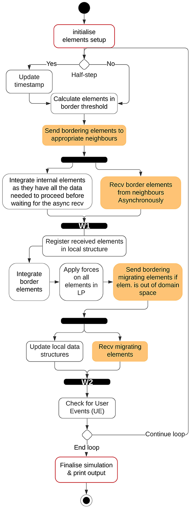
Figure 4. Flow of the simulation time-step within an SLP on ARCHER. In ScEM, there are two integration steps for each timestep, within the simulation space, each integration step will be termed as one half-step. W1, W2, and UE are points where the simulation might need to wait until all data from neighboring LPs has been received. This is better explained in Section 3.6.2.

FIGURE 5

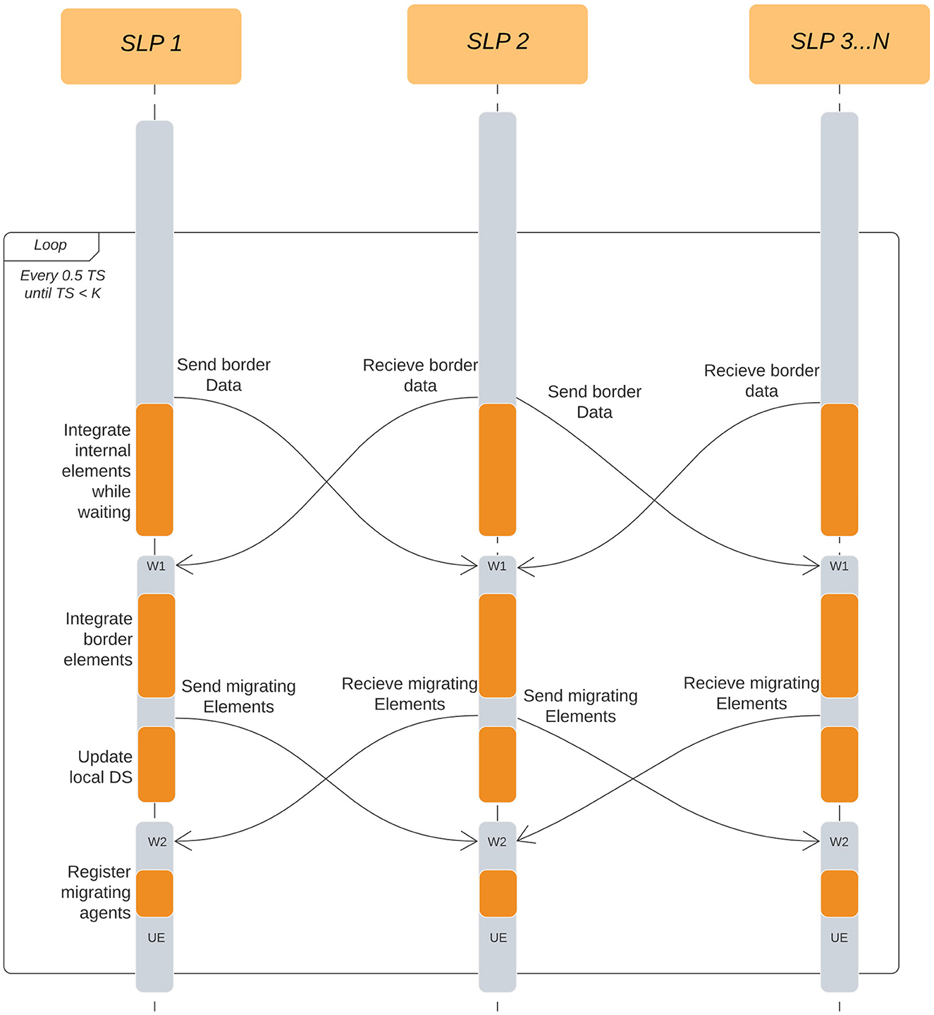
Figure 5. Interactions between SLPs on each half-time-step. K is the total number of time steps we run the simulation for. W1 and W2 are two independent wait points in the simulation where LPs are waiting for information to be received from other LPs. W1 is waiting for the state of bordering elements, while W2 is waiting for Migration elements. In both cases, the simulation cannot proceed until all information has been received from the neighboring LPs. UE is a point in the simulation which checks for incoming User Events.

3.4.2. Communication between visualizer and all SLPs

SLPs send data to the VLP at a set interval of time steps. The interval can be dynamic to accommodate for variance in the simulation speed, but for the scope of this paper, we will keep the visualizer update interval a constant (ΔT_i = 100). The VLP maintains a list of SLPs to communicate with. If the SLP is within the frustum of the visualizer, the SLP will send the state of the agents within the viewport to the VLP. This list is updated as the visualizer moves from one part of the dense simulation to another.

On every visualizer interval timestep, the SLPs in the update list only send the current state of their agents, no histories are sent. The visualizer receives this data every ΔT_i and visualizes this to the user in the received order. Figure 6 explains the communication between a VLP and multiple SLPs.

FIGURE 6

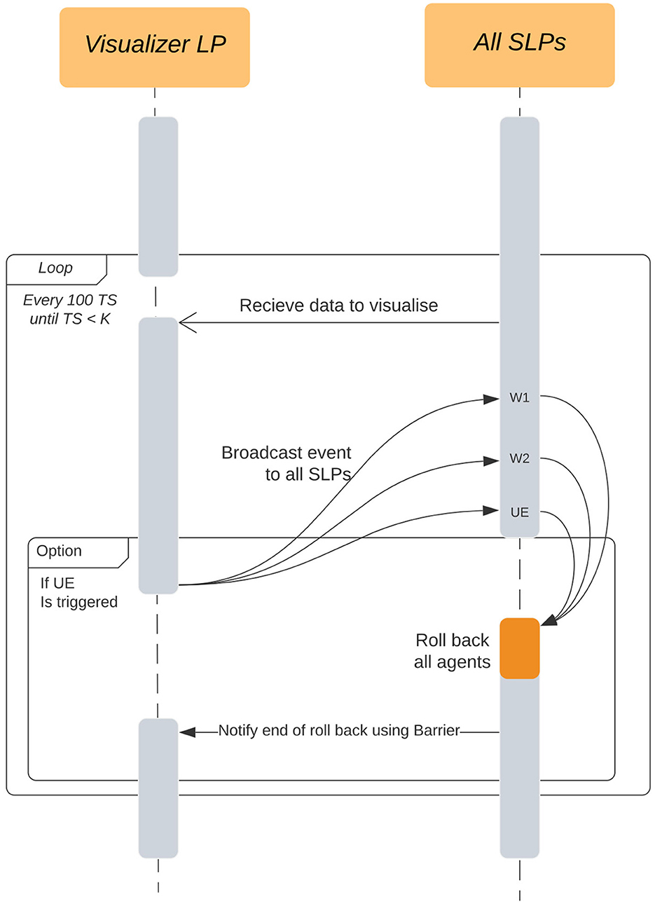
Figure 6. Interactions between the Visualizer LP (VLP) and all the Simulation LPs in the simulation. The event is broadcast from the visualizer but can be intercepted at any of the simulation wait points (W₁, W₂, UE) and immediately rolled-back to avoid deadlock. These wait points are the same as the ones found in Figure 5.

In our implementation, we use a fixed frustum to conduct our experiments.

3.5. Roll-backs for real-time interaction with the 4D tumor

The VLP is responsible for sending user-defined interactions to the simulation. This method achieves real-time simulation interactions using an optimistic IO approach (Jefferson, 1985; Hybinette and Fujimoto, 2002) where the state of each agent in the SLPs is saved for every time-step that has not yet been received by the VLP. When the VLP broadcasts an event (E_t) to the SLPs, they roll back every agent to the notified time-step (t) and then progress with the simulation.

With this method, a majority of the simulation takes place using a conservative method, whereas only the user interactions will be handled using an optimistic approach. The number of states stored for each LP will be limited to the distance between the current SLP timestamp and the time-stamp of the VLP (T_vlp). To limit the memory overhead caused by the histories stored, we can further limit the simulation in a conservative approach if the SLPs' time-stamp exceeds the VLP time-stamp by a high threshold. When this condition is triggered, the SLPs will wait for the VLP to progress—effectively combining the conservative and optimistic approaches.

The depth of history saved for each agent would add an overhead to the memory required by an LP. In ScEM, the elements store position data, velocities, cell-type descriptors, strength, and indexes for their parent cell. A history state is stored at each visualizer update interval. The number of history states required can be reduced if the update interval is increased. Each agent has a Maximum History allowance, after which the SLP will wait until it is safe to save another state.

The histories of an agent will be migrated when the agent crosses the border between two SLPs. This can affect the amount of data transferred over the network while migrating agents. However, based on our observation, this condition is triggered less frequently in our implementation of the simple and complex cell simulation.

For the case of drug discovery, end users will be able to pause the visualization, analyze the changes and events that need to be administered and resume the simulation, getting results back within a reasonable time frame after dispatching the event. From our observation in SiViT (Bown et al., 2017), a reasonable round-trip time frame for domain experts while interacting with a single cell was ~1409ms.

3.6. Communication and overhead optimizations

Agent-based parallel simulations face some common bottlenecks because of the distributed memory hardware architecture. In this section, we describe how we alleviate these issues.

3.6.1. Nearest neighbor search

To optimize the performance of the simulation, the neighbors are subdivided into grids using the particle-in-cell method (Rapaport, 2004). This method is known to have the computational complexity of O(N²) where N indicates the number of agents in the data structure. We limit the number of elements N in a data structure by subdividing the space into smaller particle-in-cells. Tree-based algorithms can add a benefit to neighbor searches. Cytowski and Szymanska (2014) uses such an algorithm for finding neighbors in a large-scale agent-based cell model not very different from ours. However, in a tree, at each step, there is an added cost of maintaining and potentially rebuilding the structure.

3.6.1.1. Neighbors and communication bottlenecks

Even though a cell in ScEM forms the shape of a sphere, in this simulation the total domain shape (total) is a cube. Using a cube, the volume of an individual LP (LP) and the MPI_Rank of its immediate neighbors can easily be determined from their position in the grid.

The shape of the LP affects the neighbor searches for that LP. The interaction radius $\overrightarrow{R}$ of an element in ScEM is always constant. When dividing the total equally among LP processes, the shape of the divided volume (LP) is set as a cuboid of unequal bounds. This affects the number of neighbors an LP would communicate with and the latency hiding technique within each LP, i.e., internal and border elements. An LP can only communicate with neighboring LPs that share a border with it. Based on how total is divided, an LP can have a variable number of bordering neighbors. We use the MPI_Cart_create function to equally divide total into . The ideal shape of LP would be a cube but that will only be possible when the total number of LPs is a perfect cube. The greatest bottleneck would be when LP is a prime number. In this case, by using the MPI_Cart_create function, the overall space will be divided into (LP,1,1) across the dimensions. Figure 7 portrays this in two dimensions. When the dimension of LP is smaller than the radius of interaction, it would not have enough volume to host internal elements. This would invalidate the latency hiding technique in an LP.

FIGURE 7

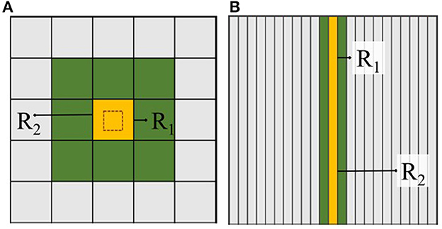
Figure 7. 2D total of square dimensions is divided equally where (A) is 5² and (B) is a prime number. R₁ and R₂ represent two radii of different lengths which affect the number of neighbors an LP communicates with. This number increases with the order of the specified dimension.

3.6.2. Deadlock avoidance

Simulation LPs send data between them to ensure that agents at the start of a timestep have the information they need in the Euclidian space around them to continue the simulation. In MPI this is done by sending messages using a non-blocking approach. In the unlikely event that no information is required to be sent, we use a null message to allow the simulation to proceed.

Figure 5 shows how a simulation node will communicate with surrounding simulation nodes. Here W1 is a wait point where the simulation might be stalled for information from neighboring LPs. While the simulation proceeds in a non-blocking approach, an MPI rank posts an IRecv and then continues to process internal elements. After processing the internal elements, we test if the messages from all neighboring LPs have been received. If not, the simulation will wait at W1.

Similarly, for migrating elements, the simulation will wait for all the messages from the neighbors to be received at wait point W2. See Figure 4 to better understand the flow of the simulation.

This non-blocking communication is generally easily achieved by using a combination of MPI_Probe and MPI_IRecv for messages which can be anticipated. However, non-blocking protocols can take control away from the program. We are also working with messages that are not anticipated—real-time user events. These are also sent in the form of a message from the visualizer to the rest of the simulation.

If a user event is dispatched from the visualizer to the rest of the SLPs, each SLP might intercept this message at different points in the simulation. This means that SLP_A could be stuck in wait point W1, while the message it is waiting for will not be received as the neighbor has already intercepted the user event and has rolled back, thus SLP_A would be in a state of endless wait for a message that will not be delivered.

We resolve this by testing for the user event every time there could be a potential wait point between SLPs. We do this by looping through all the neighbors and testing if a message has been received using MPI_IProbe and MPI_Test. This gives us the flexibility of having a variable message size by using IProbe (thus, a null message which is faster to deliver), and MPI Test instead of MPI Wait would be done intermittently while waiting and receiving data from neighbors. This can also be done using MPI_Waitany; however, that would take away the possibility of sending a null message as the use of MPI_Probe would take control away from the program and newer MPI_Waitany calls will not be invoked.

Looking at Figure 6, we intercept the User Events (UE) at three points in the SLPs, W1, W2, and UE.

3.6.3. Message cancellations

Our implementation of this simulation warrants the rare use of MPI_Cancel. When an SLP successfully intercepts a message from the visualizer, before rolling back its current state, the simulation would have to cancel any messages sent out or incoming messages that would have been sent out prior to rolling back. This ensures that any message residues do not affect the state of the simulation after rolling back and all message queues are flushed for a fresh start after the rollback.

Generally, messages sent just before rolling back can be discarded. However, elements that migrate from one LP to another are transferred in the form of a message too. If this message is discarded, it is possible that an element with its history is lost and hence, cannot roll back that particular agent.

We tackle this by recovering this message on the sender or receiver end. On the sender end, we cancel the sent message using MPI_Cancel and then if the cancel succeeds (the message has not been sent yet), we recover the element details from the send buffer before clearing it. Similarly, on the receiving end, if the message has already been received in the Recv buffer, but not yet copied into the list of elements, we recover the message on the receiving end and add it to the list of elements at the receiving LP.

At the point of rolling back, each element's state is rolled back and its position is altered. Immediately after rolling back, all the elements in the wrong LPs will be migrated back to their authoritative LPs.

Cray MPI on ARCHER and ARCHER2 use the eager protocol to transfer messages between nodes. In the eager protocol, messages are sent to the MPI rank even though a matching Recv has not been posted. These messages are stored in the receive buffer until a matching Recv is posted. This means that even though a message is canceled on the sender's end, there can be residues on the receiving end. For our simulation, this led to problems as messages that had been canceled were still being received out of order after rolling back the simulation. We post a probe and a blocking MPI_recv for ANY_RANK and ANY_TAG to flush these messages. This ensures that the Recv buffer has been completely cleared out before rolling back the simulation. This can also be solved using a buffered send/recv.

3.7. Verification

Maintaining the deterministic nature of the scientific simulation is essential. In spite of distributing the simulation over N processes, the accuracy of the simulation output needs to remain intact. We must ensure that the simulation is initialized consistently and that its results are the same regardless of the distribution structure.

To initialize the cells in a reproducible way, the ScEM elements are initialized using a random seed which is derived from the parent cell's index. With the help of this, the cells can be initialized in any node while having the same initial state for each of its elements. As an alternative, we could read the initial states from a file. To ensure that the consistency of the simulation has not been compromised, the simulation was run with a range of different sizes and numbers of LPs. The most sensitive output from ScEM's calculations (because it depends numerically on all the other parameters) is the positions of the elements. After running the simulation for T time steps, the absolute positions of all cell elements are collected on a single node and written to a text file. The relative error between the expected and acquired results are calculated. With our final testing, we have observed that the relative error on every test case scenario is an absolute zero. The benchmark for expected results is obtained by recording the positions of the cell elements after running the simulation for T time steps on a single LP without any distribution. This benchmark is compared using a diff tool to the output of the different test case scenarios. With an increasing number of MPI Processes (N = 1, 8, 16...256), the simulation was executed for (T = 5000) iterations. Tests were also conducted to ensure that the results of the simulation remain deterministic after an event has been communicated during user interaction. To test this, an empty event is dispatched which does not make any alterations to the simulation but triggers a roll-back in all the SLPs. The same range of simulation sizes was tested both with and without synthetic events.

As the signaling and cell physics simulations use floating-point computations, there is potential for numerical error (Cassandras, 2008) based on the ordering of floating-point computations. This error was not observed in the test cases that we ran as the elements are sorted in each LP using their unique identification number. This form of sorting ensures that in spite of spatially distributing the simulation, the order of floating point calculations will remain the same, thereby giving the same deterministic results on each run.

4. Results

The features of the HPC simulation framework to be evaluated are scalability, deterministic verification, real-time user interactions, and deadlock avoidance.

This section explains the four tests that were conducted first on an existing HPC unit—ARCHER in Edinburgh (EPCC, 2014) which has 118,080 CPU cores available to deploy the simulation on. After the decommissioning of ARCHER in 2021, we updated our simulation and ran the tests on its successor, ARCHER2 (EPCC, 2014) which has 750,080 CPU cores. Each test summarizes the scalability of a different aspect of the simulation to answer the questions posed in Section 1.2 which leads up to how the user interaction would scale with a higher number of nodes.

4.1. Hardware of the HPC systems used

ARCHER was commissioned in 2014 and uses the Cray XC30 system. ARCHER consists of 4,920 nodes and each node has 24 CPU cores of 2.7 GHz (2 NUMA regions with 12 cores each, 2 × Intel E5-2697 v2). Each node of ARCHER has 64 GB of memory and employs the Aries interconnect with a bi-directional bandwidth of 15 GB/s per node.

ARCHER2 was commissioned in 2021 and uses the HPE Cray EX system. ARCHER2 consists of 5,860 nodes and each node has 128 64-bit processors of 2.25 GHz (8 NUMA regions with 16 cores each, 2 × AMD EPYC Zen2-Rome 7742). Each node of ARCHER2 has 256 GB of memory and employs the HPE Cray Slingshot interconnect with a bandwidth of 100 GB/s per node bi-directional. Even though ARCHER2 supports hyperthreading, we do not use it for our simulations as we observed an improved speedup in performance by using the individual physical cores.

4.2. TEST I: speed-ups and verification

The results from this test answer questions one and two earlier posed in the objectives (Section 1.2).

(Q1) Is the simulation deterministic, and does it produce the expected results irrespective of domain decomposition?

(Q2) Does the simulation scale strongly while keeping the problem-space constant and increasing the computational resources?

While simulating the same number of cells in constant total, we increased the number of MPI nodes LP = {1, 8, 16..256} to divide the workload of the simulation. The time taken for a single time step T_LP is recorded after simulating T = 5, 000 steps. total does not change, but when distributing the work, the volume of a single LP (LP) will decrease when LP increases. After a certain point, the interaction radius of an agent will be large enough to require information from the second-degree neighbors in the grid. This causes a major overhead in the simulation as there will be no internal elements to hide the latency of incoming messages. From the results in Figure 8 we can see at LP = 8192 the simulation slows down as there are very few elements that reside within an LP, only ~¹/₅^th of a cell is being processed on each LP.

FIGURE 8

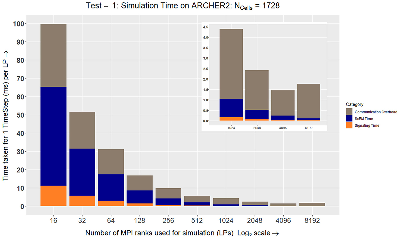
Figure 8. On ARCHER2, we see how the simulation speeds up while measuring the three major aspects of our complex system: ScEM, Signaling, and Communication Overheads. At LP = 8192, the communication overheads outweigh the amount of time required to simulate ScEM as only ~¹/₅^th of a cell is being processed on each LP. For Tests 2, 3, 4, and 5, we used the size of the simulation volume LP = 72³μm³. This value was obtained from LP = 48 from the graph above. This is because the amount of time taken to simulate the cells is ≃ the communication overheads. Approximately 40 cells were simulated in this volume (). The inset figure here is a zoom-in on the last four data points.

This test helps determine the optimal balance between internal and border elements in an LP. We found that for hiding the local latency, after a point, reducing LP will have a negative impact on the performance. From the results of this test, we determined a constant volume LP which held enough agents internally for efficient latency hiding in our local setup. This value will be used in the tests below to see how our simulation scales. Essentially, in this experiment, we are keeping the problem size constant while increasing the number of processors.

4.2.1. Test I—ARCHER

The simulation of 10³ cells shows strong scaling results (Figure 9A). The simulation gets faster with an increasing number of LPs. ARCHER uses a network called the Cray Aries Interconnect where the latency between MPI nodes is ~1.3μs which is much faster than an Ethernet connection (EPCC, 2014).

FIGURE 9

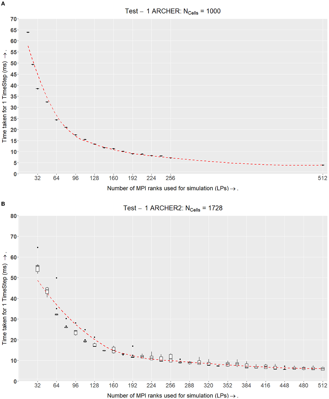
Figure 9. Test I. This experiment tests for an ideal size in the simulation volume LP where the ratio of inner-elements:border-elements would be balanced. This volume for LP is used in the following experiments. (A) Benchmark results from the ARCHER setup. The x-axis shows the number of MPI processes used and the y-axis shows the total amount of time in milliseconds to compute one timestep of the simulation. For this setup, each simulation band is run 4 times for 5,000 timesteps. The number of cells N_cells remains constant at 1,000. This simulation shows strong scalability results. The dotted line in all the figures is the line of best fit calculated using the Loess method for all the points plotted in a graph. (B) ARCHER2 results which demonstrate that in spite of the inclusion of growth, division, and the signaling model, the simulation scales well and maintains a similar computation speed as ARCHER in (A). Note that the number of cells being simulated here is higher than ARCHER. Here 12³ cells are being simulated; however, the main goal of finding an ideal size LP remains the same.

From these results in Figure 9A, there appears to be an advantage in speedup after further subdividing the simulation's domain space. In spite of reaching a second-degree neighbor threshold, the communication latency is very small because of which a speedup in overall performance is prominent. This test verifies that supercomputers that have a fast interconnect such as ARCHER can lead to computational speedups as long as the communicating MPI nodes are physically close to each other.

When plotting a speedup graph for this test (Figure 10A), we notice that the speedup value increases linearly with up to 512 LPs.

FIGURE 10

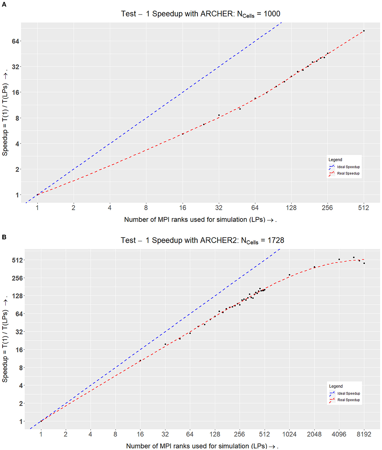
Figure 10. Speedups within Test I on ARCHER and ARCHER2. (A) Speedup of the simulation on ARCHER where Speedup = T₁÷T_LP. Here the ideal speedup indicates that doubling the number of processors would double the speedup of the simulation. This is in an ideal world where there would be no communication overheads. (B) Speedup of the simulation on ARCHER2 where Speedup = T₁÷T_LP. Here we stress-tested the simulation at a higher number of LPs to see where the scalability curve starts to drop. At LPs = 6,144 (each LP here would simulate ~¹/₃^rd of a cell), we achieved optimal performance, after which the speedup values started to drop as the number of elements simulated per LP are very low at LPs = 8,192 (each LP here would simulate ~¹/₅^th of a cell).

4.2.2. Test I—ARCHER2

The experiments conducted on ARCHER2 were held approximately a year after the ARCHER experiments. ARCHER was decommissioned in January 2021, and ARCHER2 was installed soon after. After obtaining the results from ARCHER, we made a few additions to our simulation. Originally, the ARCHER simulation did not accommodate growth and division within the physics model. The tests on ARCHER2 on the other hand, implement growth, division, and the signaling model. The results that we obtained on ARCHER2 can be found in Figure 9A where we simulated 12³ cells.

We plotted the speedup values for the two simulations which can be seen in Figure 9. The simulation on ARCHER2 in Figure 10A shows that the simulation stops speeding up after LPs = 6144. We broke the simulation down even further and recorded the amount of time it took for each segment of the simulation (ScEM, SiViT, and Communication Overheads). The results for this can be seen in Figure 8. Here, at LPs = 8, 196, each LP hosts only ¹/₅^th of a cell, and the communication overheads no longer help speed up the simulation.

The first experiment demonstrated that the number of cells per process could be adjusted to hide the communications latency in a cluster while using non-blocking communications.

4.3. TEST II: scaling up the 4D tumor simulation

The results from Test II answer the third question posed in the objectives (Section 1.2).

(Q3) Does the simulation scale strongly as we increase the number of cells in a simulation while increasing the computational resources?

Having found a constant volume that balances inner and border elements efficiently, this test checks whether this algorithm scales well with a larger number of cells. In this test, we keep the agent density and volume LP of an LP constant while increasing the number of cells and overall simulation space. This ensures that the total number of cells simulated per LP remains approximately the same in spite of increasing the number of LPs at scale. To keep the agent density constant, the side of a total simulation volume (a cube) S_total is calculated using Equation (1) where LP has been determined in the previous test. Here, N is the number of LPs being used for the simulation.

The number of cells N_C populated for each test case is given by Equation (2) where R_C is the radius of a cell defined by ScEM. This will lead to residual gaps on the border of the simulation as explained in the initial condition setup section.

$\begin{array}{ll}{N}_C={\lfloor \frac{S_{total}}{2R_c}\rfloor }^3& (2)\end{array}$

The time taken for each time step T_LP is recorded while changing the N_C(Range: 2³...13³), S_total and increasing the LPs (where N = 1, 16...272). Keeping LP constant, we are ensuring that each LP has an efficient balance of internal and border elements. To understand whether the results are scaling well, in Figure 11A, we normalize T_LP by N_C for each test case. This gives us the time taken at each time step by a single cell in the simulation.

FIGURE 11

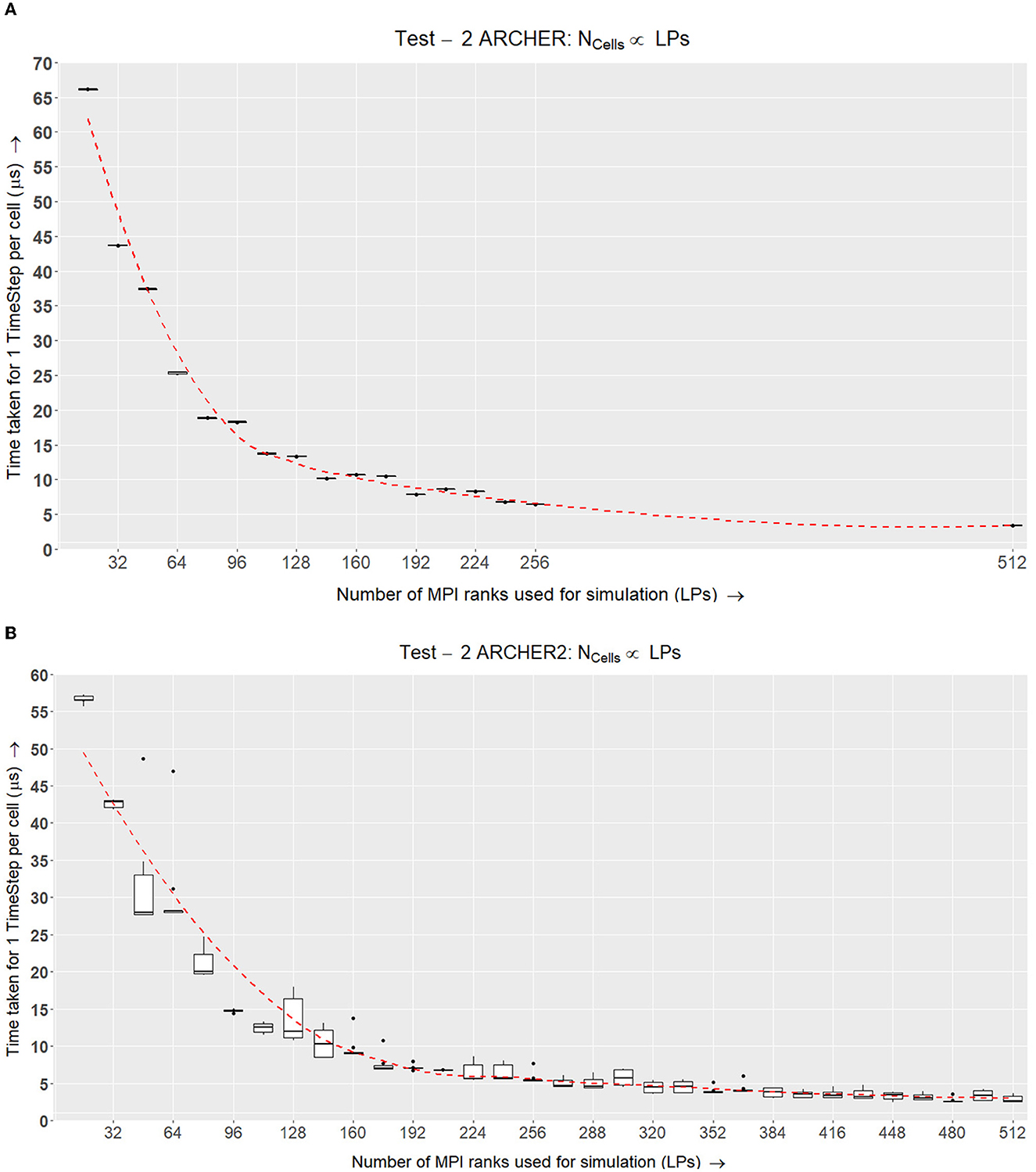
Figure 11. Test II. This experiment increases the number of cells and LPs linearly using Equations (2) and (1) to populate the simulation space. This is tested over a selected number of LPs and the normalized time taken to simulate a single cell for one timestep is recorded. (A) Box plots representing the benchmark results for Test II on ARCHER where the number of cells increases with the number of LPs. Each simulation was run 6 times for 1,000 time-steps and the time taken for each time-step was recorded and normalized against the number of cells simulated. (B) ARCHER2 results for Test II demonstrate the scalability curve for the simulation over up to 512 nodes.

4.3.1. Test II—ARCHER

In Figure 11A, the results from running this test on ARCHER show that the scalability curve is improving over the number of LPs because of the faster Interconnect between MPI Nodes. The additional experiment carried out for 512 nodes further emphasizes that the simulation scales well when simulating a larger number of agents with equivalent additional resources.

4.3.2. Test II—ARCHER2

The tests conducted on ARCHER2 (Figure 11B) were of a similar setup as ARCHER, except that the number of cells simulated per LP was higher in ARCHER2. The number of cells is scaled up linearly with an increasing number of LPs. As this test was conducted after the ARCHER experiments, we were able to add more data points to show the scalability curve across 512 LPs. The amount of time taken to simulate an LP per timestep is decreasing over time which shows strong scaling results over 512 LPs.

The second experiment showed that the simulation scales with an increase in the number of processes while linearly increasing the number of cells.

4.4. TEST III: scaling up when a VLP is connected

The results from this test answer the fourth question earlier posed in the objectives (Section 1.2).

(Q4) What overhead is introduced by the visualization LP?

To determine whether communication with the visualizer has any effects on the scalability of the simulation, the previous test setup (Section 4.3) is repeated with a visualizer plugged in. Here the visualizer is an additional LP that receives data periodically from selected simulation nodes. The VLP is viewing a part of the running simulation where it receives data at a constant time-step interval.

4.4.1. Test III—ARCHER

On ARCHER and ARCHER2, this test requires some alterations. Since both supercomputer systems use batch scheduling and have limited connectivity to machines elsewhere on the Internet, it was not practical for us to evaluate an interactive graphic visualizer in these experiments. Instead, the functionality and performance characteristics of a visualizer were emulated on a CPU MPI node. The data from the required nodes are sent to this emulated VLP and after a constant wait time, this VLP will send out more MPI_Recv requests for the next set of data to be obtained for visualization.

Figure 12A displays similar results to Test II in Figure 11A where the time taken scales well with the simulation while an additional constant time is added for each configuration.

FIGURE 12

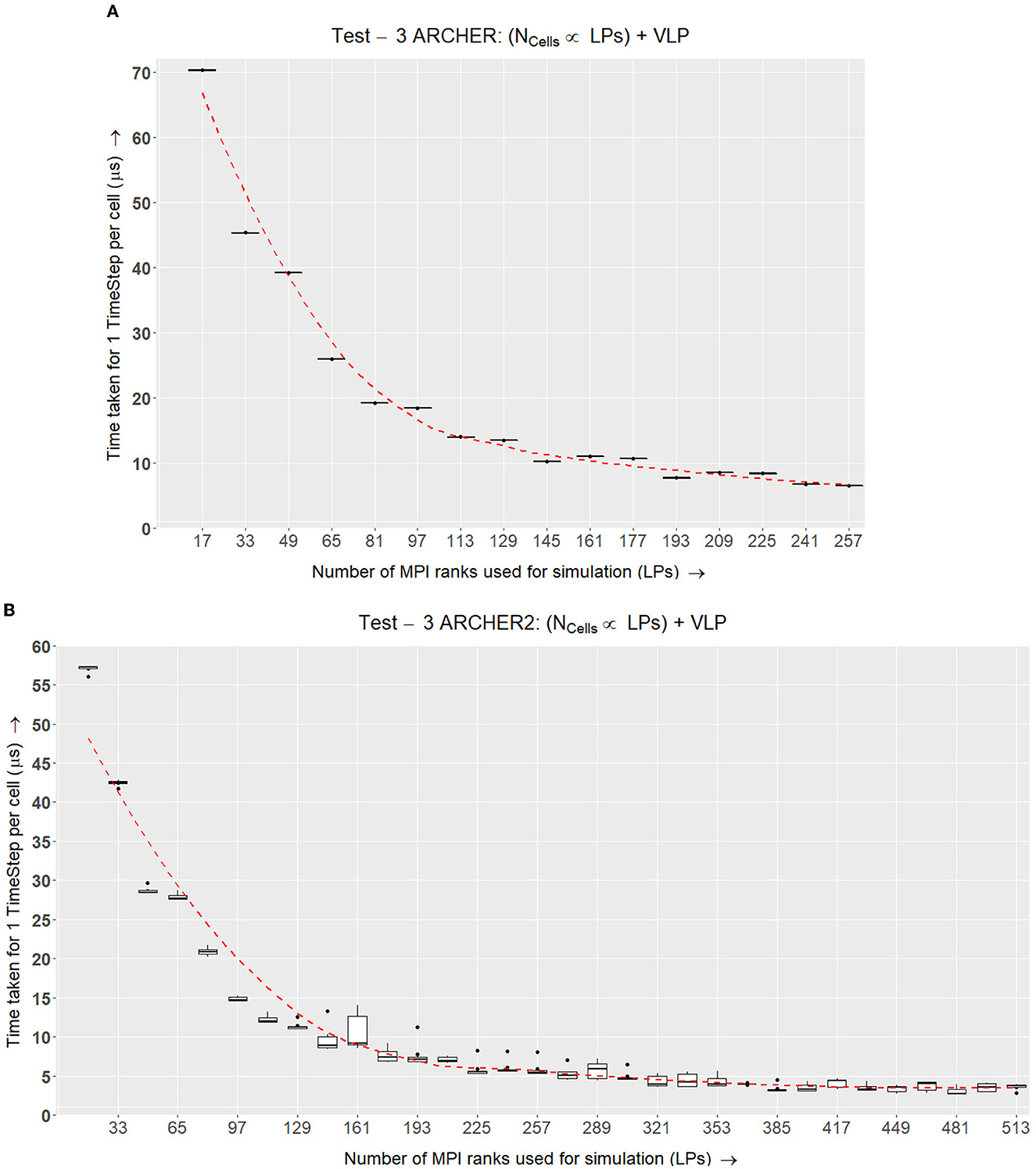
Figure 12. Test III. This experiment is similar to Test II (Figure 11) with an addition of a visualizer to the simulation. Selected simulation nodes send information to the visualizer every few timesteps. (A) Box plots representing the time taken for one cell per time step on ARCHER while increasing the number of LPs and cells in the simulation and also adding a visualizer that selected simulation nodes regularly send data to. Here the last node is the visualizer node which is why the data points are denominations of (16 × N)+1. (B) ARCHER2 results for Test III, which is a similar setup as (A) however, this simulation accommodates growth, division and the signaling model on ARCHER2.

4.4.2. Test III—ARCHER2

The results for this test on ARCHER2 in Figure 12B show that incorporating a visualizer does not adversely affect the scalability of the simulation.

The third experiment showed that the simulation scales reasonably to the bounds of our cluster size when a visualizer is plugged in without dispatching any user-defined interactions.

4.5. TEST IV: scalability of the 4D tumor simulation for real-time user interactions

The fourth set of our results measures the round trip time of a dispatched user event from the visualizer node. This answers the fifth question earlier posed in the objectives (Section 1.2).

(Q5) How long is the round-trip of a real-time user event from the visualizer node?

The same setup from the previous tests (scalability of SLPs when a VLP is connected, Section 4.4) is used for this test with an addition of user events being dispatched.

When an event is dispatched by the visualizer, a global communication is triggered which broadcasts a message to all the SLPs. Once this message is received by each SLP, a roll-back is triggered which changes the state of each agent to match the required timestamp. Once an SLP rolls back and completes a cycle of simulation, it sends the new set of simulated data to the VLP. We measure input-feedback latency by recording the amount of time taken from the initial broadcast until the receipt of the next visualization data.

For every test case, 25 synthetic events are sent and the response time of the new visualization data is measured.

In our MPI-based implementation, an SLP might catch a user event successfully while its neighboring SLP could be waiting for data from its neighbors (i.e., a neighbor that has already rolled back). This could lead to deadlock. Our way around this problem is by testing for a user event message while waiting for any incoming message. This can be implemented using the MPI_Waitany function and user events can be caught and handled without the prospect of deadlock.

In our current implementation, we are using a global synchronization (MPI_Barrier) to ensure that all the messages are received and rolled back without facing deadlock.

4.5.1. Test IV—ARCHER

When deploying this experiment on ARCHER, the same changes to the VLP are made as explained with Test III.

The results in Figure 13A show that the response time for a user event can vary based on the number of LPs and the type of network the simulation is running on. ARCHER and ARCHER2 make use of Cray Aries Slingshot networks which are optimized for collective communications. EPCC has evaluated the communications with MPI_Barriers on ARCHER at scale (Quan, 2014) and recorded that the latency between nodes varies if the nodes are in different cabinets or groups. Our results from Figure 13A show that the simulation scales as well as the underlying network hardware, where if the simulation is scheduled within the same cabinets of the HPC unit, the response time is similar.

FIGURE 13

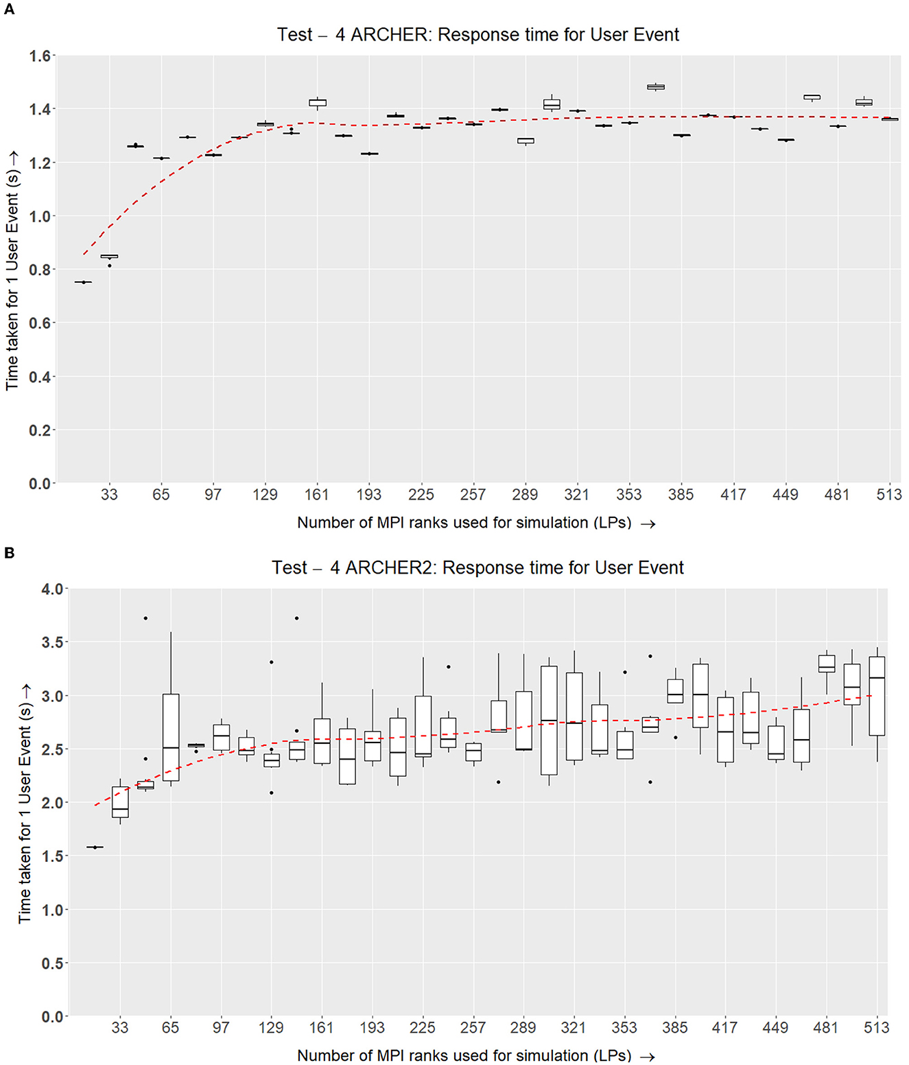
Figure 13. Test IV. This test shows the roundabout time from the point of dispatching a visualizer user event to the point of response from the simulation nodes with new data after rolling back the simulation and applying the requested changes. (A) Each simulation band is run 6 times with 5,000 time-steps. At regular intervals, 25 user events have been sent and their average response time at the next visualizer update, after successfully rolling the simulation back is recorded. The number of cells simulated is linearly scaled up with the number of nodes (Similar to tests 2 and 3 in Figures 11, 12, respectively). (B) ARCHER2 results for Test IV, which is a similar setup as (A) however, this simulation accommodates growth, division, and the signaling model on ARCHER2.

4.5.2. Test IV—ARCHER2

The results from Figure 13B show that the user event response is consistent across the number of nodes, and the simulation scales according to how it is scheduled on the compute nodes. The overall rendezvous time for a user event is roughly between 2 and 3.5 s which remains consistent across 513 LPs.

The number of cells simulated per LP on ARCHER2 is higher than the ones in ARCHER. This is because the ideal LP is different in both simulations. Because of this, the overall response time and data sent between the visualizer and simulation nodes are uniformly higher in ARCHER2.

The fourth experiment demonstrated that the response time for user interaction scales well with the network latency and underlying hardware, giving us a reasonable response time for a user event.

4.6. TEST V: ARCHER—Simulating up to one million cells

With the four tests conducted above, we get a good idea of how the simulation would scale on a smaller level with which we can predict an estimate of how the simulation will scale on the targeted hardware. However, this does not answer the original question.

(Q6) Can the system simulate a typical cancer spheroid (1 million cells) via interactive simulation?

To answer this question, a final simulation was conducted which is similar to Test IV.

4.6.1. Test V—ARCHER

In Figure 14A, we are testing the amount of time taken to simulate ScEM Physics elements when we scale up the simulation from N_c ranging between N_c = {1, 331...1, 000, 000}. The number of CPU cores used to simulate one million cells is 21,953. Here, the Domain size of the base node was increased to accommodate more agents in a single MPI rank. Here, the size for one LP (LP)is now exactly the same as what has been used for ARCHER2. As one cell consists of 128 → 256 elements, we are simulating over 128 million elements.

FIGURE 14

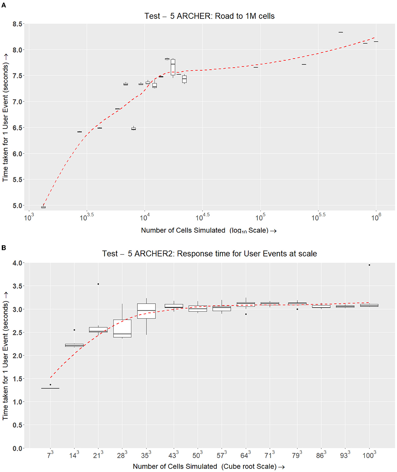
Figure 14. Test V. This experiment is similar to Test IV (Figure 13) but at a larger scale. Here, we compare the time taken for the response of a user event depending on the number of cells being simulated. This requires LPs ranging from [33 → 21, 953]. (A) After obtaining preliminary results for the final tests in Test IV, we have scaled up the simulation to fit within the limits of ARCHER. Here, we are simulating up to one million cells over 28³ CPU cores (~22, 000). (B) The same setup that was used for ARCHER in (A) is being simulated on ARCHER2 with the inclusion of growth and division and the signaling model. ARCHER2 tests were conducted a year after ARCHER tests. The data points selected in ARCHER2 were better planned to fit the log scale well and give a more insightful picture of how the simulation scales.

The results in Figure 14A show an upwards trend in response time when more agents are simulated over a large number of LPs.

4.6.2. Test V—ARCHER2

The final test on ARCHER2 incorporates cell physics (ScEM) and cell signaling (SBML Model). ScEM in this implementation is fully featured with growth and division also implemented. We simulate this complex system on a range of LPs while increasing the number of cells simulated. In Figure 14B, we can see a slightly better scaling ratio compared to ARCHER. where even at a larger number of nodes and cells, the user event response is consistent at approximately 3 s.

Additionally, we measured the communication overheads for this simulation to see how the simulation scales while sending user events. These results in Figure 15A demonstrate that the input-feedback latency remains consistent beyond a threshold. This threshold seems to be driven by the cabinet sizes on ARCHER. As long as the simulation is hosted by a single cabinet, the round-trip overhead between the VLP and the SLPs remains consistent. Figure 15B demonstrates that the amount of time taken for a timestep on each LP while scaling the simulation up is consistent. This verifies that the amount of time taken for each LP remains consistent up to a million cells (21,953 LPs).

FIGURE 15

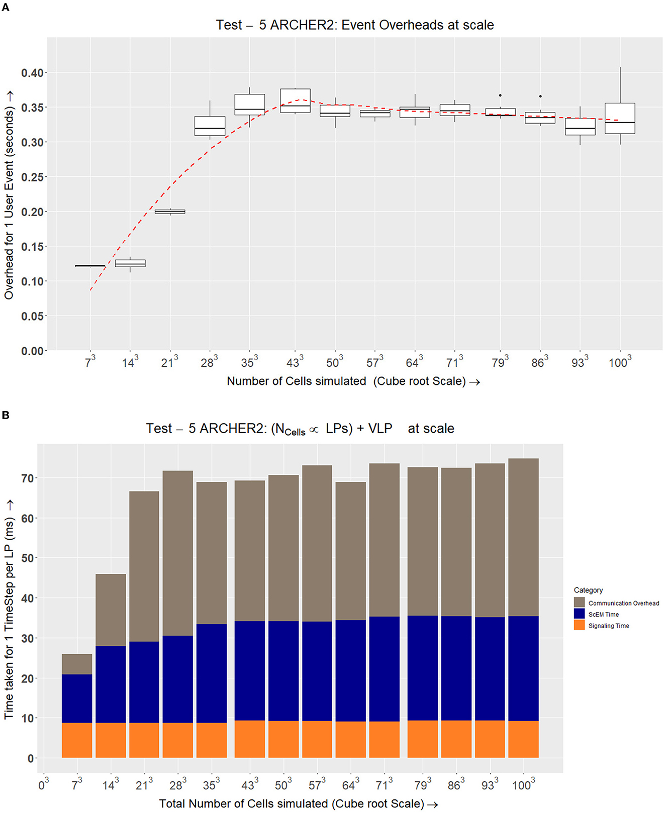
Figure 15. Communication overheads with (A) and without (B) user interactions as we scale up to one million cells. (A) Figures 13B, 14B record the round-trip time between sending a user event and receiving the next set of data from the SLPs. This also includes the amount of time taken between 2 visualizer update intervals. This figure represents the overheads for a user event by subtracting the mean amount of time taken for a visualizer interval without a user-event triggered. (B) The amount of time taken per LP to execute a time-step. This is scaled up until we simulate a total of one million cells. In each case, we are simulating ~40 cells on each LP. Here we can see that in spite of increasing the simulation size, while we add a proportionate number of computational resources, the total amount of time taken remains the same. With the results seen from Figure 8, this simulation can be sped up by using more LPs until each LP hosts a minimum of ~¹/₃^rd of a cell.

In this experiment, we were able to successfully simulate one million cells while verifying their deterministic nature and interacting with the running simulation. The response time is 8 s on ARCHER and 3 seconds on ARCHER2 which, considering the scale of one million cells (over 128 million ScEM agents) is a reasonable time frame to see the effects of a user-defined event on a simulation.

5. Discussion

5.1. Conclusion

The focus of this work is on building a distributed multi-scale framework to simulate large simulations such as cell signaling and physics. The applications of this framework extend to support the development of new cancer drugs and treatment regimes. This simulation will enable domain experts to interactively explore and visualize the effects of different treatments on a simulation of a million-cell spheroid running on local clusters or cloud resources. We draw interactive visualization and simulation techniques from video game technologies and extend their interactivity to HPC environments.

Optimistic synchronization is rarely used in agent-based distributed simulations of complex systems because of the large memory overhead. This paper shows how optimistic synchronization can be used to enable real-time user interaction with a conservatively-synchronized simulation. As the user interactions will be relatively infrequent compared to the complex system interactions, the memory overhead will be minimal.

We ran a distributed cell physics model ScEM (Newman, 2007) with frequent agent-based interactions over ARCHER, an HPC unit using up to 21,953 CPU cores to demonstrate the scalability of this technique. We further developed the simulation by implementing cell-growth, division, and a cell signaling model (Goltsov et al., 2011; Bown et al., 2017) which was deployed on ARCHER2, the successor of ARCHER available at EPCC in Edinburgh (EPCC, 2014), using up to 21,953 CPU cores. The high-speed interconnect in ARCHER2 gives us better performance consistency and reliable results (Section 4).

The message passing density of these applications is much higher than the traditional Parallel Discrete event simulations. In the cell physics model, the state of an agent changes because of the smallest interaction with other agents in the simulation. For instance, if a message is not received in timestep order, an element will be processed wrongly based on its previous state and the positions of its surrounding elements will be incorrect after the forces are applied. This will cascade very quickly across the simulation volume and the overall state of the simulation will be incorrect after very few timesteps.

The forces and communication between agents are similar to other cell physics models (Li, 2015; Ghaffarizadeh et al., 2018). Furthermore, similar implementations of large-scale distributed cell models such as Cytowski and Szymanska (2015, 2014) can easily implement our methods to enable real-time visualization and interactivity.

To show the scalability of the user interaction technique we set out a series of questions in our objectives (Section 1.2). These questions have been revisited and answered below.

(Q1) Does the simulation recover the expected results?One of our key considerations was to maintain the determinism of the complex agent-based system. Regardless of the time taken and scalability, we were able to achieve bit-wise identical results for each experiment that we conducted. This was a result of efficiently utilizing conservative synchronization while avoiding deadlock across different wait points in the simulation. The ordering of floating points made a significant difference in ensuring these files are equal, as without this, round-off accumulation would lead to very different results over time. There are simulation fields that highlight the importance of bit-wise identical results (Liu et al., 2015a,b).

(Q2) Does the simulation scale strongly while keeping the problem-space constant and increasing the LPs?The experimental setup in Test I (Section 4.2) is tailored to answer this question. The results demonstrate that the simulation speeds up well up to a point after which the problem space is too small to compute a meaningful number of agents and the communication overheads surpass the simulation time (see Figure 8). At an optimum size, there needs to be a balance between internal and border agents.

(Q3) Does the simulation scale strongly when we increase the number of LPs with the number of cells?Test II (Section 4.3) showcases that the simulation scales strongly when increasing proportionately to the number of LPs. This is further displayed in Figure 15B where the total amount of time taken by the simulation remains the same when increasing the number of LPs and the cells proportionately.

(Q4) Does the performance change when a visualizer is incorporated?Test III (Section 4.4) showcases that there are no adverse effects of using a visualizer when compared to the same simulation setup in Test II.

(Q5) How long is the round-trip of a user event from the visualizer node?The results from Test V (Section 4.6) record the round trip of a user event on large-scale simulations. The round-trip time of a user event visible to the VLP on our ARCHER2 simulation for 1 million cells (up to 256 million elements) was ≃3s. This is derived from framework parameters that can be adjusted to optimize the visualizer update interval. The round-trip includes the time taken between two visualizer update intervals ΔT_i and the communication overheads of the user events (seen in Figure 15A). The overhead of a response that we observed on ARCHER2 was ~350ms. Comparatively, the user events deployed on SiViT took an average of 1, 409ms for a single cell signaling model in SiViT. In SiViT this time frame was considered acceptable by the domain experts who participated in its evaluation. Our ARCHER2 simulation can further be tweaked to reduce the visualizer update interval and improve the overall round-trip time of a user event. The response time in SiViT would depend on the number of timesteps simulated as SiViT precompiles the simulation data before displaying it to the user. However, our simulation did not observe this limitation as we are interacting with our simulation in real-time.

(Q6) Can the framework simulate a typical cancer spheroid (1 million cells) interactively?At the largest scale, the framework has simulated one million cells effectively. The HPC systems, ARCHER and ARCHER2 used up 21,953 LPs to simulate one million cells which compromise the cell physics and signaling models. Every cell in our physics simulation is composed of sub-cellular elements as described by Newman (2007).

The system works well in a low-latency environment. However, in a high-latency environment, the round-trip latency of a user event will increase proportionately. This work shows that an HPC environment has the infrastructure to execute our communication protocol and respond within a reasonable time frame. Alternatively, when executing this on an uncontrolled LAN cluster, the round-trip time for a user event was approximately 12 s for 256 LPs.

Even though we demonstrate our findings using a cell physics and signaling model, the applications of our user interaction technique are not limited to biomedical simulations such as drug discovery. This technique can be used for other agent-based, high-density complex systems that need to maintain determinism and accuracy such as epidemiology and crowd modeling. Furthermore, the approach can be used for large-scale simulations underpinning Digital Twins; for example, the work conducted by Falconer and Houston (2015) to create a digital twin of soil-microbial complex or urban planning (Isaacs et al., 2011) can be scaled up using this framework in a heterogeneous HPC environment.

Similar large-scale ribosome simulations have been conducted by Sanbonmatsu and Tung (2006) where they simulate up to 2.6 million atoms with a speedup of up to 867. Our simulation in Test I gets a peak speedup of 564 where speedup is T₁/T_LP (Figure 10B). GROMACS (Abraham et al., 2023) is one of the more popular simulation packages available which makes use of MPI for parallel distribution. At present, GROMACS makes use of visualization software such as Rasmol, PyMol, and ChimeraX to view the simulation data after the simulation has been conducted. While the low-level models are different, the simulation architecture used internally by GROMACS is broadly similar to our existing case study, and we believe that it would be practical to adapt it to use our communication algorithms to enable real-time interaction and visualization in molecular dynamics simulations.

5.2. Future work

We envisage this HPC framework to be running on a cloud service while an end-user visualizes and interacts with it in real-time on a local device. Parallelization of ScEM depends primarily on how the latency hiding technique is incorporated. On cloud services, the latency between multiple nodes can be very high as each node is initialized as a virtual machine which adds layers of communication to the MPI-based simulation. As latency hiding in our approach is controllable with the volume of an individual LP (LP), measures can be taken to alter the overall spatial decomposition so that the simulation scales with appropriate cloud computing resources.

An alternative approach to parallelizing ScEM would be utilizing GPU (Graphics processing units) resources over multiple nodes in a cluster. This approach will employ MPI along with a scalable GPU interface such as CUDA (Nickolls et al., 2008) where each MPI process handles a large chunk of the workload and have minimal data transferred between LPs. Using this heterogeneous approach, the force calculations between elements can be sped up; however, with the limited memory available in a GPU, the histories would be stored in the system memory instead. In ScEM, utilizing GPU resources would change the balance between the internal and border elements. This will be a good area for us to explore to speed up this simulation and achieve response times for faster interactions.

Data availability statement

The raw data supporting the conclusions of this article will be made available by the authors, without undue reservation.

Author contributions

NM, AS, and RF contributed to the conception and design of the study. NM and AS wrote the code for the simulations. NM conducted the experiments, gathered the results, and wrote the first draft of the manuscript. AS and RF wrote sections of the manuscript. AB conducted experiments on SiViT and provided additional benchmark data. All authors contributed to the manuscript revision, read, and approved the submitted version.

Acknowledgments

This work was supported by the Northwood Trust. This work used the ARCHER and ARCHER2 UK National Supercomputing Service (https://www.archer2.ac.uk). Financial support for the open access publication fee was provided by Abertay University.

Conflict of interest

The authors declare that the research was conducted in the absence of any commercial or financial relationships that could be construed as a potential conflict of interest.

Publisher's note

All claims expressed in this article are solely those of the authors and do not necessarily represent those of their affiliated organizations, or those of the publisher, the editors and the reviewers. Any product that may be evaluated in this article, or claim that may be made by its manufacturer, is not guaranteed or endorsed by the publisher.

Supplementary material

The Supplementary Material for this article can be found online at: https://www.frontiersin.org/articles/10.3389/fcomp.2023.1085867/full#supplementary-material

References

Abraham, M., Alekseenko, A., Bergh, C., Blau, C., Briand, E., Doijade, M., et al. (2023). GROMACS 2023 Source code. Zenodo. doi: 10.5281/zenodo.7588618

CrossRef Full Text | Google Scholar

Bown, J. L., Shovman, M., Robertson, P., Boiko, A., Goltsov, A., Mullen, P., et al. (2017). A signaling visualization toolkit to support rational design of combination therapies and biomarker discovery: SiViT. Oncotarget 8, 29657–29667. doi: 10.18632/oncotarget.8747

PubMed Abstract | CrossRef Full Text | Google Scholar

Bryant, R. E. (1977). Simulation of Packet Communication Architecture Computer Systems. Technical report MIT/LCS/TR-188, MIT Laboratory for Computer Science.

Google Scholar

Cassandras, C. G. (2008). Introduction to Discrete Event Systems, 2nd Edn. Boston, MA : Springer US.

Google Scholar

Chandy, K. M., and Misra, J. (1979). Distributed simulation: a case study in design and verification of distributed programs. IEEE Trans. Softw. Eng. 5, 440–452.

PubMed Abstract | Google Scholar

Clarke, L., Glendinning, I., and Hempel, R. (1994). “The MPI message passing interface standard,” in Programming Environments for Massively Parallel Distributed Systems, eds K. M. Decker and R. M. Rehmann (Basel: Birkhäuser), 213–218.

Google Scholar

Cordasco, G., Scarano, V., and Spagnuolo, C. (2018). Distributed MASON: a scalable distributed multi-agent simulation environment. Simul. Modell. Pract. Theory 89, 15–34. doi: 10.1016/j.simpat.2018.09.002

CrossRef Full Text | Google Scholar

Cytowski, M., and Szymanska, Z. (2014). Large-scale parallel simulations of 3D cell colony dynamics. Comput. Sci. Eng. 16, 86–95. doi: 10.1109/MCSE.2014.2

CrossRef Full Text | Google Scholar

Cytowski, M., and Szymanska, Z. (2015). Large-scale parallel simulations of 3D cell colony dynamics: the cellular environment. Comput. Sci. Eng. 17, 44–48. doi: 10.1109/MCSE.2015.66

CrossRef Full Text | Google Scholar

Das, S., Fujimoto, R., Panesar, K., Allison, D., and Hybinette, M. (1994). “GTW: a time warp system for shared memory multiprocessors,” in Proceedings of Winter Simulation Conference (Lake Buena Vista, FL), 1332–1339. doi: 10.1109/WSC.1994.717527

CrossRef Full Text | Google Scholar

EPCC (2014). ARCHER Cray XC30. Edinburgh Parallel Computing Centre.

Google Scholar

Falconer, R. E., and Houston, A. N. (2015). Visual simulation of soil-microbial system using GPGPU technology. Computation 3, 58–71. doi: 10.3390/computation3010058

CrossRef Full Text | Google Scholar

Fujimoto, R. M. (1990). Parallel discrete event simulation. Commun. ACM 33, 30–53.

Google Scholar

Ghaffarizadeh, A., Heiland, R., Friedman, S. H., Mumenthaler, S. M., and Macklin, P. (2018). PhysiCell: an open source physics-based cell simulator for 3-D multicellular systems. PLoS Comput. Biol. 14, e1005991. doi: 10.1371/journal.pcbi.1005991

PubMed Abstract | CrossRef Full Text | Google Scholar

Goltsov, A., Faratian, D., Langdon, S. P., Bown, J., Goryanin, I., and Harrison, D. J. (2011). Compensatory effects in the PI3K/PTEN/AKT signaling network following receptor tyrosine kinase inhibition. Cell. Signal. 23, 407–416. doi: 10.1016/j.cellsig.2010.10.011

PubMed Abstract | CrossRef Full Text | Google Scholar

Gutierrez-Milla, A., Borges, F., Suppi, R., and Luque, E. (2014). Individual-oriented model crowd evacuations distributed simulation. Proc. Comput. Sci. 29, 1600–1609. doi: 10.1016/j.procs.2014.05.145

CrossRef Full Text | Google Scholar

Hybinette, M., and Fujimoto, R. M. (2002). Latency hiding with optimistic computations. J. Parallel Distrib. Comput. 62, 427–445. doi: 10.1006/jpdc.2001.1801

CrossRef Full Text | Google Scholar

Isaacs, J. P., Falconer, R. E., Gilmour, D. J., and Blackwood, D. J. (2011). Enhancing urban sustainability using 3D visualisation. Proc. Inst. Civil Eng. Urban Design Plan. 164, 163–173. doi: 10.1680/udap.900034

PubMed Abstract | CrossRef Full Text | Google Scholar

Jefferson, D. R. (1985). Virtual time. ACM Trans. Program. Lang. Syst. 7, 404–425.

Google Scholar

Jefferson, D. R., and Barnes, P. D. (2017). “Virtual time III: unification of conservative and optimistic synchronization in parallel discrete event simulation,” in 2017 Winter Simulation Conference (WSC) (Las Vegas, NV: IEEE), 786–797.

Google Scholar

Kabiri Chimeh, M., Heywood, P., Pennisi, M., Pappalardo, F., and Richmond, P. (2019). Parallelisation strategies for agent based simulation of immune systems. BMC Bioinformatics 20, 579. doi: 10.1186/s12859-019-3181-y

PubMed Abstract | CrossRef Full Text | Google Scholar

Lamport, L. (1978). Time, clocks, and the ordering of events in a distributed system. Commun. ACM 21, 558–565.

Google Scholar

Li, Y. (2015). Agent-based modelling of cell-cell interactions for in vitro vascular formation and cancer cell growth (Ph.D. thesis). Abertay University, Dundee, United Kingdom.

Google Scholar

Liu, L., Li, R., Zhang, C., Yang, G., Wang, B., and Dong, L. (2015a). Enhancement for bitwise identical reproducibility of Earth system modeling on the C-Coupler platform. Geosci. Model Dev. Discuss. 8, 2403–2435. doi: 10.5194/gmdd-8-2403-2015

CrossRef Full Text | Google Scholar

Liu, L., Peng, S., Zhang, C., Li, R., Wang, B., Sun, C., et al. (2015b). Importance of bitwise identical reproducibility in earth system modeling and status report. Geosci. Model Dev. Discuss. 8, 4375–4400. doi: 10.5194/gmdd-8-4375-2015

CrossRef Full Text | Google Scholar

Ma, K. L., and Camp, D. M. (2000). “High performance visualization of time-varying volume data over a wide-area network,” in SC '00: Proceedings of the 2000 ACM/IEEE Conference on Supercomputing, 29. (Dallas, TX). doi: 10.1109/SC.2000.10000

CrossRef Full Text | Google Scholar

Machne, R., Finney, A., Muller, S., Lu, J., Widder, S., and Flamm, C. (2006). The SBML ODE Solver Library: a native API for symbolic and fast numerical analysis of reaction networks. Bioinformatics 22, 1406–1407. doi: 10.1093/bioinformatics/btl086

PubMed Abstract | CrossRef Full Text | Google Scholar

Newman, T. J. (2005). Modeling multicellular systems using subcellular elements. Math. Biosci. Eng. 2, 613–624. doi: 10.3934/mbe.2005.2.613

PubMed Abstract | CrossRef Full Text | Google Scholar

Newman, T. J. (2007). “Modeling multicellular structures using the subcellular element model,” in Single-Cell-Based Models in Biology and Medicine, eds (R. A. Alexander, R. A. Anderson, M. A. J. Chaplain, and K. A. Rejniak), 221–239. doi: 10.1007/978-3-7643-8123-3_10

CrossRef Full Text | Google Scholar

Nickolls, J., Buck, I., Garland, M., and Skadron, K. (2008). Scalable parallel programming with CUDA. Queue 6, 40–53. doi: 10.1145/1365490.1365500

CrossRef Full Text | Google Scholar

Pappalardo, F., Pennisi, M., and Motta, S. (2010). “Universal immune system simulator framework (UISS),” in Proceedings of the First ACM International Conference on Bioinformatics and Computational Biology, BCB '10 (New York, NY: Association for Computing Machinery), 649–650.

Google Scholar

Quan, C. (2014). Network Interconnect Evaluation on ARCHER, University of Edinburgh.

Google Scholar

Rapaport, D. C. (2004). The Art of Molecular Dynamics Simulation, 2 Edn. Cambridge: Cambridge University Press.

Google Scholar

Rousset, A., Herrmann, B., Lang, C., and Philippe, L. (2015). “A communication schema for parallel and distributed multi-agent systems based on MPI,” in Euro-Par 2015: Parallel Processing Workshops, eds S. Hunold, A. Costan, D. Gimenez, A. Iosup, L. Ricci, M. E. Gomez Requena, V. Scarano, A. L. Varbanescu, S. L. Scott, S. Lankes, J. Weidendorfer, and M. Alexander (Cham: Springer International Publishing), 442–453.

Google Scholar

Sanbonmatsu, K. Y., and Tung, C.-S. (2006). Large-scale simulations of the ribosome: a new landmark in computational biology. J. Phys. Conf. Ser. 46, 334. doi: 10.1088/1742-6596/46/1/047

PubMed Abstract | CrossRef Full Text | Google Scholar

Schroeder, W. J., Martin, K. W., and Lorensen, B. (2006). The Visualization Toolkit, 4th Edn. Clifton Park, NY: Kitware.

Google Scholar

Shen, W., Lu, W., Wei, D., Xu, W., Zhu, X., and Yuan, S. (2009). “A parallel algorithm for computer simulation of electrocardiogram based on MPI,” in 2009 Eighth IEEE/ACIS International Conference on Computer and Information Science (Shanghai), 120–123. doi: 10.1109/ICIS.2009.110

PubMed Abstract | CrossRef Full Text | Google Scholar

Smith, A., and Narula, H. (2017). Improbable Solving Problems and Building Worlds with SpatialOS @GDC '17. Available online at: https://www.youtube.com/watch?v=_X-NBGSmE6c

Google Scholar

Somogyi, E. T., Bouteiller, J.-M., Glazier, J. A., Konig, M., Medley, J. K., Swat, M. H., et al. (2015). libRoadRunner: a high performance SBML simulation and analysis library. Bioinformatics 31, 3315–3321. doi: 10.1093/bioinformatics/btv363

PubMed Abstract | CrossRef Full Text | Google Scholar

Van Liedekerke, P., Palm, M. M., Jagiella, N., and Drasdo, D. (2015). Simulating tissue mechanics with agent-based models: concepts, perspectives and some novel results. Comput. Particle Mech. 2, 401–444. doi: 10.1007/s40571-015-0082-3

CrossRef Full Text | Google Scholar