Device Classification for Industrial Control Systems Using Predicted Traffic Features

To achieve a secure interconnected Industrial Control System (ICS) architecture, security practitioners depend on accurate identification of network host behavior. However, accurate machine learning based host identification methods depends on the availability of significant quantities of network traffic data, which can be difficult to obtain due to system constraints such as network security, data confidentiality, and physical location. In this work, we propose a network traffic feature prediction method based on a generative model, which achieves high host identification accuracy. Furthermore, we develop a joint training algorithm to improve host identification performance compared to separate training of the generative model and the classifier responsible for host identification.

1. Introduction

Modern Industrial Control Systems (ICS) carry out the automation of industrial processes via complex, interconnected, large-scale arrangements of sensors, actuators, and specialized and general-purpose computing devices. As high-visibility ICS cyber-security events over the past two decades have shown, left unsecured, these cyber-physical systems can be vulnerable to misuse and abuse, leading to real-world consequences. A first step toward securing internetworked cyber-physical ICS is to identify, or characterize the network hosts so that an informed security posture assessment can be performed. Conventional Information Technology (IT) tools often use human-specified rules, signatures, and fingerprints to characterize network hosts, and these techniques have been adapted to ICS networks. These conventional characterization techniques begin to break down in ICS environments due to the breadth of device types and specialized communication protocols used in ICS networks; maintenance of databases used by conventional techniques need to be continuously updated to keep up with the introduction of new device types, operating systems and communication protocols. Due to the essential nature of critical infrastructure and ICS for society at large, and the possibility of accurate and high-performance automation of security-related tasks, such as the determination of device characteristics like model and manufacturer, much work has been done recently in the field of Machine Learning (ML) to devise methods of characterizing network hosts, and specifically, ICS devices, so as to avoid much of the downsides of conventional host characterization techniques.

Previous work shows the effectiveness of both network traffic features and ICS protocol features for ICS network device classification (Chakraborty et al., 2021). However, in order to acquire such features, it is necessary to capture network traffic data from the relevant ICS network and then perform network-packet level analysis on that data. This is a non-trivial undertaking, especially in ICS networks which may be physically isolated and difficult to access, resource constrained (e.g., in network bandwidth and storage), or where access is restricted due to confidentiality concerns. In such an environment, we may have access to a limited amount of network traffic data. The objective of this work is to augment the collection of real ICS network data with a computationally inexpensive process, which can generate realistic traffic features as a function of time.

In this work, we frame the above as a time-series forecasting problem and seek to answer two questions: (1) Given a partial history of network traffic, can we accurately forecast that history into the future? and (2) Can we use this network traffic forecast to improve device classification performance? To answer these questions, we develop and evaluate a novel approach comprised of two key elements: (1) a time-series forecasting model based on a sequence-to-sequence (Seq2Seq) deep learning architecture and (2) a joint training procedure for the Seq2Seq model and the device classifier, in which the Seq2Seq model functions as a traffic feature generator and the classifier functions as a data discriminator, implicitly evaluating the quality of the traffic features generated by the Seq2Seq model. We demonstrate that these two pieces are both necessary and sufficient to significantly improve device classification performance (up to a 23% increase in accuracy) in a data-constrained ICS setting.

1.1. Main Contribution

We highlight the main contribution of this work, before getting into the technical details.

• The primary contribution of this work is the development of a novel machine learning framework, which jointly trains (a) a network traffic forecasting model and (b) a traffic-feature based device classification model, and which produces significant improvements in device classification performance over a similar approach with independently trained model components.

• This proposed framework is shown to be useful in a data-constrained scenario, which is common for ICS due to network security, as shown in Figure 1.

FIGURE 1

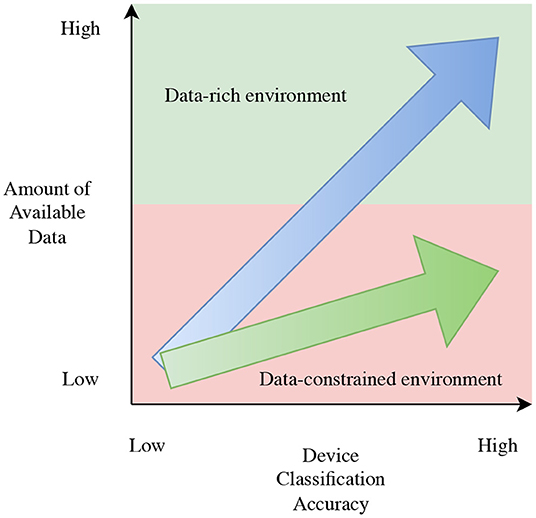
Figure 1. The accuracy of ICS device classification methods depends on the amount of available data (blue arrow). In data-constrained environments, classification accuracy may suffer. The goal of this work is to develop methods to reduce the slope of the data-accuracy relation such that higher ICS device classification accuracy may be obtained with less data (green arrow).

2. Related Work

Time series modeling has historically been a key area of academic research, forming an integral part of applications in topics such as climate modeling (Mudelsee, 2019), biological sciences (Stoffer and Ombao, 2012), and medicine (Topol, 2019), as well as commercial decision making in retail (Böse et al., 2017), finance (Andersen et al., 2005), and net-load consumption for customer (Thayer et al., 2020) to name a few. While traditional methods have focused on parametric models informed by domain expertise such as autoregressive (AR) (Box and Jenkins, 1976), exponential smoothing (Winters, 1960; Gardner, 1985), or structural time series models (Harvey, 1990), modern machine learning methods provide a means to learn temporal dynamics in a purely data-driven manner (Ahmed et al., 2010). With the increasing data availability and computing power in recent times, machine learning has become a vital part of the next generation of time series forecasting models.

Deep learning in particular has gained popularity in recent times, inspired by notable achievements in image classification (Krizhevsky et al., 2012), natural language processing (Devlin et al., 2018), and reinforcement learning (Silver et al., 2016). By incorporating bespoke architectural assumptions, inductive biases (Baxter, 2000), that reflect the nuances of underlying datasets, deep neural networks are able to learn complex data representations (Bengio et al., 2013), which alleviates the need for manual feature engineering and model design. The availability of open-source backpropagation frameworks (Abadi et al., 2016; Paszke et al., 2019) has also simplified the network training, allowing for the customization for network components and loss functions.

Given the diversity of time-series problems across various domains, numerous neural network design choices have emerged. A rich body of literature exists for automated approaches to time series forecasting including automatic parametric model selection (Hyndman and Khandakar, 2008), and traditional machine learning methods such as kernel regression (Nadaraya, 1964) and support vector regression (Smola and Schölkopf, 2004a). In addition, Gaussian processes (Williams and Rasmussen, 1996) have been extensively used for time series prediction with recent extensions including deep Gaussian processes (Damianou and Lawrence, 2013), and parallels in deep learning via neural processes (Garnelo et al., 2018). Furthermore, older models of neural networks have been used historically in time series applications, as seen in Waibel (1989) and Wan (1993).

In the domain of Information Technology communication networks, traffic forecasting and prediction is an active area of research. While the literature uses the terms somewhat interchangeably, strictly speaking, forecasting is the task of using a model to estimate the future value of a variable (such as number of bytes transferred, for example) based on previous, time-ordered values of the same variable, while prediction uses a model to estimate the value of an unknown variable based on the values of other known variables. Thus, forecasting is a sub-discipline of prediction that focuses on time. Historical and modern uses of traffic forecasting include trunk demand servicing, planning for network design and capacity upgrade requirements, network control, bandwidth provisioning, and efficient resource utilization. Early work focused primarily on the application of Kalman filters, the Sequential Projection Algorithm (SPA), and Autoregressive Integrated Moving Average (ARIMA) models to predict traffic behavior of telecommunication networks and Internet forerunners (Szelag, 1982; Groschwitz and Polyzos, 1994).

Subsequent work continued to apply ARIMA model variants to modern Internet traffic and mobile wireless networks while improving the prediction time-step resolution (Shu et al., 1999; Liang, 2002; Papagiannaki et al., 2003, 2005; El Hag and Sharif, 2007). Simultaneously, new methods based on Autoregressive Conditional Heteroskedasticity (ARCH) models were introduced (Krithikaivasan et al., 2007; Kim, 2011) to capture the observed second-order non-stationarity of real traffic data.

Artificial Intelligence and Machine Learning methods for predicting communication network traffic gained popularity in the 2000's with the successful application of fuzzy logic and artificial neural network models (Liang, 2002; Guang et al., 2004). A large volume of AI and ML work for predicting traffic appeared in the following decades, and we refer the reader to surveys of ML applications to traffic forecasting and traffic characterization (Mohammed et al., 2019; Xie et al., 2019), as applied to Software Defined Networks in particular, for more detailed discussions.

In this article, we present a classification problem based on predicted time series data. For an ICS dataset, availability of sufficient network data significantly affects the classification accuracy for classifying ICS and non-ICS devices, as shown in Chakraborty et al. (2021). This motivates the requirement of defining a time series prediction task, associated with a classification task using the predicted time series data. Therefore, our proposed method lies in the intersection of regression and prediction tasks.

2.1. Paper Structure

The remainder of this article is structured as follows: in Section 3 we describe the ICS dataset used for this work; in Section 4 we formally introduce the problem solved in this work; in Section 5 we introduce the method used for the time series prediction and in Section 6 we develop the model used for the prediction task; in Section 7 we describe the results while using the prediction model for the classification task; and finally, in Section 8, we discuss findings of our current work.

3. Data Description

Network flows from a production-level industrial electrical distribution system (Site A) are utilized for this work. First, (TCP and UDP) network flow datasets were generated for this system by processing passively captured network traffic in PCAP form. Based on the source port of the network flows, the flows are categorized into ICS and non-ICS flows.

Network traffic for Site A is attributed to one of six different protocol groups: ARP, TCP/IP, DNP3 (Distributed Network Protocol, version 3), HTTP, TLS, and UDP. Before calculating the traffic features, the packets within each flow are subdivided according to these protocol types. Ten standard traffic features, shown in Table 1, are selected for this flow classification task. These traffic features are then computed for the extracted traffic flows for Site A. Since the captured data from Site A is not large enough to achieve sufficient device classification accuracy, our objective is to forecast (predict) the traffic features listed in Table 1 using the measured flows from Site A, which then can be used to perform the flow classification task with expectantly higher accuracy¹.

TABLE 1

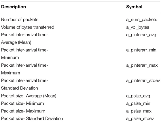
Table 1. Feature list per protocol, per direction. In the “Symbol” column “a” is either sent or received, representing each direction of flow.

To illustrate the observed characteristics of the Site A traffic features, Figure 2 plots 10, 000 timesteps (with each timestep having a resolution of 10 s, for a total of 100, 000 s) of each feature for sent and received packets, for both ICS and non-ICS devices. Four different colors in Figure 2 indicate the sent and received traffic features associated with ICS and non-ICS traffic flows.

FIGURE 2

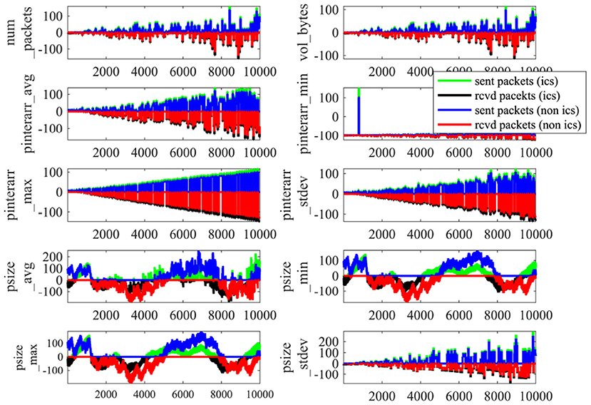
Figure 2. Snapshot of the time series measurement of features associated with Site A.

4. Problem Formulation

Consider a dataset consisting of traffic features, ${D}$_t, is present for Site A with ICS and non-ICS devices. This dataset can be utilized to identify the device types (ICS or non-ICS, and device manufacturer and model number), as demonstrated in Chakraborty et al. (2021). Furthermore, we assume the length of the collected dataset, t, is less than the optimal data length (T) required for obtaining a desired device classification accuracy, as shown in Section 4 of Chakraborty et al. (2021). Now we formally define the two problem statements.

Problem 1 (Prediction model). Given a traffic feature dataset of time length t, and an optimal data length requirement of T, can we develop a prediction model for forecasting the traffic features from time t to time T?

Problem 2 (Classification using prediction model). Using the prediction model from Problem 1, can we get the desired device classification accuracy for Site A?

5. Time-Series Prediction Methodology

One of the primary tasks associated with solving Problem 1 and Problem 2 is obtaining a sufficiently accurate² prediction of traffic features for ICS and non-ICS traffic. We propose a sequence-to-sequence model (Seq2Seq) based deep network architecture for the time series prediction task. The Seq2Seq model (Sutskever et al., 2014) is comprised of a Long Short Term Memory (LSTM, Hochreiter and Schmidhuber, 1997) based encoder-decoder.

5.1. Seq2Seq Model

We used a sequence-to-sequence model architecture as shown in Figure 3 with context based encoding-decoding as in Luong et al. (2015). Here we repeat some important aspects of the Luong context-based Seq2Seq architecture, as we refer to aspects of this architecture that were tuned for our application in Section 6.4.

FIGURE 3

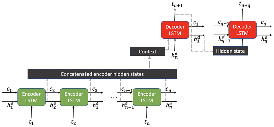
Figure 3. Schematic of Luong et al. (2015) context based Seq2Seq architecture.

Let $\text{E}\triangleq \left\{h_1^e,h_2^e,\dots ,h_n^e\right\}$ represent the hidden states of the n encoder units and $\text{D}\triangleq \left\{h_1^d,h_2^d\dots ,h_q^d\right\}$ represent the hidden states of the q decoder units of a Seq2Seq model, where each $h_i^{*}\in {\text{R}}^{h\times 1}$ comes from a LSTM unit. The prediction at each decoder is calculated as defined below.

$\begin{array}{l}{h}_i^d=f(h_{i-1}^d,{ŷ}_{i-1}),\\ {\alpha }_{i*}=\text{score}(h_i^d,E),\\ {\bar{\alpha }}_{i*}=\text{Softmax}({\alpha }_{i*}),\\ c_i={\displaystyle \sum _{j=1}^l}{\bar{\alpha }}_{ij}{h}_j^e,\\ {\tilde{h}}_i^d=\text{tanh}({\text{W}}_h\star \left[c_i;h_i^d\right]),\\ {ŷ}_i=g({\tilde{h}}_i^d).& (1)\end{array}$

In Equation (1), f is a recurrent unit like a LSTM, $h_{i-1}^d$ represents the hidden state from the previous decoder unit and ${ŷ}_{i-1}\in {ℝ}^{k\times 1}$ is the k-variate prediction of the previous decoder unit passed as input to the current decoder unit. ${\bar{\alpha }}_{i\star }\in {ℝ}^{l\times 1}$ is the attention weight vector for decoder i over the encoder hidden states (i.e., l = ||E||) and $c_i\in {ℝ}^{h\times 1}$ is the attention context vector calculated as a linear combination over all E, and corresponding attention weights ${\bar{\alpha }}_{i\star }$.

The attention energy vector α_i⋆ for the i-th decoder unit can be calculated in multiple ways. The attention energies can be calculated purely based on the current hidden vector or as a function of the alignment between the current hidden vector and encoder states, as shown in Equation (2).

$\begin{array}{ll}score(h_i^d,E)={\text{W}}_{\alpha }{h}_i& (2)\end{array}$

The attention energies are then normalized using a softmax transformation, to obtain the attention weights ${\bar{\alpha }}_{i*}\in {ℝ}^{l\times 1}$, which is then used to obtain the attention context vector c_i.

Next, the attention hidden state ${\tilde{h}}_i^d$ of the i-th decoder is obtained by imposing a nonlinear transfer function (hyperbolic tangent) over an affine transformation (with ${\text{W}}_h\in {ℝ}^{h\times 2h}$) of the concatenation of c_i and $h_i^d$. Finally, g is a function which calculates the i-th prediction ŷ_i from the corresponding decoder attention hidden state ${\tilde{h}}_i^d$i. For this case, we consider g to be a linear function. In Figure 3, a schematic of the proposed Seq2Seq architecture is shown.

6. Prediction Model Development

In this section we will utilize the Seq2Seq architecture mentioned in Section 5.1 to solve Problem 1. Before describing the solution results, we briefly describe the data processing step and the evaluation metrics for the time series prediction.

6.1. Data Generation

The network flow data contains packet level information between different devices present in the dataset. We have extracted different traffic features (as listed in Table 1) across specific type of device (in both sending and receiving direction). Therefore from the network flow data, we extract time series measurement of different traffic features across individual present devices. We have collected the network flow data for a pre-defined amount of time. In Section 6.5, for brevity we evaluated our prediction model for predicting ICS and Non-ICS flows (average of all the traffic features for the broader class of ICS and Non-ICS devices), however in Section 7, we evaluated the time series prediction performance for individual devices. In this whole section, the experimental setup is as described in Problem 1, with t = 12, 000 and T = 16, 000, unless explicitly mentioned otherwise.

6.2. Data Processing

For the prediction task, we extracted the trend lines using “scikit-learn”-SVR (support vector regression) package, from the time series measurements for both ICS and non-ICS flows. As shown in Figure 4, the blue and red solid lines show the total number of transferred packets for ICS and non-ICS flows, respectively. In Figure 4, the black lines show the trend line for both type of flows. For the prediction task, the proposed architecture will be evaluated for the “detrend” line, as shown in the zoomed-box in Figure 4. The “detrend” line is calculated by subtracting the trend line from the traffic feature measurements.

FIGURE 4

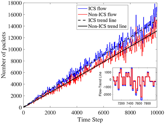
Figure 4. Total number of transferred packets for ICS and non-ICS devices vs. time. Trend lines for both time series are shown as dashed and solid lines for ICS and non-ICS devices, respectively. The inset shows the time series “detrended,” i.e., the trend lines subtracted from the original time series.

6.3. Evaluation Metrics

Table 2 describes the metrics used to evaluate the performance of the proposed Seq2Seq model architecture.

TABLE 2

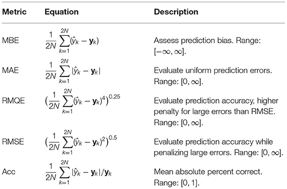
Table 2. Evaluation metrics for the ICS and non-ICS traffic feature prediction architecture.

6.4. Seq2Seq Model Exploration

In this section, we will evaluate the effect that different architecture hyperparameters (number of hidden neurons of the LSTM layer, input sequence length, i.e., input data dimension, output sequence length, i.e., output data dimension) have on ICS and non-ICS sequence prediction performance. We used standard k-folding, with k = 100 (160 time points in each fold), for evaluating the performance of different hyperparameter values, using the evaluation metrics introduced in Section 6.3.

As shown in Figure 5, we varied the number of LSTM neurons (dimension h as introduced in Section 5.1) of the Seq2Seq model between 20 and 190, with an increment of 10, and plotted the evaluation metrics (Figure 5, all the evaluation metrics are calculated as an average over all the traffic features). As shown in Figure 5, with an increase in the number of hidden neurons, all the evaluation metrics improve, although there is a parabolic increase in the number of trainable parameters. Therefore, for the sake of the burden of computational complexity, we have selected 100 hidden neurons for our Seq2Seq model architecture for future performance evaluation.

FIGURE 5

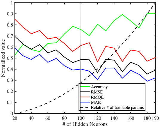
Figure 5. Variation of the evaluation metrics (averaged over the extracted features) with the number of LSTM hidden neurons. The black vertical line is the number of neurons we selected for our architecture.

We also evaluated the prediction performance of the proposed Seq2Seq model, by varying the input sequence length (number of input data points at each step, i.e., number of encoder units n as introduced in Section 5.1). As shown in Figure 6, the evaluation metrics are plotted while varying the input sequence length between 40 and 380 (as before, all the evaluation metrics are calculated as an average over all the traffic features). Figure 6 shows that MAXE improves while increasing n between 40 and 180, and stays almost unchanged thereafter, while the other three metrics remain unchanged while varying n. This shows that the effect of increasing input sequence length does not affect the prediction performance. Therefore, we have selected 200 encoder units for our Seq2Seq model architecture for future performance evaluation.

FIGURE 6

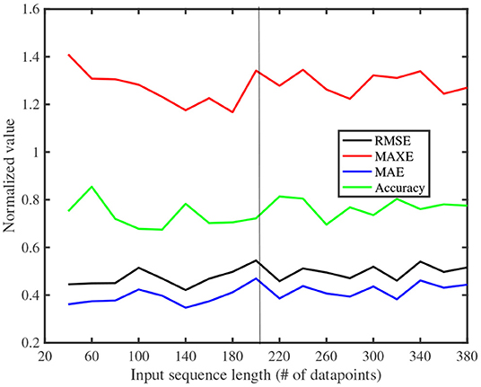
Figure 6. Variation of the evaluation metrics with input sequence length. The black vertical line is the selected input sequence length for our proposed architecture.

Finally, the prediction performance of the proposed Seq2Seq model is evaluated by varying the output sequence length (number of output time step, i.e., number of decoder units q as introduced in Section 5.1). As before, four evaluation metrics were computed while varying q between 30 and 1, 000. All the evaluation metrics degrade while increasing the output prediction sequence length as shown in Figure 7. Note that, for this evaluation, the aforementioned model parameters are kept constant at the selected value. Therefore, we have selected 30 decoder units for our Seq2Seq model architecture for future performance evaluation.

FIGURE 7

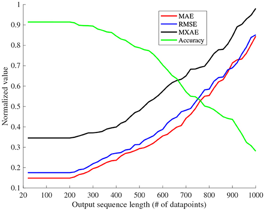
Figure 7. Variation of the evaluation metrics with the output sequence length (prediction length). The black vertical line is the selected output sequence length for our architecture.

For further clarity, we have put the detailed parameter values of Seq2Seq model, in Table 3.

TABLE 3

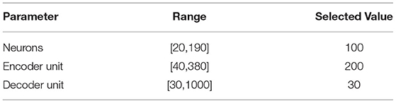
Table 3. Parameter list and the selected values for the Seq2Seq model.

6.5. Performance Comparison of ICS and Non-ics Traffic Features

In this section, we evaluate the prediction performance between ICS and non-ICS traffic features. In Figure 8, we calculated the percentage of prediction error³ and plotted the histogram variation with different traffic features. The features are in the same order as they appear in Table 1. Therefore, features 1 to 10 are for ICS flows and 11 to 20 are for non-ICS flows. For both ICS and non-ICS traffic flows, the prediction performance is better for maximum and standard deviation values of packet inter-arrival time, compared with the other eight features. It is important to note here that using the recursive feature elimination (RFE, Guyon et al., 2002) algorithm, in the context of device classification, our prediction model performs better for predicting the highest ranked traffic features, such as packet inter-arrival time.

FIGURE 8

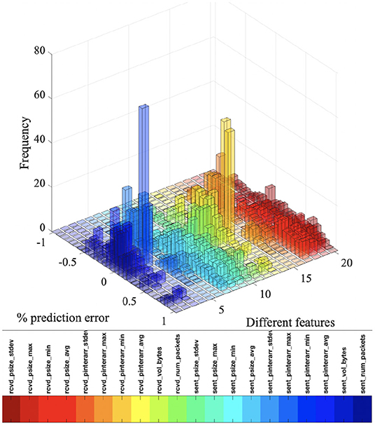
Figure 8. Histogram plot of percentage of prediction error variation with different traffic features.

6.6. Time Series Comparison

In this section we plot time series measurements and their prediction for the test dataset. Figures 9, 10 show the overlapped time series plots of the true value and the predicted value for ICS and non-ICS traffic features. The Seq2Seq architecture performs better in predicting all of the traffic features, except for the one associated with packet size. Even for the packet size related features (which vary the most with time), our proposed architecture performs significantly well.

FIGURE 9

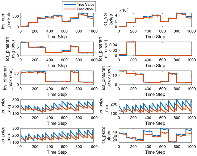
Figure 9. Time series plots of the true and predicted values for ICS traffic features. We have plotted the first 1, 000 data points out of predicted 4, 000, for visual clarity.

FIGURE 10

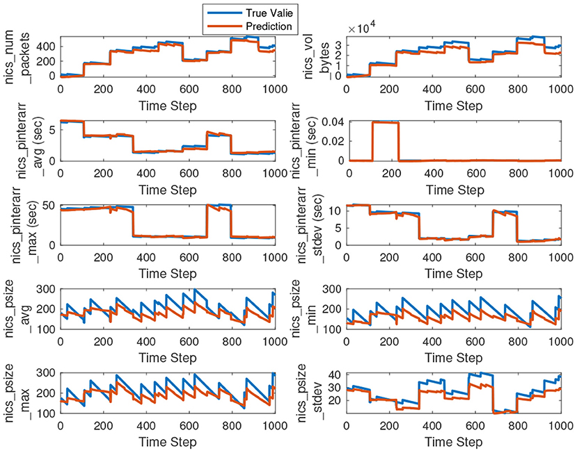
Figure 10. Time series plots of the true and predicted values for non-ICS traffic features. We have plotted the first 1, 000 data points out of predicted 4, 000, for visual clarity.

6.7. Performance Comparison With Other Methods

In this section, we perform comparisons with other contemporary machine learning models present in the existing literature. Specifically, we compare the proposed Seq2Seq model's performance with Multilayer Perceptron (MLP) (Rosenblatt, 1961), Linear Regression (LR) (Bianco et al., 2009), Linear Support Vector Regression (LSVR) (Smola and Schölkopf, 2004b), Random Forest (RF) (Hedén, 2016), and Gaussian Mixture model (Srivastav et al., 2013). We evaluated the prediction performance of these methods for our dataset, presented in Figure 11. We observe that the Seq2Seq model outperforms all of the aforementioned machine learning methods in all performance categories.

FIGURE 11

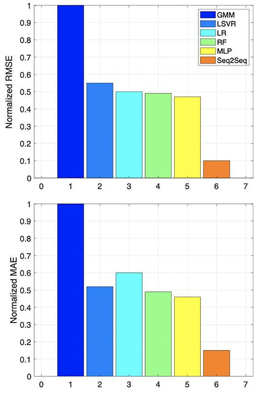
Figure 11. Performance comparison of the Seq2seq model with existing methods. The top plot shows the normalized RMSE, and the bottom plot shows the normalized MAE.

Furthermore, we compare the performance of the proposed Seq2Seq model with three different loss functions (weighted combination of mean absolute error (MAE), Kullback-Leibler divergence (KL), and Maximum absolute error (Max), and the Dilated ConvNet (Yazdanbakhsh and Dick, 2019). As shown in Figure 12, for different traffic features, the Seq2Seq model with the combination loss function of (10*MAE+KL+Max) performs better than other deep network architectures.

FIGURE 12

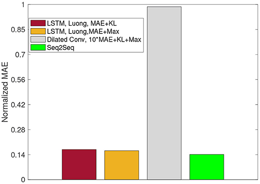
Figure 12. MAE variation averaged over all traffic features for different deep network architectures.

7. Classification Using the Seq2Seq Prediction Model

Device classification requires measured data from Site A of at least time length T for satisfactory classification performance (Chakraborty et al., 2021). For our dataset, using the optimal time length calculation, we have evaluated the required length to be 16, 000 data points for achieving overall classification accuracy more than 90% across all present devices. However, suppose that only 12, 000 data points of measured data from Site A are available, leading to reduced classification performance. We propose to use an additional 4, 000 time steps of predicted data to improve the performance of the classification task.

As proposed in Chakraborty et al. (2021), we used the traffic features as features for classifying various devices present in Site A. Before showing the performance of our prediction model in this context, we define our baseline performance as the device classification performance with 12, 000 measured data points. As seen in Figure 13, the confusion matrix shows the classification performance for six devices, with all available measurement data. We further note that we can achieve an overall classification accuracy of 73.62%, where “Workstation” and “Server” are misclassified most often. Similarly, misclassification is also noted between SEL devices.

FIGURE 13

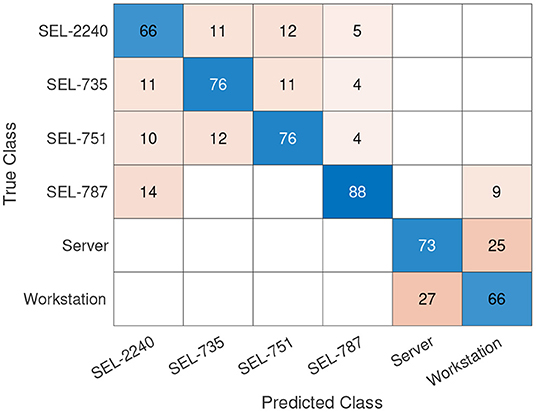
Figure 13. Confusion matrix with 12000 data points of measured data. The classification dataset is unbalanced with a class ratio of 17:21:2:1:12:2 (the class ratio has the same order as the confusion matrix).

Now, as previously proposed, we added 4, 000 data points from our prediction model, along with the present 12, 000 measurement data points. Then, these 16, 000 data points of traffic features are used as feature vectors for classifying the same six devices. Similar to Figures 13, 14 shows the updated confusion matrix for the device classification task. Although we have added more data points to our feature set, we do not see any significant classification performance increase when compared to the baseline result. More precisely, SEL-735, SEL-751, and SEL-787 classification performance was improved on average over 15%, however the classifier shows a performance reduction of 10% for SEL-2240, with the new dataset.

FIGURE 14

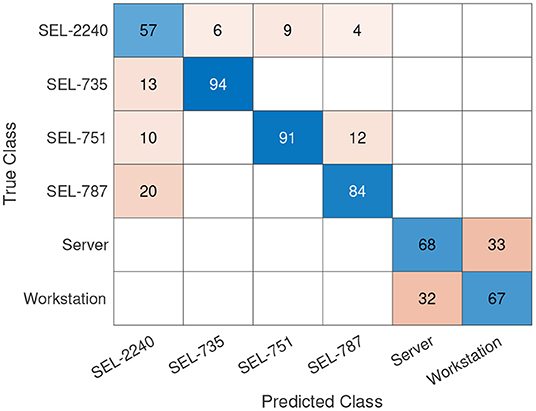
Figure 14. Confusion matrix with 12, 000 data points of measured data and 4, 000 data points of predicted data with separate training of Seq2Seq model and the classifier. The classification dataset is unbalanced with a class ratio of 17:21:2:1:12:2 (the class ratio has the same order as the confusion matrix).

Next, we propose to train the Seq2Seq model and the classifier with a combined loss function to improve the device classification accuracy.

7.1. Combined Training of Seq2Seq Model and Classifier

We propose to improve the device classification performance shown in Figure 14, by a joint training of the Seq2Seq model and the classifier. The Seq2Seq model works as a traffic feature generator, while the classifier responsible for device classification works as a data discriminator, evaluating the quality of the traffic features generated from the Seq2Seq model. For demonstration, we adopt the notation similar to Arora et al. (2017) and Li et al. (2018). Let ${G}$ = G_g, g∈${U}$ and ${D}$ = D_d, d∈${V}$ denote the Seq2Seq model based traffic feature generator and device classification based discriminator respectively, where G_g and D_d are functions parameterized by g and d. ${U}$, ${V}$⊆ℝ^p represents the respective parameter spaces of the generator and discriminator. Finally, let G^* be the target known distribution to which we would like to fit our Seq2Seq model, which utilizes the measured 12000 data points. We incorporate a combined weighted loss of regression and classification for the combined training of ${G}$ and ${D}$. We found a weight ratio of 1:10, for regression to classification, works best for optimum classification performance; this was determined by experimental variation of the weight ratio.

To compare performance with Figure 14, we generated the same amount of predicted data as in Figure 14, using the combined loss function training. The classification performance is shown in Figure 15, which shows an overall increase in classification accuracy of around 15%, across all devices. Particularly, we can see a classification accuracy improvement of over 23% for “Workstation” and “Server” device types. The traffic feature prediction using this combination loss function performs significantly better compared to both the separate training (Figure 14) and the baseline (Figure 13).

FIGURE 15

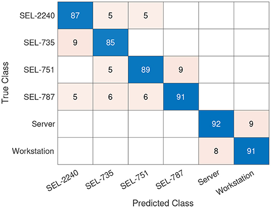
Figure 15. Confusion matrix with 12, 000 data points of measured data and 4, 000 data points of predicted data with combined training of the Seq2Seq and the classifier. The classification dataset is unbalanced with a class ratio of 17:21:2:1:12:2 (the class ratio has the same order as the confusion matrix).

8. Conclusion

ICS device classification requires a minimum amount of collected traffic flow data for satisfactory classification performance. Due to various constraints, we do not always have access to the required amount of data and therefore we propose an alternative approach of device classification. Our proposed approach utilizes a Seq2Seq based deep network architecture for traffic feature prediction, related to device classification. Moreover, a classifier responsible for identifying device types is used to evaluate the quality of the predicted data. We further show that a combined training of a prediction model and a classifier improves the device classification performance by as much as 23%, compared to separate training.

Data Availability Statement

The datasets presented in this article are not readily available because, the data is generated for the sole purpose of internal research effort. Requests to access the datasets should be directed to kelley35@llnl.gov.

Author Contributions

IC, BK, and BG: study conception and design and draft manuscript preparation. BK: data collection. IC: analysis and interpretation of results. All authors reviewed the results and approved the final version of the manuscript.

Funding

This work was performed under the auspices of the U.S. Department of Energy by Lawrence Livermore National Laboratory under Contract DE-AC52-07NA27344 and was supported by the LLNL-LDRD Program under Project No. 19-ERD-021.

Conflict of Interest

The authors declare that the research was conducted in the absence of any commercial or financial relationships that could be construed as a potential conflict of interest.

Publisher's Note

All claims expressed in this article are solely those of the authors and do not necessarily represent those of their affiliated organizations, or those of the publisher, the editors and the reviewers. Any product that may be evaluated in this article, or claim that may be made by its manufacturer, is not guaranteed or endorsed by the publisher.

Footnotes

1. ^We have shown in Chakraborty et al. (2021) that a minimum amount of data is required to achieve a specific ICS device classification accuracy.

2. ^Prediction accuracy is defined in the literature (Thayer et al., 2020) based on several performance metrics, such as root mean square error, mean bias error etc.

3. ^100 × (true value-prediction value)/true value.

References

Abadi, M., Agarwal, A., Barham, P., Brevdo, E., Chen, Z., Citro, C., et al. (2016). Tensorflow: Large-scale machine learning on heterogeneous distributed systems. arXiv [Preprint] arXiv:1603.04467.

Google Scholar

Ahmed, N. K., Atiya, A. F., Gayar, N. E., and El-Shishiny, H. (2010). An empirical comparison of machine learning models for time series forecasting. Econ. Rev. 29, 594–621. doi: 10.1080/07474938.2010.481556

CrossRef Full Text | Google Scholar

Andersen, T. G., Bollerslev, T., Christoffersen, P. F., and Diebold, F. X. (2005). Volatility Forecasting. Technical report, National Bureau of Economic Research. doi: 10.3386/w11188

CrossRef Full Text | Google Scholar

Arora, S., Ge, R., Liang, Y., Ma, T., and Zhang, Y. (2017). “Generalization and equilibrium in generative adversarial nets (GANs),” in International Conference on Machine Learning, 224–232.

Google Scholar

Baxter, J. (2000). A model of inductive bias learning. J. Artif. Intell. Res. 12, 149–198. doi: 10.1613/jair.731

CrossRef Full Text | Google Scholar

Bengio, Y., Courville, A., and Vincent, P. (2013). Representation learning: a review and new perspectives. IEEE Trans. Pattern Anal. Mach. Intell. 35, 1798–1828. doi: 10.1109/TPAMI.2013.50

PubMed Abstract | CrossRef Full Text | Google Scholar

Bianco, V., Manca, O., and Nardini, S. (2009). Electricity consumption forecasting in Italy using linear regression models. Energy 34, 1413–1421. doi: 10.1016/j.energy.2009.06.034

CrossRef Full Text | Google Scholar

Böse, J.-H., Flunkert, V., Gasthaus, J., Januschowski, T., Lange, D., Salinas, D., et al. (2017). Probabilistic demand forecasting at scale. Proc. VLDB Endow. 10, 1694–1705. doi: 10.14778/3137765.3137775

CrossRef Full Text | Google Scholar

Box, G. E., and Jenkins, G. M. (1976). Time Series Analysis: Forecasting and Control San Francisco. San Francisco, CA: Holden-Day.

Google Scholar

Chakraborty, I., Kelley, B. M., and Gallagher, B. (2021). Industrial control system device classification using network traffic features and neural network embeddings. Array 12:100081. doi: 10.1016/j.array.2021.100081

CrossRef Full Text | Google Scholar

Damianou, A., and Lawrence, N. D. (2013). “Deep gaussian processes,” in Artificial Intelligence and Statistics, 207–215.

Google Scholar

Devlin, J., Chang, M.-W., Lee, K., and Toutanova, K. (2018). Bert: pre-training of deep bidirectional transformers for language understanding. arXiv [Preprint] arXiv:1810.04805.

Google Scholar

El Hag H. M. A. and Sharif, S. M. (2007). “An adjusted ARIMA model for internet traffic,” in AFRICON 2007 (Windhoek), 1–6. doi: 10.1109/AFRCON.2007.4401554

CrossRef Full Text | Google Scholar

Gardner, E. S. Jr. (1985). Exponential smoothing: the state of the art. J. Forecast. 4, 1–28. doi: 10.1002/for.3980040103

CrossRef Full Text | Google Scholar

Garnelo, M., Rosenbaum, D., Maddison, C., Ramalho, T., Saxton, D., Shanahan, M., et al. (2018). “Conditional neural processes,” in International Conference on Machine Learning, 1704–1713.

Google Scholar

Groschwitz, N., and Polyzos, G. (1994). “A time series model of long-term NSFNET backbone traffic,” in Proceedings of ICC/SUPERCOMM'94 - 1994 International Conference on Communications, Vol. 3 (New Orleans, LA: IEEE), 1400–1404 doi: 10.1109/ICC.1994.368876

CrossRef Full Text | Google Scholar

Guang, C., Jian, G., and Wei, D. (2004). “Nonlinear-periodical network traffic behavioral forecast based on seasonal neural network model,” in 2004 International Conference on Communications, Circuits and Systems (IEEE Cat. No.04EX914), Vol. 1 (Chengdu: IEEE), 683–687. doi: 10.1109/ICCCAS.2004.1346259

CrossRef Full Text | Google Scholar

Guyon, I., Weston, J., Barnhill, S., and Vapnik, V. (2002). Gene selection for cancer classification using support vector machines. Mach. Learn. 46, 389–422. doi: 10.1023/A:1012487302797

CrossRef Full Text | Google Scholar

Harvey, A. C. (1990). Forecasting, Structural Time Series Models and the Kalman Filter. Cambridge University Press. doi: 10.1017/CBO9781107049994

PubMed Abstract | CrossRef Full Text | Google Scholar

Hedén, W. (2016). Predicting hourly residential energy consumption using random forest and support vector regression: an analysis of the impact of household clustering on the performance accuracy Master's Thesis, KTH Royal Institute of Technology, Stockholm, Sweden.

Google Scholar

Hochreiter S. and Schmidhuber, J.. (1997). Long short-term memory. Neural Comput. 9, 1735–1780. doi: 10.1162/neco.1997.9.8.1735

PubMed Abstract | CrossRef Full Text | Google Scholar

Hyndman, R. J., and Khandakar, Y. (2008). Automatic time series forecasting: the forecast package for R. J. Stat. Softw. 27, 1–22. doi: 10.18637/jss.v027.i03

CrossRef Full Text | Google Scholar

Kim, S. (2011). Forecasting internet traffic by using seasonal garch models. J. Commun. Netw. 13, 621–624. doi: 10.1109/JCN.2011.6157478

CrossRef Full Text | Google Scholar

Krithikaivasan, B., Zeng, Y., Deka, K., and Medhi, D. (2007). Arch-based traffic forecasting and dynamic bandwidth provisioning for periodically measured nonstationary traffic. IEEE/ACM Trans. Network. 15, 683–696. doi: 10.1109/TNET.2007.893217

CrossRef Full Text | Google Scholar

Krizhevsky, A., Sutskever, I., and Hinton, G. E. (2012). Imagenet classification with deep convolutional neural networks. Adv. Neural Inform. Process. Syst. 25, 1097–1105.

Google Scholar

Li, J., Madry, A., Peebles, J., and Schmidt, L. (2018). “On the limitations of first-order approximation in GAN dynamics,” in International Conference on Machine Learning, 3005–3013.

Google Scholar

Liang, Q. (2002). Ad hoc wireless network traffic-self-similarity and forecasting. IEEE Commun. Lett. 6, 297–299. doi: 10.1109/LCOMM.2002.801327

CrossRef Full Text | Google Scholar

Luong, M.-T., Pham, H., and Manning, C. D. (2015). Effective approaches to attention-based neural machine translation. arXiv [Preprint] arXiv:1508.04025. doi: 10.18653/v1/D15-1166

CrossRef Full Text | Google Scholar

Mohammed, A. R., Mohammed, S. A., and Shirmohammadi, S. (2019). “Machine learning and deep learning based traffic classification and prediction in software defined networking,” in 2019 IEEE International Symposium on Measurements & Networking (M&N) (Catania: IEEE), 1–6. doi: 10.1109/IWMN.2019.8805044

CrossRef Full Text | Google Scholar

Mudelsee, M. (2019). Trend analysis of climate time series: a review of methods. Earth Sci. Rev. 190, 310–322. doi: 10.1016/j.earscirev.2018.12.005

CrossRef Full Text | Google Scholar

Nadaraya, E. A. (1964). On estimating regression. Theory Probabil. Appl. 9, 141–142. doi: 10.1137/1109020

CrossRef Full Text | Google Scholar

Papagiannaki, K., Taft, N., Zhang, Z.-L., and Diot, C. (2005). Long-term forecasting of internet backbone traffic. IEEE Trans. Neural Netw. 16, 1110–1124. doi: 10.1109/TNN.2005.853437

PubMed Abstract | CrossRef Full Text | Google Scholar

Papagiannaki, K., Taft, N., Zhang, Z.-L., and Diot, C. (2003). “Long-term forecasting of internet backbone traffic: observations and initial models,” in IEEE INFOCOM 2003. Twenty-Second Annual Joint Conference of the IEEE Computer and Communications Societies (IEEE Cat. No.03CH37428), Vol. 2 (San Francisco, CA: IEEE), 1178–1188. doi: 10.1109/INFCOM.2003.1208954

CrossRef Full Text | Google Scholar

Paszke, A., Gross, S., Massa, F., Lerer, A., Bradbury, J., Chanan, G., et al. (2019). Pytorch: an imperative style, high-performance deep learning library. arXiv [Preprint] arXiv:1912.01703.

Google Scholar

Rosenblatt, F. (1961). Principles of neurodynamics. Perceptrons and the Theory of Brain Mechanisms. Technical report, Cornell Aeronautical Lab Inc., Buffalo. doi: 10.21236/AD0256582

CrossRef Full Text | Google Scholar

Shu, Y., Jin, Z., Zhang, L., Wang, L., and Yang, O. (1999). “Traffic prediction using FARIMA models,” in 1999 IEEE International Conference on Communications (Cat. No. 99CH36311), Vol. 2, 891–895.

Google Scholar

Silver, D., Huang, A., Maddison, C. J., Guez, A., Sifre, L., Van Den Driessche, G., et al. (2016). Mastering the game of go with deep neural networks and tree search. Nature 529, 484–489. doi: 10.1038/nature16961

PubMed Abstract | CrossRef Full Text | Google Scholar

Smola, A. J., and Schölkopf, B. (2004a). A tutorial on support vector regression. Stat. Comput. 14, 199–222. doi: 10.1023/B:STCO.0000035301.49549.88

CrossRef Full Text | Google Scholar

Smola A. J. and Schölkopf, B.. (2004b). A tutorial on support vector regression. Stat. Comput. 14, 199–222.

Google Scholar

Srivastav, A., Tewari, A., and Dong, B. (2013). Baseline building energy modeling and localized uncertainty quantification using Gaussian mixture models. Energy Build. 65, 438–447. doi: 10.1016/j.enbuild.2013.05.037

CrossRef Full Text | Google Scholar

Stoffer, D. S., and Ombao, H. (2012). Special issue on time series analysis in the biological sciences. J. Time Ser. Anal. 33, 701–703. doi: 10.1111/j.1467-9892.2012.00805.x

CrossRef Full Text | Google Scholar

Sutskever, I., Vinyals, O., and Le, Q. V. (2014). Sequence to sequence learning with neural networks. Adv. Neural Inform. Process. syst. 27, 3104–3112.

Google Scholar

Szelag, C. R. (1982). A short-term forecasting algorithm for trunk demand servicing. Bell Syst. Techn. J. 61, 67–96. doi: 10.1002/j.1538-7305.1982.tb00325.x

PubMed Abstract | CrossRef Full Text | Google Scholar

Thayer, B., Engel, D., Chakraborty, I., Schneider, K., Ponder, L., and Fox, K. (2020). “Improving end-use load modeling using machine learning and smart meter data,” in Proceedings of the 53rd Hawaii International Conference on System Sciences. doi: 10.24251/HICSS.2020.373

CrossRef Full Text | Google Scholar

Topol, E. J. (2019). High-performance medicine: the convergence of human and artificial intelligence. Nat. Med. 25, 44–56. doi: 10.1038/s41591-018-0300-7

PubMed Abstract | CrossRef Full Text | Google Scholar

Waibel, A. (1989). Modular construction of time-delay neural networks for speech recognition. Neural Comput. 1, 39–46. doi: 10.1162/neco.1989.1.1.39

CrossRef Full Text | Google Scholar

Wan, E. A. (1993). “Time series prediction by using a connectionist network with internal delay lines,” in Santa Fe Institute Studies in the Sciences of Complexity-Proceedings, Vol. 15 (Addison-Wesley publishing Co.), 195.

Google Scholar

Williams, C. K., and Rasmussen, C. E. (1996). Gaussian Processes for Regression. MIT Press.

Google Scholar

Winters, P. R. (1960). Forecasting sales by exponentially weighted moving averages. Manage. Sci. 6, 324–342. doi: 10.1287/mnsc.6.3.324

CrossRef Full Text | Google Scholar

Xie, J., Yu, F. R., Huang, T., Xie, R., Liu, J., Wang, C., et al. (2019). A survey of machine learning techniques applied to software defined networking (SDN): research issues and challenges. IEEE Commun. Surveys Tutor. 21, 393–430. doi: 10.1109/COMST.2018.2866942

CrossRef Full Text | Google Scholar

Yazdanbakhsh, O., and Dick, S. (2019). Multivariate time series classification using dilated convolutional neural network. arXiv. arXiv:1905.01697.

PubMed Abstract | Google Scholar