An intrinsically motivated learning algorithm based on Bayesian surprise for cognitive radar in autonomous vehicles

Introduction: This paper proposes a Bayesian surprise learning algorithm that internally motivates the cognitive radar to estimate a target's state (i.e., velocity, distance) from noisy measurements and make decisions to reduce the estimation error gradually. The work exhibits how the sensor learns from experiences, anticipates future responses, and adjusts its waveform parameters to achieve informative measurements based on the Bayesian surprise.

Methods: For a simple vehicle-following scenario where the radar measurements are generated from linear Gaussian state-space models, the article adopts the Kalman filter to carry out state estimation. According to the information within the filter's estimate, the sensor intrinsically assigns a surprise-based reward value to the immediate past action and updates the value-to-go function. Through a series of hypothetical steps, the cognitive radar considers the impact of future transmissions for a prescribed set of waveforms–available from the sensor profile library–to improve the estimation process.

Results and discussion: Numerous experiments investigate the performance of the proposed design for various surprise-based reward expressions. The robustness of the proposed method is compared to the state-of-the-art for practical and risky driving situations. Results show that the reward functions inspired by estimation credibility measures outperform their competitors when one-step planning is considered. Simulation results also indicate that multiple-step planning does not necessarily lead to lower error, particularly when the environment changes abruptly.

1. Introduction

With the rise of new generation cars capable of autonomous behavior, safety remains essential to individuals considering their next vehicle (Sokcevic, 2022). Security in self-driving cars requires all major parts to communicate effectively with the environment, so it functions accurately at all times. Consumers expect security to be built into the design, development, and integration processes to demonstrate high accuracy and trustworthiness in these autonomous systems (Hou et al., 2021, 2022; Wang et al., 2021a,b).

According to the recent Deloitte consumer study, advanced driver assistance systems (ADAS) such as blind spot detection and automatic emergency braking are at the top of the list of consumers (Proff et al., 2022). The essential goal of ADAS technology is to use a variety of sensors [e.g., radar, LiDAR (light detection and ranging), camera, etc.] and software to trigger intelligent adaption, optimize system performance, and mitigate potential risks (Hou et al., 2014; Jo et al., 2015; Hussain and Zeadally, 2018). Unlike video cameras and LiDAR, radar isn't affected by bad weather and light conditions, and it can partially detect hidden targets behind other vehicles (Hakobyan and Yang, 2019; Roos et al., 2019). Also, a radar sensor is small, lightweight, and cheap, which makes it a perfect candidate to advance safety benefits in ADAS for automotive manufacturers (Neel, 2018). Therefore, an intelligent radar that can help a self-driving car map its surroundings is significant to achieving higher levels of automation and safety.

The cognitive radar (Haykin, 2006) is one engineering solution that enables current driving technology to reach autonomy (Greco et al., 2018; Hou et al., 2021). As a situation assessment module that is a critical system component of an intelligent adaptive system (Hou et al., 2014), the cognitive radar automatically and constantly interacts with its environment to collect information, learn, plan and adjust its operating parameters to perform reliable target tracking without human intervention. The model is based on how biological agents acquire knowledge and adapt to the world's uncertainties through the perception and action process (Haykin et al., 2012). The sensor decides on a transmit waveform that anticipates a better estimate of the target's state (i.e., distance, velocity) given the information in the received radar measurements. However, for developing trustworthy self-driving cars, unpredictable driving scenarios (e.g., sudden stops) challenge the design of cognitive radar (Gurbuz et al., 2019). The design goal is to estimate the target's state, which minimizes the mean squared error to gain informative radar measurements over time. To this end, this paper focuses on designing a cognitive radar that quantifies new information from noisy radar measurements, learns from past transmissions, and anticipates future responses to enhance state estimation in uncertain driving situations.

Numerous studies in cognitive science suggest that surprising events which occur far from expectation trigger attention, promote learning, and information-seeking behaviors (Baldassarre and Mirolli, 2013; Stahl and Feigenson, 2015). Surprise is a feeling of astonishment caused by the dissimilarity between an expectation and an actual observation (Barto et al., 2013), which is used in prior works to measure the amount of information associated with an unexpected event (Baldi and Itti, 2010). Amongst the different definitions of surprise (Shannon, 1948; Baldi, 2002; Friston, 2010; Palm, 2012; Faraji et al., 2018), the most well-known expressions are the Shannon surprise (Shannon, 1948), the Bayesian surprise (Baldi, 2002), and the free energy (Friston, 2010). For a biological agent, the Shannon surprise measures the unlikeliness of an event outcome (Shannon, 1948). The Bayesian surprise measures how much an agent's belief changes when a new observation is made (Baldi, 2002). Meanwhile, free energy combines both ideas of the Bayesian surprise and the Shannon surprise for agents to make better predictions and select suitable actions (Friston, 2010).

This paper applies the Bayesian surprise as the main methodology to compute the amount of new information contained in received radar measurements. Previous works have adopted the Bayesian surprise for different model assumptions and applications to measure how much information new data provides based on prior knowledge (Itti and Baldi, 2009; Baldi and Itti, 2010; Sutton and Barto, 2018; Çatal et al., 2020; Liakoni et al., 2021). For example, the Bayesian surprise is used to predict the human gaze for computer vision and surveillance applications in Itti and Baldi (2009) and Baldi and Itti (2010). Similarly, the Bayesian surprise is considered in Çatal et al. (2020) to detect anomalies in an unsupervised manner for the safe navigation of autonomous guided vehicles. Bayesian surprise is also viewed in associative learning, where it's employed as an error-correction learning rule for the Rescorla-Wagner model (Sutton and Barto, 2018). In addition, Liakoni et al. (2021) develops a Bayesian interpretation of surprise-based learning algorithms that modulates the rate of adaptation to new observations for estimating model parameters. In a recent paper by the same authors of this article, the Bayesian surprise is proposed as the primary approach to improving the state estimation problem in cognitive radar (Zamiri-Jafarian and Plataniotis, 2022). The research shows that minimizing the state estimation error is aligned with maximizing the expectation of Bayesian surprise, which leads to acquiring informative radar measurements. The ideas discussed in Zamiri-Jafarian and Plataniotis (2020, 2022) show that the Bayesian surprise provides a unifying framework for understanding commonalities amongst methods which lead to exciting connections and inspire future developments.

For a simple vehicle-following scenario, this paper presents a new design of cognitive radar that learns and plans based on the Bayesian surprise. The radar measurements are constructed from a class of linear Gaussian dynamic systems where the model dynamics are derived for constant acceleration and constant jerk. Assuming that the system's parameters are available, the article applies Kalman filtering (Simon, 2006) to perform state estimation. Given that the Bayesian surprise is proposed to measure the information within the current state estimate, this research adopts a reinforcement learning method where the reward is calculated internally by the sensor rather than being assigned in a supervised fashion. Since the intrinsic reward drives the cognitive radar to learn from past transmissions, we argue that the reward must relate to the design objective. In this regard, the authors investigate how to define a reward function that aligns with reducing the estimation error. Furthermore, the paper explores the possibility of enhancing the decision-making process by adding a multiple-step planning mechanism that hypothetically anticipates the sensors' future estimation response for an available set of actions. This design assumes that the sensor is equipped with a predefined set of measurement noise covariances, where each one signifies a distinct waveform.

Despite considerable success in modeling cognitive radar (Haykin, 2012; Haykin et al., 2012; Bell et al., 2015; Feng and Haykin, 2018), limited studies address the design aspect according to the choice of information measure and its corresponding waveform selection strategy. A comprehensive analysis of potential techniques is provided in Zamiri-Jafarian and Plataniotis (2022) that re-introduces alternative information measures in the context of linear Gaussian dynamic models and derives the waveform selection procedure for each approach with respect to attaining informative radar measurements. For the case where the design also assumes learning, the state-of-the-art applies the Shannon entropy to quantify information and determines the internal reward as a function of the Shannon entropy (Haykin, 2012; Haykin et al., 2012; Feng and Haykin, 2018). To facilitate comparison, this paper examines a series of reward expressions in terms of the Bayesian surprise and illustrates how they are related to the design objective. However, finding the optimal reward is beyond this research.

Moreover, the article carries out numerous Monte Carlo simulations to thoroughly evaluate and compare the estimation performance of the proposed cognitive radar with the state-of-the-art. A frequency-modulated continuous wave (FMCW) radar sensor is considered that operates in the 77 GHz frequency band (Hasch et al., 2012). The authors set the parameters of the FMCW radar to support single-target tracking in highway and urban environments. The paper examines different aspects of estimation performance by implementing two practical driving encounters; one demonstrates driving on the highway with constant acceleration, while the other adopts an unexpected stopping during an in-city driving experience. The credibility of the proposed learning and planning algorithm is verified with respect to the root mean square error (RMSE). Results explore whether the tracking performance improves when the radar switches from one-step planning to multiple-step planning in both driving scenarios.

The remaining of this paper is organized as follows. Section 2 provides the model assumptions and presents the research objective in designing cognitive radar for a simple vehicle-following scenario. Section 2 derives two sets of linear Gaussian dynamic systems that determine the basis of modeling practical driving scenarios. Section 3 discusses prior research and presents our proposed learning solution to the state estimation problem in cognitive radar. Section 4 investigates the estimation performance of the proposed learning and planning algorithm by emulating real-life driving experiences in highway and urban environments. Results are compared to the state-of-the-art for different experiments. Finally, Section 5 concludes the paper.

1.1. Notation

In this paper, scalar variables are represented by non-bold lowercase letters (e.g., c), the vectors are denoted by bold lowercase letters (e.g., x), matrices and sets of vectors are shown as uppercase bold letters, (e.g., F). In addition, tr{.}, |.|, and ||.|| represent the trace operator (e.g., tr{A}), the determinant operator (e.g., |A|) and the norm operator (e.g., $\left|\right|\text{x}|{|}_{{\text{P}}^{-1}}^2={\text{x}}^T{\text{P}}^{-1}\text{x}$). Also, {.}^T applies the transpose operation on matrices (e.g., F^T).

2. Problem formulation

Figure 1A depicts a simple vehicle-following scenario, where a host vehicle equipped with a cognitive radar tracks the state dynamics of a target vehicle (i.e., distance, velocity). The cognitive radar can detect the dynamic changes of the target vehicle from the received radar signal and consequently adapts the dynamics of the host vehicle to prevent accidents. The radar signal that hits the target vehicle and bounces back to the host vehicle presents useful information about the target's state. According to this information, the cognitive radar decides on a waveform (or signal) that improves the future estimate of the target's state and selects it for transmission.

FIGURE 1

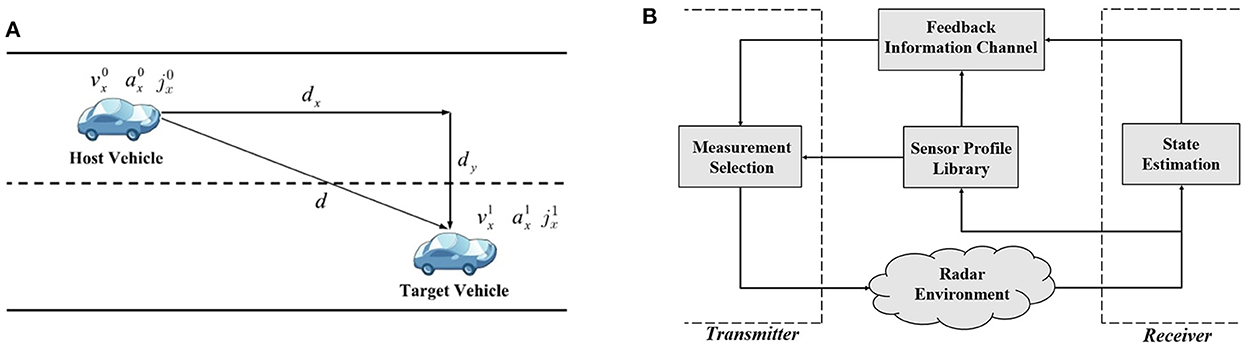
Figure 1. (A) A simple vehicle-following scenario (Feng and Haykin, 2018), and (B) the block diagram of the cognitive radar as an autonomous system (Zamiri-Jafarian and Plataniotis, 2022).

Reliable and accurate target tracking is the primary design goal of cognitive radar. To fulfill this objective, Figure 1B illustrates the general model of a cognitive radar as an example of S. Haykin's cognitive dynamic system (Haykin, 2012). In its most general structure, the cognitive radar includes a radar environment, a receiver, a feedback information channel, and a transmitter. According to Figure 1B, the target vehicle is embedded in the radar environment. The radar is equipped with a sensor profile library that contains distinct waveforms suitable for short and long-range applications. In a single cycle that takes place at one time instant, the system undergoes various stages. The receiver estimates the target's state (i.e., distance, velocity) by processing radar measurements and then conveys some form of this estimate to the transmitter through the feedback information channel. Based on the information provided by the receiver, the transmitter chooses the waveform—available from the sensor profile library—that contributes more to state estimation and leads to informative radar measurements. Lastly, the selected waveform is applied to the radar environment and the same cycle is repeated.

This paper proposes a comprehensive methodology to gain informative radar measurements that reduce the state estimation error on a cycle-by-cycle basis. In a recent article, the authors adopt a simple design where the sensor measures the impact of prospective waveforms—available from the sensor profile library—to state estimation and selects the one that maximizes the expectation of Bayesian surprise. Compared to the authors' work in Zamiri-Jafarian and Plataniotis (2022), this paper adopts a reinforcement learning technique with surprise-based intrinsic rewards to improve tracking performance mainly caused by risky driving situations (e.g., sudden stops). Figure 2 depicts the block diagram of a cognitive radar capable of learning from past transmissions and anticipating future responses by planning multiple time steps, which is inspired by Haykin's cognitive dynamic system (Haykin, 2012). To this end, the following introduces the model assumptions for designing the cognitive radar and mathematically formulates the objectives of this research.

FIGURE 2

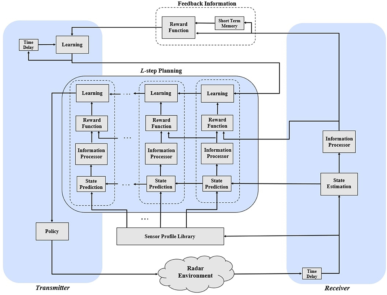
Figure 2. A learning design of cognitive radar for L-step planning.

2.1. Linear Gaussian dynamic system

For the simple driving scenario shown in Figure 1A, the paper assumes the radar measurements are constructed from a class of linear Gaussian state-space models (Simon, 2006), which at discrete time k are expressed as

$\begin{array}{l}{\text{x}}_{k+1}={\text{F}}_k{\text{x}}_k+{\text{w}}_k\\ {\text{z}}_k={\text{H}}_k{\text{x}}_k+{\text{v}}_k& (1)\end{array}$

where ${\text{x}}_k\in {ℝ}^n$, ${\text{F}}_k\in {ℝ}^{n\times n}$, and ${\text{w}}_k\in {ℝ}^n$ are respectively the state vector, the transition matrix, and the state noise; while ${\text{z}}_k\in {ℝ}^m$, ${\text{H}}_k\in {ℝ}^{m\times n}$, and ${\text{v}}_k\in {ℝ}^m$ denote the measurement vector, the measurement matrix, and the measurement noise, respectively. According to Equation 1, the evolution of the state follows first-order Markov-chain process and the noise elements are assumed additive zero-mean white Gaussian distribution (i.e., ${\text{w}}_k~{N}(0_{n\times 1},{\text{Q}}_k)$ and ${\text{v}}_k~{N}(0_{m\times 1},{\text{R}}_k)$). ${\text{Q}}_k\in {ℝ}^{n\times n}$ and ${\text{R}}_k\in {ℝ}^{m\times m}$ represent the state noise covariance and the measurement noise covariance, respectively. Furthermore, the initial state follows a Gaussian distribution, denoted as ${\text{x}}_0~{N}(\widehat{\text{x}}(0|0),\text{P}(0|0))$, and is mutually uncorrelated with the noise elements.

Depending on the driving scenario, the state x_k represents the entities of motion regarding the host and target vehicle, including distance, velocity, acceleration, etc. To emulate real-life highway and urban driving experiences, the following demonstrates two sets of linear Gaussian dynamic systems for constant acceleration and constant jerk.

2.1.1. Constant acceleration

For the case which constant acceleration is presumed during driving experience, x_k, is defined as follows

$\begin{array}{ll}{\text{x}}_k={\left[v_{x,k}^0,a_{x,k}^0,d_{x,k},v_{x,k}^1,a_{x,k}^1\right]}^T,& (2)\end{array}$

where $v_{x,k}^0$ and $a_{x,k}^0$ are the velocity and acceleration of the host vehicle; $v_{x,k}^1$ and $a_{x,k}^1$ are the velocity and acceleration of the target vehicle; d_x,k represents the longitude distance between the two vehicles. According to the equations of motion for constant acceleration, F_k and Q_k are derived as (Venhovens and Naab, 1999):

$\begin{array}{l}{\text{F}}_k=\left[\begin{array}{ccccc}1& T_s& 0& 0& 0\\ 0& 1& 0& 0& 0\\ -T_s& -T_s^2/2& 1& T_s& T_s^2/2\\ 0& 0& 0& 1& T_s\\ 0& 0& 0& 0& 1\end{array}\right],\\ {\text{Q}}_k=\left[\begin{array}{ccccc}{T}_s^4/4& T_s^3/2& -T_s^5/12& 0& 0\\ T_s^3/2& T_s^2& -T_s^4/6& 0& 0\\ -T_s^5/12& -T_s^4/6& T_s^6/18& T_s^5/12& T_s^4/6\\ 0& 0& T_s^5/12& T_s^4/4& T_s^3/2\\ 0& 0& T_s^4/6& T_s^3/2& T_s^2\end{array}\right]{\sigma }_q^2& (3)\end{array}$

where T_s and ${\sigma }_q^2$ refer to the sample time and the state noise variance, respectively. Assuming that the available radar measurements are the velocity of the target vehicle and the longitude distance, the measurement matrix becomes

$\begin{array}{ll}{\text{H}}_k=\left[\begin{array}{ccccc}0& 0& 0& 1& 0\\ 0& 0& 1& 0& 0\end{array}\right].& (4)\end{array}$

The measurement noise covariance depends on the waveform that the radar sensor transmits for target tracking. FMCW is the most standard modulation format, where linear frequency ramps with different slopes are conveyed (Roos et al., 2019). The FMCW modulation with Gaussian shaped pulse is commonly used in designing autonomous radars since it exhibits excellent range and velocity resolution. Hence, for a Gaussian shaped pulse with FMCW modulation, R_k is defined as follows (Kershaw and Evans, 1994):

$\begin{array}{l}{\text{R}}_k({\lambda }_{k-1},b_{k-1})=\\ \left[\begin{array}{cc}\frac{c^2}{{(2\pi f_c)}^2\eta }(\frac{1}{2{\lambda }_{k-1}^2}+2{\lambda }_{k-1}^2{b}_{k-1}^2)& -\frac{c^2{b}_{k-1}{\lambda }_{k-1}^2}{2\pi f_c\eta }\\ -\frac{c^2{b}_{k-1}{\lambda }_{k-1}^2}{2\pi f_c\eta }& \frac{c^2{\lambda }_{k-1}^2}{2\eta }\end{array}\right]& (5)\end{array}$

where λ_k−1, b_k−1, c, f_c, B and η are respectively the pulse duration, the chirp rate, the speed of light, the carrier frequency, signal bandwidth and the received signal-to-noise ratio (SNR). As shown in Equation 5, the measurement noise covariance depends on the pulse duration and chirp rate at k − 1 time index. This indicates the systems selection of the transmitted waveform (i.e., λ_k−1 and b_k−1) at the previous time cycle influences the radar measurements (i.e., z_k) at the current cycle. Note that both λ_k−1 and b_k−1 are the design parameters that signifies the radar waveform based on the tracking application (e.g., single or multiple target tracking). Since the transmitter and the receiver of the radar sensor are both mounted on the host vehicle, the received SNR for the target vehicle located at distance $d=\sqrt{d_x^2+d_y^2}$ maybe obtained as (Kershaw and Evans, 1994):

$\begin{array}{ll}\eta =(\frac{d_0}{d}{)}^4& (6)\end{array}$

where d_y is the lateral distance and d₀ is the distance at which 0 dB SNR is achieved.

2.1.2. Constant jerk

Implementing more practical driving scenarios (i.e., slowing down, detouring) requires an inconstant acceleration that varies over time. Since jerk is the acceleration derivative, we also determine the model parameters of Equation 1 for constant jerk. To do so, the state vector is defined as

$\begin{array}{ll}{\text{x}}_k={\left[\begin{array}{c}{v}_{x,k}^0,a_{x,k}^0,j_{x,k}^0,d_{x,k},v_{x,k}^1,a_{x,k}^1,j_{x,k}^1\end{array}\right]}^T& (7)\end{array}$

where $j_{x,k}^0$ and $j_{x,k}^1$ represent the jerk of the host vehicle and target vehicle, respectively. Consequently, F_k and Q_k are derived from the equations of motion with the assumption of constant jerk as follows

$\begin{array}{ll}{\text{F}}_k=\left[\begin{array}{ccccccc}1& T_s& T_s^2/2& 0& 0& 0& 0\\ 0& 1& T_s& 0& 0& 0& 0\\ 0& 0& 1& 0& 0& 0& 0\\ -T_s& -T_s^2/2& -T_s^3/6& 1& T_s& T_s^2/2& T_s^3/6\\ 0& 0& 0& 0& 1& T_s& T_s^2/2\\ 0& 0& 0& 0& 0& 1& T_s\\ 0& 0& 0& 0& 0& 0& 1\end{array}\right],& (8)\end{array}$

$\begin{array}{l}{\text{Q}}_k=\left[\begin{array}{ccccccc}{T}_s^6/36& T_s^5/12& T_s^4/6& -T_s^7/144& 0& 0& 0\\ T_s^5/12& T_s^4/4& T_s^3/2& -T_s^6/48& 0& 0& 0\\ T_s^4/6& T_s^3/2& T_s^2& -T_s^5/24& 0& 0& 0\\ -T_s^7/144& -T_s^6/48& -T_s^5/24& T_s^8/288& T_s^7/144& T_s^6/48& T_s^5/24\\ 0& 0& 0& T_s^7/144& T_s^6/36& T_s^5/12& T_s^4/6\\ 0& 0& 0& T_s^6/48& T_s^5/12& T_s^4/4& T_s^3/2\\ 0& 0& 0& T_s^5/24& T_s^4/6& T_s^3/2& T_s^2\end{array}\right]\\ {\sigma }_q^2.& (9)\end{array}$

Since the aim of the radar is to track $v_{x,k}^1$ and d_x,k, the measurement matrix is adjusted as follows

$\begin{array}{ll}{\text{H}}_k=\left[\begin{array}{ccccccc}0& 0& 0& 0& 1& 0& 0\\ 0& 0& 0& 1& 0& 0& 0\end{array}\right],& (10)\end{array}$

and the measurement noise covariance is computed from Equation 5.

While Equation 1 suffices to model the motion dynamics of simple driving situations, modeling complex driving scenarios that consider multiple targets requires switching dynamic models that may not necessarily be expressed as linear Gaussian dynamic systems.

2.2. Sensor profile library

As illustrated in Figure 2, the cognitive radar is equipped with a prescribed set of measurement noise covariances, referred to as the sensor profile library. It was discussed that the measurement noise covariance is computed based on the pulse duration and chirp rate (see Equation 5). The sensor profile library holds a large set of measurement noise covariances, denoted as ${R}$. Since going through the entire library at each time cycle to select the informative measurement (or optimum waveform) is computationally expensive and time-consuming, a localized set is considered instead. This paper adopts a k-Nearest Neighbours (kNN) method to obtain the localized set ${{R}}_k^{{L}}=\left\{{\text{R}}^{(1)},{\text{R}}^{(2)},...,{\text{R}}^{(N_{{L}})}\right\}\in {R}$, which includes measurement noise covariances that are neighbor to R_k. The work in Feng and Haykin (2018) views this localization approach as a form of an attention mechanism, which is one of the basic principles of cognition in modeling intelligent radar sensors.

2.3. Research objective

The ultimate goal of the cognitive radar is to estimate the target's state from the uncertain radar measurements while sustaining low estimation error on a cycle-by-cycle basis. Based on the model assumptions, this work aims to exploit how the sensor can manipulate the waveform signal parameters to improve the target's state estimate for the upcoming time cycle. To this end, the following presents the design objective in terms of a state estimation problem and proposes research questions on modeling the distinct blocks of cognitive radar.

Given the motion dynamics of the vehicle-following scenario is expressed by Equation 1; the state estimation problem becomes finding the estimated state, denoted as ${\widehat{\text{x}}}_k~p({\text{x}}_k|{\text{Z}}_k)$, that minimizes the following objective function at each time instant

$\begin{array}{ll}{\displaystyle \underset{{\widehat{\text{x}}}_k\in {ℝ}^n}{\text{arg min}}}𝔼\left[{\tilde{x}}_k^T{\tilde{x}}_k\right]& (11)\end{array}$

where ${\tilde{x}}_k={\text{x}}_k-{\widehat{\text{x}}}_k$ is the error between the true state and the estimated state, and p(x_k|Z_k) is the probability density function (PDF) of the estimated target's state given all radar measurements up to time k, denoted as Z_k. Equation 11 estimates the target's state and finds p(x_k|Z_k) that minimizes the mean squared error. This paper proposes the following research problems that address how a radar sensor can learn and plan to accomplish the design objective.

Research Problem 1. Suppose that the parameters of the model in Equation 1 are known. Determine the amount of new information in radar measurements that contribute to estimating the target's state ${\widehat{\text{x}}}_k$.

The first research problem captures the essence of the information processor in Figure 2. Computing the information of the estimated target's state is crucial because the sensor assigns reward values according to this information. Meanwhile, the following research problem deals with the nature of the reward and its connection to the design objective.

Research Problem 2. Let us consider that the action taken at the previous cycle is the transmitted waveform characterized by the measurement noise covariance, R_k. Assume a reward value is associated with the past action that indicates the consequence of previous waveform transmissions. Based on Research Problem 1, find a suitable function for the reward that drives the system to reduce the state estimation error.

The above problem models the feedback information channel in Figure 2, linking the information within the current state estimate provided by the receiver to the learning mechanism at the transmitter. Finally, the following provides the basis of the learning and planning algorithm in the context of reinforcement learning.

Research Problem 3. Let us consider that a set of measurement noise covariances ${{R}}_k^{{L}}$ are available (i.e., ${{R}}_k^{{L}}=\left\{{\text{R}}^{(1)},{\text{R}}^{(2)},\dots ,{\text{R}}^{(N_{{L}})}\right\}$). Derive the learning and planning algorithm for updating the value-to-go function and policy when multiple-step planning is applied.

3. Proposed approach

This section reviews the state-of-the-art including Haykin's design specific to cognitive radar (Haykin, 2012) and discusses an alternative approach that can apply to modeling such systems (Baldi, 2002). Lastly, our proposed solutions to Research Problems 1, 2, and 3 are presented.

3.1. Prior works

Numerous measures are suggested in statistics and information theory to quantify information (Shannon, 1948; Baldi, 2002; Friston, 2010). The most common is the Shannon entropy, which measures the amount of self-information or (Shannon surprise) of a particular observation, averaged over all possible outcomes (Shannon, 1948). In Haykin (2012) and Feng and Haykin (2018), the authors adopt the Shannon entropy to measure the information of the estimated target's state and model the information processor as follows:

$\begin{array}{l}{{H}}_k=-{\displaystyle {\int }_{{\text{x}}_k\in {ℝ}^n}}p({\text{x}}_k|{\text{Z}}_k)lnp({\text{x}}_k|{\text{Z}}_k)\text{d}{\text{x}}_k\\ =\frac{1}{2}ln\left[{(2\pi e)}^n\left|\text{P}(k|k)\right|\right]& (12)\end{array}$

where P(k|k) is the estimated state covariance when the Kalman filter is applied for state estimation (i.e., $p({\text{x}}_k|{\text{Z}}_k)={N}(\widehat{\text{x}}(k|k),\text{P}(k|k))$). Haykin further simplifies Equation 12 to ${{H}}_k=\left|\text{P}(k|k)\right|$ by making the case that the information within the target's state estimate is all captured in the determinant of the its covariance. To ensure that the system decreases the uncertainty in the state estimate between two subsequent cycles, Haykin defines the reward, denoted as r_k, in the following simple form (Fatemi and Haykin, 2014; Feng and Haykin, 2018):

$\begin{array}{ll}{r}_k=\frac{{\Delta }_k^{{H}}}{{{H}}_k}& (13)\end{array}$

where ${\Delta }_k^{{H}}={{H}}_{k-1}-{{H}}_k$ is the incremental deviation of the Shannon entropy at time k. The sign of ${\Delta }_k^{{H}}$ in Equation 13 guides the system to make the correct decision, where a positive reward indicates a reduction in estimation error due to the previous waveform transmission. At the same time, a negative one demonstrates a cost against the selected waveform.

While Haykin considers an information-theoretic approach, in a recent publication, the authors of this work proposed Bayesian surprise as the principal mechanism to acquire information (Zamiri-Jafarian and Plataniotis, 2022). The effect of the new radar measurement z_k on the target's state estimation is determined by measuring the Kullback–Leibler (KL) distance from the predicted PDF p(x_k|Z_k−1) to the posterior PDF p(x_k|Z_k) as follows:

$\begin{array}{l}{{S}}_k^B({\text{z}}_k)=D_{KL}(p({\text{x}}_k|{\text{Z}}_{k-1}),p({\text{x}}_k|{\text{Z}}_k))\\ ={\displaystyle {\int }_{{\text{x}}_k\in {ℝ}^n}}p({\text{x}}_k|{\text{Z}}_{k-1})ln\frac{p({\text{x}}_k|{\text{Z}}_{k-1})}{p({\text{x}}_k|{\text{Z}}_k)}\text{d}{\text{x}}_k& (14)\end{array}$

Appendix provides the closed-form expression for the Bayesian surprise when the Kalman filter is applied for state estimation. Although Haykin's approach is specific to cognitive radar, similar schemes can apply for deriving reward expressions given the choice of the information measure (e.g., Bayesian surprise).

3.2. Solution to research problem 1

In line with the authors' recent article, this paper proposes the Bayesian surprise as the main approach to quantify the amount of new information within the estimated state. In Zamiri-Jafarian and Plataniotis (2022), the authors investigate how the Bayesian surprise and its expectation provide valuable information to improve future state estimations given knowledge about prior estimates. With the assumption that the parameters of the linear Gaussian state-space models (see Equation 1) are somehow available, the Kalman filter is applied as the optimal estimator to obtain the state mean, $\widehat{\text{x}}(k|k)$, and its covariance matrix, P(k|k) (Simon, 2006). Algorithm 1 presents the two-step state prediction and estimation of the Kalman filter.

ALGORITHM 1

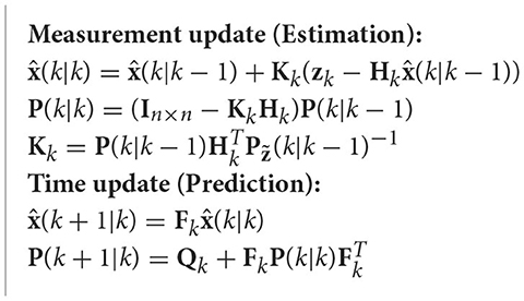
Algorithm 1. Kalman filter (Simon, 2006).

Since the research objective is reducing the mean squared error (see Equation 11), the expectation of the Bayesian surprise is more suitable to measure information rather than the Bayesian surprise. According to Equation A2 in Appendix, the expectation of Bayesian surprise with respect to $p({\text{z}}_k|{\text{Z}}_{k-1})~{N}({\text{H}}_k\widehat{\text{x}}(k|k-1),{\text{P}}_{\tilde{\text{z}}}(k|k-1))$ is computed as follows,

$\begin{array}{l}{𝔼}_{p({\text{z}}_k|{\text{Z}}_{k-1})}\left[{{S}}_k^B({\text{z}}_k)\right]=\\ \frac{1}{2}ln(|{\text{R}}_k{\text{P}}_{\tilde{\text{z}}}{(k|k-1)}^{-1}|)+\text{tr}\{{({\text{R}}_k{\text{P}}_{\tilde{\text{z}}}{(k|k-1)}^{-1})}^{-1}\}-m& (15)\end{array}$

where ${𝔼}_{p({\text{z}}_k|{\text{Z}}_{k-1})}[\left|\right|\tilde{\text{z}}(k|k-1)|{|}_{{\text{K}}_k^T\text{P}{(k|k)}^{-1}{\text{K}}_k}^2]$ is simplified to $\mathrm{\text{tr}}\{{({\text{R}}_k{\text{P}}_{\tilde{\text{z}}}{(k|k-1)}^{-1})}^{-1}\}-m$. According to Equation 15, the uncertainty in measurements balanced by what the filter perceives about the measurements (i.e., ${\text{R}}_k{\text{P}}_{\tilde{\text{z}}}{(k|k-1)}^{-1}$) influences the expectation of Bayesian surprise.

3.3. Solution to research problem 2

The second research problem deals with the nature of the reward and how it is defined for designing the feedback information channel in cognitive radar. In a classical reinforcement learning problem, the reward is a scalar value that measures the goodness of an action at a given state and is extrinsically predefined for all state-action pairs (Sutton and Barto, 2018). The algorithm aims to find suitable actions for a given situation to maximize some notion of reward. However, in cognitive radar, the reward is provided internally based on the sensor's belief about the radar measurements. To put it simply, let us assume that the transmitted waveform is the action the radar applies to the environment. The reward then reveals how good the previous transmission is according to the sensor's interpretation of the measurements, which is the information within the target's state estimate. The intrinsic nature of the reward in cognitive radar is undoubtedly an indication of autonomy.

As discussed, reward drives the radar to learn and make decisions that eventually lead to gaining informative measurements. Therefore, reward must be a function of the design objective, which is reducing the state estimation error on a cycle-by-cycle basis (see Equation 11). Since the paper considers the expectation of Bayesian surprise to measure the information within the target's state estimate, the author's propose the following basic requirements to express reward:

• Reward is a deterministic function that is proportional to the expectation of Bayesian surprise.

• Depending on the changes in the environment, the reward could assume a positive or negative value. A positive value is assigned when $𝔼[{{S}}_k^B]\le 𝔼[{{S}}_{k-1}^B]$ and a negative value is due to $𝔼[{{S}}_k^B]>𝔼[{{S}}_{k-1}^B]$.

The first condition is inspired by the work in Zamiri-Jafarian and Plataniotis (2022). Authors showed that, at a single instant, maximizing the expectation of Bayesian surprise leads to informative measurements. Therefore, it is reasonable that a measurement with a high expectation of Bayesian surprise is associated with a higher reward. Meanwhile, the rationality of the second requirement is traced back to the principle of free energy (Friston, 2010) which explains how adaptive systems (e.g., cognitive radar) resist a tendency to disorder. This principle suggests that autonomous systems learn and make better predictions by reducing the Bayesian surprise (or its expectation) from one cycle to the next. Here, we have assumed that the rule only applies to the previous cycle. To this end, the reward at time k is a function of the following two entities, given as

$\begin{array}{ll}{r}_k=g_k(𝔼\left[{{S}}_{k-1}^B\right],𝔼\left[{{S}}_k^B\right])& (16)\end{array}$

where g_k(.) is a deterministic function. There are different ways to define g_k(.) that align with the cognitive radar design objective. Note that finding the optimal function for reward is beyond this paper. To facilitate comparison with state-of-the-art methods, one choice is applying a similar approach to Haykin's reward, reintroduced as

$\begin{array}{ll}{r}_k=\frac{{\Delta }_k^{𝔼\left[{{S}}^B\right]}}{a+𝔼\left[{{S}}_k^B\right]}& (17)\end{array}$

where ${\Delta }_k^{𝔼[{{S}}^B]}=𝔼[{{S}}_{k-1}^B]-𝔼[{{S}}_k^B]$ is the incremental deviation of the expectation of Bayesian surprise computed at time k. In Equation 17, a is an arbitrary scaling value that is set by the algorithm (e.g., $a=𝔼[{{S}}_k^B]{|}_{k=0}$).

In addition to Equation 17, the paper presents alternative expressions for reward inspired by credibility measures in estimation and control theory (Li and Zhao, 2001, 2005, 2006). According to Li and Zhao (2001, 2005, 2006), the authors consider three metrics to determine the effectiveness of estimators in terms of reducing uncertainty in noisy measurements, which are: the Bayesian estimation error quotient (BEEQ), the estimate measurement error measure (EMER), and the Bayesian error reduction factor (BERF). Table 1 provides the mathematical definition of these three error measures. In Table 1, BEEQ quantifies the improvement of the mean estimate over its predicted version in the measurement-space, EMER evaluates the estimation process with respect to the measurements, and BERF computes the overall improvement of the estimation over both prediction and measurement update (Li and Zhao, 2006). The goal is to seek an expression based on these measures that particularly relate to the expectation of Bayesian surprise. The following shows the connection between Kalman filter covariance matrices and each metric in Table 1:

$\begin{array}{ll}\text{BEEQ}\propto {{O}}_M\left\{\frac{{\text{H}}_k\text{P}(k|k){\text{H}}_k^T}{{\text{H}}_k\text{P}(k|k-1){\text{H}}_k^T}\right\}={{O}}_M\left\{{\text{R}}_k{\text{P}}_{\tilde{\text{z}}}^{-1}(k|k-1)\right\},& (18)\end{array}$

$\begin{array}{l}\text{EMER}\propto \\ {{O}}_M\left\{\frac{{\text{H}}_k\text{P}(k|k){\text{H}}_k^T}{{\text{R}}_k}\right\}={{O}}_M\left\{{\text{I}}_{m\times m}-{\text{R}}_k{\text{P}}_{\tilde{\text{z}}}^{-1}(k|k-1)\right\},& (19)\end{array}$

where ${{O}}_M\{.\}$ represents a matrix operator such as the trace or the determinant. Meanwhile for BERF, the relation becomes

$\begin{array}{l}\text{BERF}\propto \\ \frac{{{O}}_M\left\{{\text{R}}_k{\text{P}}_{\tilde{\text{z}}}^{-1}(k|k-1)\right\}+{\beta }_k{{O}}_M\left\{{\text{I}}_{m\times m}-{\text{R}}_k{\text{P}}_{\tilde{\text{z}}}^{-1}(k|k-1)\right\}}{1+{\beta }_k}& (20)\end{array}$

where β_k is the error ratios of the predicted state mean to measurement, that is proportional to

$\begin{array}{l}{\beta }_k\propto {{O}}_M\left\{\frac{{\text{H}}_k\text{P}(k|k-1){\text{H}}_k^T}{{\text{R}}_k}\right\}=\\ {{O}}_M\{{({\text{R}}_k{\text{P}}_{\tilde{\text{z}}}^{-1}(k|k-1))}^{-1}-{\text{I}}_{m\times m}\}& (21)\end{array}$

Note that the expressions (Equations 18–20) depend on the term ${\text{R}}_k{\text{P}}_{\tilde{\text{z}}}{(k|k-1)}^{-1}$ that also appears in the expectation of Bayesian surprise. Thus, all of the above expression are suitable candidates to define the reward function. In this paper, we only concentrate on the BERF to express reward because β_k is closely related to the expectation of Bayesian surprise. Inspired by Equation 20, we propose the following reward expression

$\begin{array}{l}{r}_k=\frac{|{\text{R}}_{k-1}{\text{P}}_{\tilde{\text{z}}}^{-1}(k-1|k-2)|+\text{E}[{{S}}_{k-1}^B](|{\text{I}}_{m\times m}-{\text{R}}_{k-1}{\text{P}}_{\tilde{\text{z}}}^{-1}(k-1|k-2)|)}{1+\text{E}[{{S}}_{k-1}^B]}\\ -\frac{|{\text{R}}_k{\text{P}}_{\tilde{\text{z}}}^{-1}(k|k-1)|+\text{E}[{{S}}_k^B](|{\text{I}}_{m\times m}-{\text{R}}_k{\text{P}}_{\tilde{\text{z}}}^{-1}(k|k-1)|)}{1+\text{E}[{{S}}_k^B]}& (22)\end{array}$

where it satisfies both design requirements mentioned earlier. The possibility of using the trace or determinant for ${{O}}_M\{.\}$ is up to the designer. However, the determinant accounts for all valuable information in ${\text{R}}_k{\text{P}}_{\tilde{\text{z}}}^{-1}(k|k-1)$ (or ${\text{I}}_{m\times m}-{\text{R}}_k{\text{P}}_{\tilde{\text{z}}}^{-1}(k|k-1)$)—both diagonal and off-diagonal elements—rather than the trace. In Equation 22, $\text{E}[{{S}}_{k-1}^B]$ and ${\text{R}}_{k-1}{\text{P}}_{\tilde{\text{z}}}^{-1}(k-1|k-2)$ capture the change of the estimation error over subsequent cycles with respect to the BERF metric. A positive reward ensures that the preceding action works well in reducing the state estimation error. Furthermore, the computation of reward requires the knowledge of $𝔼[{{S}}_{k-1}^B]$ (see Equation 16). Since the feedback information channel in Figure 2 is responsible for determining the reward, a short-term memory block is presumed for designing the feedback information channel that accounts for the preceding expectation of Bayesian surprise. Though for complex reward functions (e.g., Equation 22), more memory is needed to design the feedback information channel.

TABLE 1

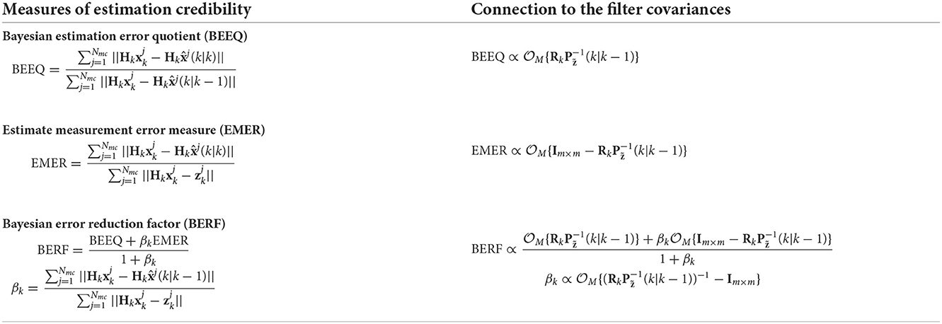
Table 1. A list of estimation credibility measures (Li and Zhao, 2001, 2005, 2006) and their connection to the filter's covariances.

3.4. Solution to research problem 3

The solution to the final research problem addresses the cognitive radar's learning and planning ability that implements the decision-making process. The policy and the value-to-go function are two main components (Sutton and Barto, 2018) in traditional reinforcement learning methods. The policy is the blueprint the decision-maker uses to select an action given knowledge of the current state of the environment. Meanwhile, the value-to-go function quantifies the performance of the policy by calculating the expected total reward for arbitrary action. The most popular dynamic programming approach in reinforcement learning is Q-learning, where the policy is the result of maximizing the value-to-go function. The following employs the same concepts to carry out the learning, planning, and policy stage of the cognitive radar depicted in Figure 2.

3.4.1. Learning

Learning is an important step that evaluates how much the system gains from the action taken in the previous cycle by computing the value-to-go function. As mentioned, the action refers to the measurement noise covariance that characterizes the radar signal waveform. Assuming that a set of measurement noise covariance is available from the sensor profile library (i.e., $\{{\text{R}}^{(1)},{\text{R}}^{(1)},...,{\text{R}}^{(N_{{L}})}\}$), the value-to-go function for a particular R is computed as follows

$\begin{array}{l}{V}_k(\text{R})={𝔼}^{\pi }\left[{\displaystyle \sum _{j=0}^{\infty }}{\gamma }^j{r}_{k+j}|{\text{R}}_k=\text{R}\right]\\ ={𝔼}^{\pi }\left[r_k+\gamma r_{k+1}+{\gamma }^2{r}_{k+2}+....|{\text{R}}_k=\text{R}\right]& (23)\end{array}$

where γ ∈ [0, 1) represents the discount factor that decreases the effect of future actions exponentially. Note that R_k = R is the measurement noise covariance selected at the previous time cycle, $\text{R}\in \{{\text{R}}^{(1)},{\text{R}}^{(1)},...,{\text{R}}^{(N_{{L}})}\}$. The expectation operator in Equation 23 is calculated with respect to the policy π. The policy π_k(R_k, R_k+1) is a probability distribution of the measurement noise covariance chosen at cycle k that includes the influence of the one at cycle k − 1. By applying the linear property of the expected value operator and the total probability theorem, Equation 23 can be simplified to

$\begin{array}{ll}{V}_k(\text{R})=r_k(\text{R})+\gamma {\displaystyle \sum _{j=1}^{N_{{L}}}}{\pi }_k(\text{R},{\text{R}}^{(j)})V_{k+1}({\text{R}}^{(j)})& (24)\end{array}$

where $r_k(\text{R})={𝔼}^{\pi }[r_k|{\text{R}}_k=\text{R}]$ is the reward function and the second term measures the effect of future selections. In addition, ${\pi }_k(\text{R},{\text{R}}^{(j)})$ is defined as follows

$\begin{array}{ll}{\pi }_k(\text{R},{\text{R}}^{(j)})=P\left\{{\text{R}}_{k+1}={\text{R}}^{(j)}|{\text{R}}_k=\text{R}\right\}& (25)\end{array}$

where P{.} computes the probability. To rewrite the value-to-go function in a recursive fashion, we have reformulated (Equation 24 by including a weighted incremental update of V_k(R), given as follows

$\begin{array}{l}{V}_k(\text{R})=V_{k-1}(\text{R})\\ +\alpha \left[r_k(\text{R})+\gamma {\displaystyle \sum _{j=1}^{N_{{L}}}}{\pi }_k(\text{R},{\text{R}}^{(j)})V_{k+1}({\text{R}}^{(j)})-V_{k-1}(\text{R})\right]& (26)\end{array}$

where α is the learning rate and V_k−1(R) is the value-to-go function of R from cycle k − 1. Given the reward r_k(R) and the value-to-go function V_k−1(R), Equation 26 computes how much the sensor learns from the immediate past transmission.

3.4.2. L-step planning

The planner is responsible for predicting the radar performance by considering the impact of future measurements through a series of hypothetical steps. The planner's function is to update the value-to-go function based on the predicted reward for a prescribed set of measurement noise covariances available from the sensor profile library. Compared to learning that occurs once in each cycle due to the preceding past action (i.e., R_k), the planning process takes place multiple times to go through a whole set of measurement noise covariances. Planning can extend to L stages, where each stage gives rise to a specific value-to-go function. The purpose of the L-step planning is to capture the influence of L future measurements in updating the value-to-go function so that the system can make a better decision.

Although planning executes the same tasks as learning, there is no interaction with the environment when planning is involved. Particularly, each measurement noise covariance available from the sensor profile library is virtually applied. For simplicity purposes, let us assume that there is only one-step planning (i.e., L = 1). As a result of virtually applying ${\text{R}}_{k+1}^{(i)}\in {{R}}_k^{{L}}$, the hypothesized state prediction Kalman algorithm for one-step planning becomes

$\begin{array}{ll}\text{P}(k+1|k)={\text{Q}}_k+{\text{F}}_k\text{P}(k|k){\text{F}}_k^T& (27)\end{array}$

$\begin{array}{ll}{\text{P}}_{\tilde{\text{z}}}^{(i)}(k+1|k)={\text{R}}_{k+1}^{(i)}+{\text{H}}_{k+1}\text{P}(k+1|k){\text{H}}_{k+1}^T& (28)\end{array}$

where P(k|k) is available due to the state estimation process, and ${\text{R}}_{k+1}^{(i)}$ is calculated from Equation 5 for $i=1,2,...,N_{{L}}$. The aim is to update the hypothesized value-to-go function, which requires the predicted reward associated to ${\text{R}}_{k+1}^{(i)}$. According to Equation 16, the expectation of Bayesian surprise is needed to compute the reward. Thus, the hypothesized expectation of Bayesian surprise with respect to p(z_k+1|Z_k) is given as

$\begin{array}{r}{𝔼}_{p({\text{z}}_{k+1}|{\text{Z}}_k)}[{{S}}_{k+1}^{B^{(i)}}]=\frac{1}{2}ln(|{\text{R}}_{k+1}^{(i)}{\text{P}}_{\tilde{\text{z}}}^{(i)}{(k+1|k)}^{-1}|)+\\ \text{tr}\{{({\text{R}}_{k+1}^{(i)}{\text{P}}_{\tilde{\text{z}}}^{(i)}{(k+1|k)}^{-1})}^{-1}\}-m& (29)\end{array}$

which leads to the following predicted value for the reward

$\begin{array}{ll}{r}_{k+1}^{(i)}({\text{R}}^{(i)})=g_{k+1}(𝔼[{{S}}_k^B],𝔼[{{S}}_{k+1}^{B^{(i)}}])& (30)\end{array}$

where $𝔼[{{S}}_k^B]$ was obtained earlier from Equation 15. g_k+1(.) can take any form of Equations 17 or 22. It is noteworthy to mention that the entities without the superscript (i) are the actual values and not the hypothesized ones. Finally, the value-to-go function as a result of the hypothesized action ${\text{R}}_{k+1}^{(i)}={\text{R}}^{(i)}$ is updated as

$\begin{array}{l}{V}_{k+1}^{(i)}({\text{R}}^{(i)})=V_k({\text{R}}^{(i)})\\ +\alpha \left[r_{k+1}^{(i)}({\text{R}}^{(i)})+\gamma {\displaystyle \sum _{i^{\prime }=1}^{N_{{L}}}}{\pi }_k({\text{R}}^{(i)},{\text{R}}^{(i^{\prime })})V_{k+2}({\text{R}}^{(i^{\prime })})-V_k({\text{R}}^{(i)})\right]& (31)\end{array}$

where we have omitted the time index in ${\text{R}}_{k+1}^{(i)}$ from the above equation to avoid confusion.

In addition for L-step planning, all the calculation through Equations (27–31) are carried out L number times, as shown in Figure 2. In this regard, the value-to-go function for L-step planning is obtained as

$\begin{array}{l}{V}_{k+L}^{(ij...rl)}({\text{R}}^{(l)})=V_{k+L-1}^{(ij...r)}({\text{R}}^{(l)})+\\ \alpha \left[r_{k+L}^{(ij...rl)}({\text{R}}^{(l)})+\gamma {\displaystyle \sum _{l^{\prime }=1}^{N_{{L}}}}{\pi }_k({\text{R}}^{(l)},{\text{R}}^{(l^{\prime })})V_{k+L+1}^{(ij...r)}({\text{R}}^{(i^{\prime })})-V_{k+L-1}^{(ij...r)}({\text{R}}^{(l)})\right]& (32)\end{array}$

where (ij...l) represents the sequence of L future measurement noise covariances selected from the sensor profile library, denoted as (R⁽ⁱ⁾, R^(j), ..., R^(l)), such that ${\text{R}}^{(i)}\in {{R}}_k^{{L}},{\text{R}}^{(j)}\in {{R}}_{k+1}^{{L}},...,{\text{R}}^{(l)}\in {{R}}_{k+L-1}^{{L}}$ and $i,j,...,l=\{1,...,N_{{L}}\}$. Meanwhile, $r_{k+L}^{ij...rl}({\text{R}}^{(l)})=g_{k+L}(𝔼[{{S}}_{k+L-1}^{B^{(ij...r)}}],𝔼[{{S}}_{k+L}^{B^{(ij...rl)}}])$ corresponds to the reward as a result of the mentioned configuration.

3.4.3. Policy

Updating the policy is the final procedure in designing the cognitive radar. Policy is the rule used by the sensor to decide what to do given the knowledge about the current state of the environment. In fact, the purpose of both learning and planning is to improve the policy and guide the sensor toward informative measurements. For that matter, a mixed strategy that balances between exploitation and exploration is desirable in updating the policy. Hence, this article uses the ϵ-greedy strategy to select the measurement noise covariance for the next time cycle. With the input of the policy block being ${\{V_{k+L}^{(ij...rl)}\}}_{i=1}^{N_{{L}}}$, R_k+1 based on the ϵ-greedy strategy is chosen as

$\begin{array}{ll}{\text{R}}_{k+1}=\{\begin{array}{cc}{\text{R}}^{(i)}\in {{R}}_k^{{L}}& \text{with probability }ϵ\\ \\ {\displaystyle \underset{{\text{R}}^{(i)}\in {{R}}_k^{{L}}}{\text{argmax}}}{V}_{k+L}^{(ij...rl)}& \text{with probability }1-ϵ\end{array}& (33)\end{array}$

where with probability ϵ (e.g., 0.05) the radar selects R_k+1 randomly (exploration) and with probability 1 − ϵ (e.g., 0.95) the maximum value-to-go function is chosen (exploitation). The result in Equation 33 is the action that is applied to the radar environment. To this end, the policy is updated according to the following expression

$\begin{array}{ll}{\pi }_{k+1}({\text{R}}_k,{\text{R}}_{k+1})=\{\begin{array}{l}P\left\{{\text{R}}_{k+1}\in {{R}}_k^{{L}}|{\text{R}}_k\right\}=\frac{ϵ}{N_{{L}}}\\ \\ P\{{\text{R}}_{k+1}={\displaystyle \underset{{\text{R}}^{(i)}\in {{R}}_k^{{L}}}{\text{argmax}}}{V}_{k+L}^{(ij...rl)}|{\text{R}}_k\}=1-ϵ+\frac{ϵ}{N_{{L}}}\end{array}& (34)\end{array}$

which is then used to compute the value-to-go function for learning and planning at the next cycle.

Algorithm 2 illustrates the proposed cognitive radar algorithm for learning and L-step planning, where the expectation of Bayesian surprise drives the sensor to acquire informative radar measurements. Note that a similar process, with some minor modifications, applies to modeling the cognitive radar based on other definitions of surprise when learning and L-step planning is considered. Table 2 lists the various forms of measuring the information within the target's state estimate and its corresponding reward function. As previously mentioned, Haykin approximates the Shannon entropy (defined in Equation 12 as ${{H}}_k=\left|\text{P}(k|k)\right|$. While he argues that all the information about the target's state is captured by the determinant of the estimated state covariance, this approximation may lead to different results. In this regard, Table 2 presents two alternative forms of Haykin's approach to numerically investigate the impact of this approximation.

ALGORITHM 2

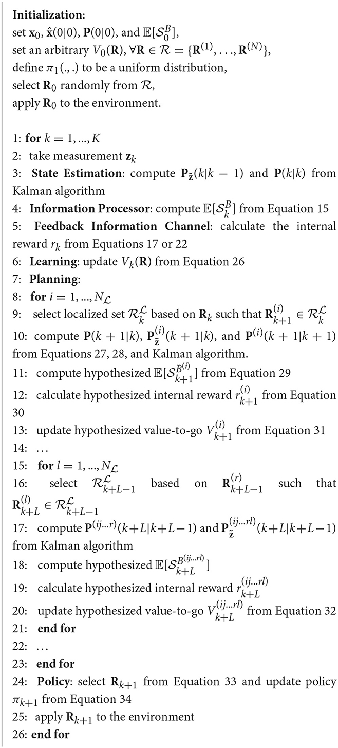
Algorithm 2. Cognitive radar based on learning and L-step planning.

TABLE 2

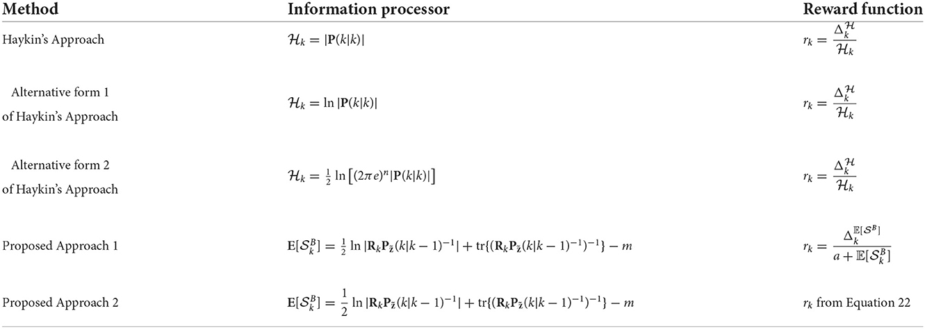
Table 2. Various methods of modeling the cognitive radar.

4. Simulation results

In this section, simulation results are presented to compare the state estimation performance of the proposed cognitive radar with state-of-the-art (Fatemi and Haykin, 2014; Feng and Haykin, 2018). The following demonstrates the simulation setup and parameter settings for generating radar measurements that emulate the vehicle-following scenario in Figure 1A. Similar to our recent work (Zamiri-Jafarian and Plataniotis, 2022), we suggest a radar configuration suitable for single-target tracking in practical environments. Two driving experiences are implemented to examine various aspects of the estimation performance. This section compares the system performance of the proposed learning and planning algorithm to its alternative competitor for different reward functions. The impact of multiple-step planning in improving state estimation performance is also analyzed through a series of experiments. Results are verified over numerous Monte Carlo runs.

4.1. Simulation setup and data generation

The intention of this experiment is to evaluate the estimation performance of the proposed cognitive radar. Since the paper adopts the Kalman filter to perform state estimation, the model parameters in Equation 1 (i.e., F_k, Q_k, H_k, R_k, $\widehat{\text{x}}(0|0)$ and P(0|0)) are assumed given. In this regard, the sensor layout and the parameter setting for generating radar measurements are presented.

For the vehicle-following scenario shown in Figure 1A, the simulation assumes that the two cars are moving forward in the same lane (i.e., d_y = 0). In this simulation, the FMCW radar sensor is positioned on the host vehicle and operates in the 77 GHz frequency band for short- and long-range applications (Hasch et al., 2012). The bandwidth of the transmitted radar signal is set to B = 100 MHz, and 0 dB SNR is achieved at d₀ = 2000 m. According to Equation 5, the measurement noise covariance is a function of pulse duration and the chirp rate, R_k(λ_k−1, b_k−1). By assuming that the radar sensor maintains a maximum range of d_max = 100 m and a maximum velocity of v_max = 100 m/s, the sensor profile library consists of measurement noise covariances specified for the following values:

$\begin{array}{l}{\lambda }_{k-1}\in \left[10e-7:e-7:10e-6\right]\cup \left[1.1e-6:e-6:10e-5\right],\\ b_{k-1}\in \left[-e12:0.2e12:-0.2e12\right]\cup \left[0.2e12:0.2e12:e12\right],\end{array}$

where λ_k−1 and b_k−1 are configured to simulate a practical radar sensor for single-target tracking applications (Roos et al., 2019). The sensor profile library is composed of N = 1, 810 measurement noise covariances, denoted as ${R}={\{{\text{R}}^{(i)}({\lambda }_{k-1},b_{k-1})\}}_{i=1}^N$. Since N is a large number, and searching the entire library at each cycle is cost-ineffective, this paper adopts the kNN method to obtain a smaller set with $N_{{L}}=25$ members. Figure 3 illustrates an example of a localized set of measurement noise covariance, ${{R}}_k^{{L}}$, that is specified by pulse duration and chirp rate.

FIGURE 3

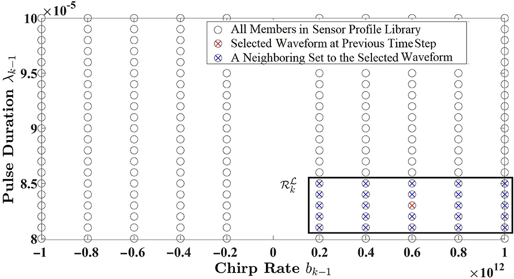
Figure 3. An example of a neighboring set ${{R}}_k^{{L}}$ with $N_{{L}}=25$ members (Zamiri-Jafarian and Plataniotis, 2022).

This article demonstrates two driving experiences to evaluate the state estimation performance of the proposed cognitive radar: (i) a simple highway driving scenario and (ii) adjusting to a sudden stop in an urban environment. For the highway driving experience, we consider the dynamics of two cars are expressed as Equations (3–5) when constant acceleration is presumed. Since the true initial state, x₀, and its estimation elements (i.e., $\widehat{\text{x}}(0|0)$, P(0|0)) depend on the driving environment, without loss of generality, the true initial state for highway driving is set to

$\begin{array}{l}{\text{x}}_0={\left[25\text{ m/s},3{\text{ m/s}}^2,100\text{ m},23\text{ m/s},2{\text{ m/s}}^2\right]}^T,\end{array}$

while the initial estimation of the state mean and its covariance matrix are assumed as

$\begin{array}{l}\widehat{\text{x}}(0|0)={\left[24\text{ m/s},3{\text{ m/s}}^2,80\text{ m},23\text{ m/s},2{\text{ m/s}}^2\right]}^T,\end{array}$

$\begin{array}{l}\text{P}(0|0)=\text{diag}(\left[100,1,100,100,1\right]).\end{array}$

A practical in-city driving encounter includes slowing down and stopping due to unpredictable circumstances (e.g., rash driving, careless pedestrians, and severe weather conditions). To examine how the proposed cognitive radar learns and adapts in such risky situations, we present the following driving scenario. Let us assume that initially the target vehicle is driving with constant velocity. At the sight of an unexpected event, the target vehicle suddenly hits the brakes and comes to a stop. The host vehicle that is following the target vehicle with constant velocity—to avoid an accident—also hits the breaks and slows down, until it comes to a complete stop behind the target vehicle with a safe distance. Given that hitting the breaks changes the acceleration linearly, we consider the model parameters of constant jerk introduced in Equations (8–10). To this end, x₀, $\widehat{\text{x}}(0|0)$, and P(0|0) are set to

$\begin{array}{l}{\text{x}}_0\\ ={\left[16.7\text{ m/s},0{\text{ m/s}}^2,0{\text{ m/s}}^3,27.8\text{ m},13.9\text{ m/s},0{\text{ m/s}}^2,0{\text{ m/s}}^3\right]}^T,\\ \widehat{\text{x}}(0|0)={\left[16\text{ m/s},0{\text{ m/s}}^2,0{\text{ m/s}}^3,27\text{ m},13\text{ m/s},0{\text{ m/s}}^2,0{\text{ m/s}}^3\right]}^T,\\ \text{P}(0|0)=\text{diag}(\left[100,1,1,100,100,1,1\right]),\end{array}$

where the values are adjusted according to an urban environment. Figure 4 illustrates how the actual state vector entities—velocity, acceleration, jerk, and the longitude distance— change over time based on the suggested driving scenario. Note that the estimated initial state ${\widehat{\text{x}}}_0~{N}(\widehat{\text{x}}(0|0),\text{P}(0|0))$ is a random value that changes per Monte Carlo run. This simulation sets the state noise variance to ${\sigma }_q^2=0.01$ and the sample time T_s = 0.1 s for computing F_k and Q_k to ensure constant acceleration in highway driving and constant jerk in urban driving. Finally, the learning rate, the discount factor, and the greedy factor in this simulation are assigned as α = 0.1, γ = 0.5 and ϵ = 0.1, respectively.

FIGURE 4

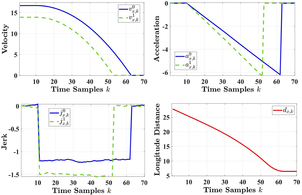
Figure 4. The true state vector dynamics for the urban driving experience.

4.2. Metrics and performance evaluation

This paper considers the root mean square error (RMSE) to evaluate the estimation performance of the proposed cognitive radar, defined as

$\begin{array}{ll}{\text{RMSE}}_k=\sqrt{\frac{1}{N_{mc}}{\displaystyle \sum _{j=1}^{N_{mc}}}\Vert {\text{x}}_k^j-{\widehat{\text{x}}}^j(k|k){\Vert }^2}& (35)\end{array}$

where ${\text{x}}_k^j$ and ${\widehat{\text{x}}}^j(k|k)$ are the state vector and the estimated state vector of the j-th Monte Carlo simulation at time step k, respectively. N_mc represents the number of Monte Carlo simulations. For performance comparison, the paper adopts the various schemes listed in Table 2.

4.2.1. Learning with one-step planning

This section presents the estimation response of the proposed radar design by tracking the velocity of the target vehicle, $v_{x,k}^1$, and the longitude distance, d_x,k, when learning with one-step planning are involved. The experiment examines target tracking in highway and urban driving scenarios. Results are obtained for N_mc = 10,000 Monte Carlo runs.

Figures 5A,B, respectively, illustrate the RMSE performance of longitude distance and velocity of the target vehicle for the highway driving experience. The results are plotted in a logarithm scale for the duration of 10 s. Let us first compare Haykin's design with its alternative approaches. As shown in both figures, the alternative forms of Haykin's design outperform his approach, indicating that the approximation of Equation 12 leads to different results. This inconsistency implies that the estimation performance is numerically sensitive to the choice of the information processor in computing the reward value. Despite some instances, alternative form 2—which is the full Shannon entropy expression—presents a lower error level than its approximation forms. In the meantime, our proposed techniques based on the expectation of Bayesian surprise significantly exceed Haykin's design. Although proposed approach 1 has a similar reward function to Haykin's scheme, the expectation of Bayesian surprise provides sufficient information to improve the state estimation process compared to the determinant of the estimated state covariance. Note that in this simulation, we have set $a=𝔼[{{S}}_k^B]{|}_{k=0}$ to normalize the reward function with respect to the initial expected Bayesian surprise. Since the order of $𝔼[{{S}}_k^B]$ drastically varies (i.e., toward a minimum), we have included a to obtain a smooth and normalized reward. While the latter experiences a higher error level than alternative forms 1 and 2, our second proposed approach significantly surpasses all the other designs by a landslide. This is due to the fact that the suggested reward expression based on the BERF credibility measure aligns with successively reducing the state estimation error.

FIGURE 5

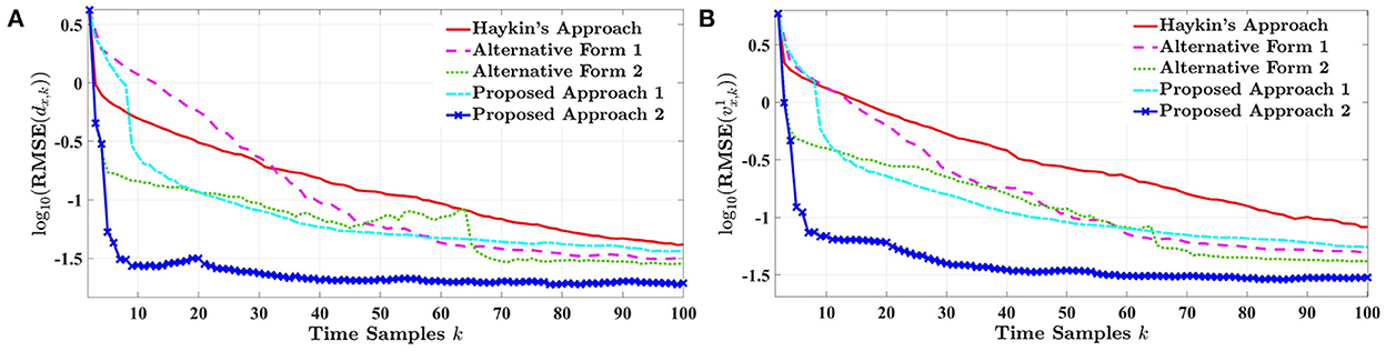
Figure 5. The RMSE of (A) the longitude distance and (B) the target's velocity for one-step planning in highway driving.

Figures 6A,B, depict the RMSE curves of the longitude distance and target velocity when the vehicle-following scenario takes place in an urban environment, respectively. As previously discussed, this experiment evaluates the tracking performance of the cognitive radar for the methods listed in Table 2 when the target vehicle unexpectedly brakes and stops. Results are simulated for 7 s. Since the dynamics of the true state vector changes according to Figure 4, the estimation performance of the longitude distance and target velocity drastically shifts in two time instances, when (i) the acceleration of the target vehicle starts to decrease (i.e., braking), and (ii) the target vehicle comes to a complete stop. As shown in both figures, our proposed radar design based on approach 2 can adapt to these sudden changes and experiences a minimum level of estimation error compared to the state-of-the-art. This confirms that the proposed reward expression in Equation 22 inspired by the BERF credibility measure provides sufficient information to enhance system performance for unforeseen driving situations. On the other hand, Haykin's design presents the poorest RMSE response in tracking d_x,k and $v_{x,k}^1$. Similar to highway driving, the estimation responses of Haykin's approach and its alternative forms are hypersensitive to the reward value for different approximations of the Shannon entropy. However, in this experiment, the first alternative form of Haykin's approach is ranked second among the other methods. Results show that the log determinant of the estimated state covariance significantly outperforms its subgroup competitors in tracking the state dynamics.

FIGURE 6

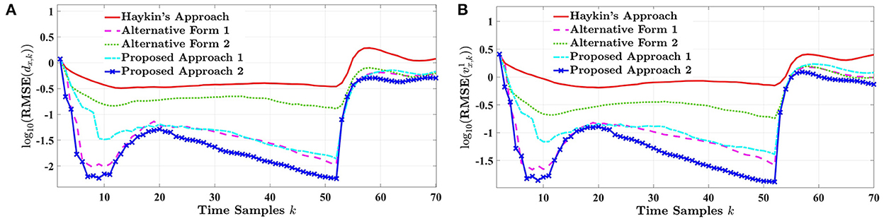
Figure 6. The RMSE of (A) the longitude distance and (B) the target's velocity for one-step planning in urban driving.

4.2.2. Learning with L-step planning

This section evaluates the estimation performance of the proposed cognitive radar when the impact of L future measurements is considered in estimating the target's state for the upcoming time cycle. The results of this experiment are averaged over N_mc = 5, 000 Monte Carlo simulations for both highway and urban driving scenarios. Since the RMSE results are more distinguishable for $v_{x,k}^1$, the following only focuses on how the estimation of the target's velocity improves when multiple-step planning is assumed. Meanwhile, the same conclusion for estimating the target's velocity also applies to the longitude distance. Note that we have included the curves that challenge our proposed approach 2 and Haykin's approach.

Figure 7A illustrates the RMSE performance of the cognitive radar for L = {1, 2} in highway driving. In the case of highway driving, the estimation response of Haykin's approach, alternative form 2, and our proposed approach 2 are plotted for one-step and two-step planning. As shown, the estimation error substantially decreases by increasing the planning step from one to two. However, for our proposed radar design, the error reduction by changing L = 1 to L = 2 does not improve compared to Haykin's method and alternative form 2. While all three ways eventually merge for two-step planning, our second approach provides a smoother estimation response over time. Furthermore, this section investigates the impact of multiple-step planning for tracking the target velocity in risky driving situations. For the unexpected stopping scenario in an urban environment, Figure 7B depicts the RMSE performance of Haykin's approach, alternative form 1, and our proposed approach 2 when L = 1 and L = 2. Although Haykin's approach improves considerably by an additional planning step, its alternative form 1 in some time instances experiences a higher estimation error for two-step planning in contrast to one. In the meantime, the estimation performance of our proposed approach 2 fails for planning two time-steps, especially right after the target vehicle hit's the brake and slows down (i.e., k ∈ [11, 53]). The results from alternative form 1 and the paper's approach imply that increasing the planning step in unpredictable driving circumstances does not necessarily lead to better tracking performance. Even though Haykin's design presents a lower error for L = 2 (i.e., compared to L = 1), our proposed cognitive radar for L = 1 outperforms all other techniques regardless of the time-step planning. This is particularly observed when the cognitive radar tries to adapt to the sudden stop by the target vehicle, after time sample k = 10 in Figure 7B. Since increasing L is associated with a longer simulation run time and higher computational complexity, on average, our model for one-step planning displays an adequate state estimation response. Therefore, it seems that for driving scenarios where the dynamics of the environment change abruptly, multiple-step planning is not an optimum solution.

FIGURE 7

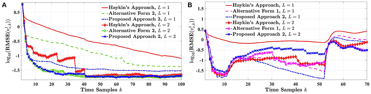
Figure 7. The RMSE of the target's velocity for L = {1, 2} and N_mc = 5, 000 in (A) highway driving and (B) urban driving.

5. Conclusion

This article proposed a surprise-based learning and planning algorithm for the cognitive radar that internally computes rewards based on the expectation of Bayesian surprise and decides on future waveform transmissions by minimizing the estimation error over time. The radar measurements were constructed from two sets of linear Gaussian state-space models that describe the motion dynamics of a simple vehicle-following scenario for constant acceleration and constant jerk. Assuming that the model parameters are given, this paper applied the Kalman filter for state estimation and the expectation of Bayesian surprise to measure the information within the filter's estimate. The sensor assigned intrinsic reward values depending on the expectation of Bayesian surprise to signify the goodness of the preceding action and updated the value-to-go function accordingly. Through a series of hypothetical planning steps, the radar evaluated the contribution of each prospective waveform—available from the sensor profile library—to estimate the target's future state (i.e., velocity, distance), and it chose the one based on an exploitation-exploration strategy. Several experiments were carried out to examine and compare the estimation performance of the proposed method to the state-of-the-art. Numerical results were implemented to emulate real-life highway and urban driving experiences. Results demonstrated that the reward expressions inspired by credibility measures in control and estimation theory are more suitable for achieving informative radar measurements. Specifically, this research focused on the Bayesian error reduction factor (BERF) for defining rewards since it considered both the prediction process and the measurement update, which captures the exact essence of the Bayesian surprise. For one-step planning, the proposed cognitive radar exceeds its competitor's estimation performance with respect to the mean squared error (RMSE). The paper also showed that our approach for one-step planning displays lower errors in risky driving situations than the alternative designs for two-step planning.

Data availability statement

The original contributions presented in the study are included in the article/supplementary material, further inquiries can be directed to the corresponding author.

Author contributions

KP and YZ-J contributed to the study's conceptualization, methodology, and statistical analysis. YZ-J investigated, validated, implemented the results of the paper, and wrote the first draft of the manuscript. KP supervised and administered the work and with MH provided the funding for this research. All authors contributed to the manuscript revision, read, and approved the submitted version.

Funding

This project was partially supported by the Department of National Defence's Innovation for Defence Excellence and Security (IDEaS) program, Canada.

Conflict of interest

The authors declare that the research was conducted in the absence of any commercial or financial relationships that could be construed as a potential conflict of interest.

Publisher's note

All claims expressed in this article are solely those of the authors and do not necessarily represent those of their affiliated organizations, or those of the publisher, the editors and the reviewers. Any product that may be evaluated in this article, or claim that may be made by its manufacturer, is not guaranteed or endorsed by the publisher.

References

Baldassarre, G., and Mirolli, M. (2013). Intrinsically Motivated Learning in Natural and Artificial Systems. Berlin: Springer.

Google Scholar

Baldi, P. (2002). “A computational theory of surprise,” in Information, Coding and Mathematics (Boston, MA: Springer), 1–25.

Google Scholar

Baldi, P., and Itti, L. (2010). Of bits and wows: a bayesian theory of surprise with applications to attention. Neural Netw. 23, 649–666. doi: 10.1016/j.neunet.2009.12.007

PubMed Abstract | CrossRef Full Text | Google Scholar

Barto, A., Mirolli, M., and Baldassarre, G. (2013). Novelty or surprise? Front. Psychol. 11, 907. doi: 10.3389/fpsyg.2013.00907

PubMed Abstract | CrossRef Full Text | Google Scholar

Bell, K. L., Baker, C. J., Smith, G. E., Johnson, J. T., and Rangaswamy, M. (2015). Cognitive radar framework for target detection and tracking. IEEE J. Sel. Top. Signal Process. 9, 1427–1439. doi: 10.1109/JSTSP.2015.2465304

CrossRef Full Text | Google Scholar

Çatal, O., Leroux, S., De Boom, C., Verbelen, T., and Dhoedt, B. (2020). “Anomaly detection for autonomous guided vehicles using bayesian surprise,” in 2020 IEEE/RSJ International Conference on Intelligent Robots and Systems (IROS) (Las Vegas, NV: IEEE), 8148–8153.

Google Scholar

Faraji, M., Preuschoff, K., and Gerstner, W. (2018). Balancing new against old information: the role of puzzlement surprise in learning. Neural Comput. 30, 34–83. doi: 10.1162/neco_a_01025

PubMed Abstract | CrossRef Full Text | Google Scholar

Fatemi, M., and Haykin, S. (2014). Cognitive control: theory and application. IEEE Access 2, 698–710. doi: 10.1109/ACCESS.2014.2332333

CrossRef Full Text | Google Scholar

Feng, S., and Haykin, S. (2018). Cognitive risk control for transmit-waveform selection in vehicular radar systems. IEEE Trans. Vehicular Technol. 67, 9542–9556. doi: 10.1109/TVT.2018.2857718

CrossRef Full Text | Google Scholar

Friston, K. (2010). The free-energy principle: a unified brain theory? Nat. Rev. Neurosci. 11, 127. doi: 10.1038/nrn2787

PubMed Abstract | CrossRef Full Text | Google Scholar

Greco, M. S., Gini, F., Stinco, P., and Bell, K. (2018). Cognitive radars: on the road to reality: progress thus far and possibilities for the future. IEEE Signal Process. Mag. 35, 112–125. doi: 10.1109/MSP.2018.2822847

CrossRef Full Text | Google Scholar

Gurbuz, S. Z., Griffiths, H. D., Charlish, A., Rangaswamy, M., Greco, M. S., and Bell, K. (2019). An overview of cognitive radar: Past, present, and future. IEEE Aerospace Electron. Syst. Mag. 34, 6–18. doi: 10.1109/MAES.2019.2953762

CrossRef Full Text | Google Scholar

Hakobyan, G., and Yang, B. (2019). High-performance automotive radar: a review of signal processing algorithms and modulation schemes. IEEE Signal Process. Mag. 36, 32–44. doi: 10.1109/MSP.2019.2911722

CrossRef Full Text | Google Scholar

Hasch, J., Topak, E., Schnabel, R., Zwick, T., Weigel, R., and Waldschmidt, C. (2012). Millimeter-wave technology for automotive radar sensors in the 77 ghz frequency band. IEEE Trans. Microw. Theory Tech. 60, 845–860. doi: 10.1109/TMTT.2011.2178427

CrossRef Full Text | Google Scholar

Haykin, S. (2006). Cognitive radar: a way of the future. IEEE Signal Process. Mag. 23, 30–40. doi: 10.1109/MSP.2006.1593335

CrossRef Full Text | Google Scholar

Haykin, S. (2012). Cognitive Dynamic Systems: Perception-Action Cycle, Radar and Radio. Cambridge: Cambridge University Press.

Google Scholar

Haykin, S., Xue, Y., and Setoodeh, P. (2012). Cognitive radar: Step toward bridging the gap between neuroscience and engineering. Proc. IEEE 100, 3102–3130. doi: 10.1109/JPROC.2012.2203089

CrossRef Full Text | Google Scholar

Hou, M., Banbury, S., and Burns, C. (2014). Intelligent Adaptive Systems: An Interaction-Centered Design Perspective. Boca Raton, FL: CRC Press.

Google Scholar

Hou, M., Ho, G., and Dunwoody, D. (2021). Impacts: a trust model for human-autonomy teaming. Hum. Intell. Syst. Integr. 3, 79–97. doi: 10.1007/s42454-020-00023-x

CrossRef Full Text | Google Scholar

Hou, M., Wang, Y., Trajkovic, L., Plataniotis, K. N., Kwong, S., Zhou, M., et al. (2022). Frontiers of brain-inspired autonomous systems: how does defense r&d drive the innovations? IEEE Syst. Man Cybern. Mag. 8, 8–20. doi: 10.1109/MSMC.2021.3136983

CrossRef Full Text | Google Scholar

Hussain, R., and Zeadally, S. (2018). Autonomous cars: research results, issues, and future challenges. IEEE Commun. Surveys Tutorials 21, 1275–1313. doi: 10.1109/COMST.2018.2869360

PubMed Abstract | CrossRef Full Text | Google Scholar

Itti, L., and Baldi, P. (2009). Bayesian surprise attracts human attention. Vis. Res. 49, 1295–1306. doi: 10.1016/j.visres.2008.09.007

PubMed Abstract | CrossRef Full Text | Google Scholar

Jo, K., Kim, J., Kim, D., Jang, C., and Sunwoo, M. (2015). Development of autonomous car–part ii: a case study on the implementation of an autonomous driving system based on distributed architecture. IEEE Trans. Ind. Electron. 62, 5119–5132. doi: 10.1109/TIE.2015.2410258

CrossRef Full Text | Google Scholar

Kershaw, D. J., and Evans, R. J. (1994). Optimal waveform selection for tracking systems. IEEE Trans. Inf. Theory 40, 1536–1550. doi: 10.1109/18.333866

CrossRef Full Text | Google Scholar

Li, X. R., and Zhao, Z. (2005). “Relative error measures for evaluation of estimation algorithms,” in 2005 7th International Conference on Information Fusion, Vol. 1 (Philadelphia, PA: IEEE), p. 8.

Google Scholar

Li, X. R., and Zhao, Z. (2006). “Measuring estimator's credibility: noncredibility index,” in 2006 9th International Conference on Information Fusion (Florence: IEEE), 1–8.

Google Scholar

Li, X. R., and Zhao, Z. (2001). “Measures of performance for evaluation of estimators and filters,” in Signal and Data Processing of Small Targets 2001, Vol. 4473 (San Diego, CA: SPIE), 530–541.

Google Scholar

Liakoni, V., Modirshanechi, A., Gerstner, W., and Brea, J. (2021). Learning in volatile environments with the bayes factor surprise. Neural Comput. 33, 269–340. doi: 10.1162/neco_a01352

PubMed Abstract | CrossRef Full Text | Google Scholar

Neel, A. (2018). Lidar vs. Radar. Available online at: https://www.fierceelectronics.com/components/lidar-vs-radar

Palm, G. (2012). Novelty, Information and Surprise. Berlin: Springer Science & Business Media.

Google Scholar

Proff, H., Bowman, K., Tanaka, Y., Zhou, A., Kim, T. H., Singh, R., et al. (2022). 2021 Global Automotive Consumer Study: Global Focus Countries. Available online at: https://www2.deloitte.com/content/dam/Deloitte/us/Documents/manufacturing/us-2021-global-automotive-consumer-study-global-focus-countries.pdf

Roos, F., Bechter, J., Knill, C., Schweizer, B., and Waldschmidt, C. (2019). Radar sensors for autonomous driving: modulation schemes and interference mitigation. IEEE Microwave Mag. 20, 58–72. doi: 10.1109/MMM.2019.2922120

CrossRef Full Text | Google Scholar

Shannon, C. E. (1948). A mathematical theory of communication. Bell Syst. Techn. J. 27, 379–423. doi: 10.1002/j.1538-7305.1948.tb01338.x

PubMed Abstract | CrossRef Full Text | Google Scholar

Simon, D. (2006). Optimal State Estimation: Kalman, H Infinity, and Nonlinear Approaches. Hoboken, NJ: John Wiley & Sons.

Google Scholar

Sokcevic, M. (2022). Safe and Fun-Modern Cars Must Have it All. Available online at: https://www.tttech-auto.com/expert_insight/modern-cars-must-have-it-all

Stahl, A. E., and Feigenson, L. (2015). Observing the unexpected enhances infants learning and exploration. Science 348, 91–94. doi: 10.1126/science.aaa3799

PubMed Abstract | CrossRef Full Text | Google Scholar

Sutton, R. S., and Barto, A. G. (2018). Reinforcement Learning: An Introduction. Cambridge, MA: MIT Press.

Google Scholar

Venhovens, P. J. T., and Naab, K. (1999). Vehicle dynamics estimation using kalman filters. Vehicle Syst. Dyn. 32, 171–184. doi: 10.1076/vesd.32.2.171.2088

CrossRef Full Text | Google Scholar

Wang, Y., Karray, F., Kwong, S., Plataniotis, K. N., Leung, H., Hou, M., et al. (2021a). On the philosophical, cognitive and mathematical foundations of symbiotic autonomous systems. Philos. Trans. R. Soc. A 379, 20200362. doi: 10.1098/rsta.2020.0362

PubMed Abstract | CrossRef Full Text | Google Scholar

Wang, Y., Pitas, I., Plataniotis, K. N., Regazzoni, C. S., Sadler, B. M., Roy-Chowdhury, A., et al. (2021b). “On future development of autonomous systems: a report of the plenary panel at IEEE ICAS 21,” in 2021 IEEE International Conference on Autonomous Systems (ICAS) (Montreal, QC: IEEE), 1–9.

Google Scholar

Zamiri-Jafarian, Y., and Plataniotis, K. N. (2020). “Bayesian surprise in linear gaussian dynamic systems: revisiting state estimation,” in 2020 IEEE International Conference on Systems, Man, and Cybernetics (SMC) (Toronto, ON: IEEE), 3387–3394.

Google Scholar

Zamiri-Jafarian, Y., and Plataniotis, K. N. (2022). A bayesian surprise approach in designing cognitive radar for autonomous driving. Entropy 24, 672. doi: 10.3390/e24050672

PubMed Abstract | CrossRef Full Text | Google Scholar

Appendix

Closed-form expressions for the Bayesian surprise are possible in both state-space and measurement-space (Zamiri-Jafarian and Plataniotis, 2022). Given that $p({\text{x}}_k|{\text{Z}}_{k-1})={N}(\widehat{\text{x}}(k|k-1),\text{P}(k|k-1))$ and $p({\text{x}}_k|{\text{Z}}_k)={N}(\widehat{\text{x}}(k|k),\text{P}(k|k))$ are available from the Kalman filter in Algorithm 1, the Bayesian surprise from Equation 14 is simplified to

$\begin{array}{l}{{S}}_k^B({\text{z}}_k)=\frac{1}{2}[ln\frac{|\text{P}(k|k)|}{|\text{P}(k|k-1)|}+\text{tr}\left\{\text{P}{(k|k)}^{-1}\text{P}(k|k-1)\right\}\\ -n+\Vert \widehat{\text{x}}(k|k)-\widehat{\text{x}}(k|k-1){\Vert }_{\text{P}{(k|k)}^{-1}}^2]& (\mathrm{A1})\end{array}$

where $\widehat{\text{x}}(k|k)$, $\widehat{\text{x}}(k|k-1)$, P(k|k − 1), and n are the estimated state mean, the predicted state mean, the predicted state covariance matrix, and the state-space dimension, respectively. Meanwhile, the Bayesian surprise in the measurement-space is derived as

$\begin{array}{r}{{S}}_k^B({\text{z}}_k)=\frac{1}{2}[ln|{\text{R}}_k{\text{P}}_{\tilde{\text{z}}}{(k|k-1)}^{-1}|-m+\\ \Vert \tilde{\text{z}}(k|k-1){\Vert }_{{\text{K}}_k^T\text{P}{(k|k)}^{-1}{\text{K}}_k}^2+\text{tr}\{{({\text{R}}_k{\text{P}}_{\tilde{\text{z}}}{(k|k-1)}^{-1})}^{-1}]& (\mathrm{A2})\end{array}$

where $\tilde{\text{z}}(k|k-1)={\text{z}}_k-{\text{H}}_k\widehat{\text{x}}(k|k-1)$ is the innovation vector, ${\text{P}}_{\tilde{\text{z}}}(k|k-1)={\text{R}}_k+{\text{H}}_k\text{P}(k|k-1){\text{H}}_k^T$ is the innovation covariance, and m is the dimension of the measurement space. Due to the nature of the problem in this paper, we focus on the Bayesian surprise expression in measurement-space.