Bio-Inspired Multimodal Imaging in Reduced Visibility

The visual systems found in nature rely on capturing light under different modalities, in terms of spectral sensitivities and polarization sensitivities. Numerous imaging techniques are inspired by this variety, among which, the most famous is color imaging inspired by the trichromacy theory of the human visual system. We investigate the spectral and polarimetric properties of biological imaging systems that will lead to the best performance on scene imaging through haze, i.e., dehazing. We design a benchmark experiment based on modalities inspired by several visual systems, and adapt state-of-the-art image reconstruction algorithms to those modalities. We show the difference in performance of each studied systems and discuss it in front of our methodology and the statistical relevance of our data.

1 Introduction

A wide variety of visual systems can be found in nature. Those systems sense light with different spectral sensitivities and polarization sensitivities. Presumably, those visual systems are optimally adapted for specific conditions, e.g., some animals develop specific sensitivities to permit navigation or prey detection (Horváth et al., 2014). It is also known that some animals can potentially use spectral or polarization information to increase the visibility through turbid media (Horváth et al., 2014). Airlight can reduce the visibility in a natural environment. It comes when the atmospheric particles, e.g., water droplets, ice crystals, dust, or smoke, are lit directly or indirectly by the Sun. Light scattering causes a modification of the signal according to the radiative transfer theory, that in imaging causes a decrease in contrast with distance and a loss of color fidelity (El Khoury et al., 2014; El Khoury et al., 2018a).

The radiance of the scene captured by a camera sensor can be written like in Eq. 1,

$I=\int f(\lambda )s(\lambda )d\lambda ,(1)$

where f(λ) is the radiance, and s(λ) is the spectral sensitivity of the sensor. The radiance of the scene is the combination of the contributions from the objects in the scene and from the airlight present in a scene observed through a turbid media. The radiance from the scene is proportional to the irradiance of the sensor for a given aperture and a given focal length. In our work, when we mention radiance, it is the contribution of the radiance of the scene to the imaging process. The total radiance results from a contribution by the object in the scene, J, and by the airlight, A, as defined by the Koschmieder (Koschmeider, 1924) solution to the radiative transfer equation, as in Equation (2), where α and γ are the contributions to each of the components with γ = 1 − α:

$I=\alpha J+\gamma A,(2)$

Thus we can rewrite Eq. 1 as Eq. 3, where j(λ) is the contribution of the object in the scene by wavelengths λ, and a(λ) is the airlight spectral characteristics.

$I=\int (\alpha j(\lambda )+(1-\alpha )a(\lambda ))s(\lambda )d\lambda .(3)$

To inverse the Koschmieder model, the parameters to retrieve are the radiance due to the airlight a(λ), and the transmittance α that defines how the light is traversing the air. This also gives the attenuation (1 − α) of the atmosphere largely due to scattering, and more moderately through absorption. Without atmospheric particles, the transmittance α = e^−βd is close to 1, where β (in m⁻¹) is the extinction coefficient invariant with the distance d. The computer vision community proposes several methods to estimate those parameters (Ancuti et al., 2019) amongst which one class is based on image statistics in intensity (He et al., 2011), and another on the difference of intensity between polarization modes (Schechner et al., 2003). In those two cases, it is assumed that the density of haze is uniform in the scene. Today’s literature proposes to inverse this problem using machine learning techniques, e.g. AoD-net (Li et al., 2017), Dehazenet (Cai et al., 2016), or conditional GAN (Li et al., 2018).

In this communication, we investigate 1) whether the extra information modalities sensed by various animals could potentially help them in hazy/reduced-visibility conditions and more generally in some turbid media, and 2) if so, whether we could improve state-of-the-art image information recovery by designing imaging systems for computer vision applications. To this end, we design a benchmark experiment for performance evaluation of several bio-inspired spectral and polarimetric visual systems on image dehazing. As the experiment is designed considering only the spectral range and polarization sensitivity of the animal’s visual systems, the cognitive process of the animals in performing dehazing is not considered in this work. We rather freely design and test bio-sensors of equivalent spatial resolutions. The imaging systems could be physically implemented with current state-of-the-art techniques: general filter arrays, filter wheels, line-scan, or multiple camera set-ups.

The experimental data is captured in a hazy environment, with a multispectral and polarization imaging system. We merge those data and reconstruct the normalised radiance for the different polarization angles, which allow us to emulate any animal sensory system for which the physiology is known. We then use and adapt state-of-the-art hazy image reconstruction algorithms to the spectro-polarimetric modalities. Results could help the design or co-design of sensors for computer vision, while perhaps also give some indications on how animal visual systems may be used to navigate in turbid media such as fog.

We first describe the acquisition setup and the pre-processing steps to generate the data in Section 2. Then, we simulate the bio-inspired sensor images from the data, dehaze and visualize them in Section 3. Finally, results and analysis are provided in Section 4, before concluding in Section 5.

2 Data Acquisition and Construction

This section describes the acquisition and the pre-processing of spectral and polarimetric images. The existing haze datasets like O-haze (Ancuti et al., 2018a), I-haze (Ancuti et al., 2018b), NH-Haze (Ancuti et al., 2020), CHIC (El Khoury et al., 2018b), or Dense Haze (Ancuti et al., 2019) are all color image based. There exists one dataset that is spectral, SHIA (El Khoury et al., 2020), but does not cover polarization neither UV. It is therefore not possible to obtain spectral or polarization data out of these. We decided to capture the data ourselves from the available cameras. We also define a pipeline (see Figure 1) that transforms the raw captured data into a standard data representation of high dynamic range spectral images, with 5 nm resolution in the UV-A and visible domain, and four states of polarization.

FIGURE 1

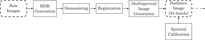
FIGURE 1. Data acquisition pipeline. Raw images are captured using a CPFA camera with four polarization angles, in front of spectral bandpass filters as described in Section 2.1. Pre-processing steps (HDR, demosaicing, and registration) are described in Section 2.1, whereas spectral image reconstruction is described in Section 2.2. The dotted arrow corresponds to the connection toward Figure 3.

2.1 Data Capture

We combine three cameras for the capture. Two of them are Color Polarization Filter Array (CPFA) cameras with the IMX250 MYR sensor by SONY. Each of these two cameras is combined with a spectral filter attached to the lens: the first one with a blue-green BG39 filter, and the second with the yellow GG475 filter (both manufactured by Schott), so that at the end, we obtain six visible bands. The other one is a Polarization Filter Array (PFA) camera with the IMX250 MZR sensor by SONY. To capture the UV-A range of the spectrum, it is combined with a bandpass UG1 filter (manufactured by Schott) and a BG39 filter to avoid the red transmission of the UG1 filter. Finally, the complete camera system has a total of 28 channels: seven spectral channels with four polarization channels each. The sensitivities of the cameras are in Figure 2A, and the transmittance of the spectral filters are in Figure 2B. The total spectral sensitivity of the system is in Figure 2C.

FIGURE 2

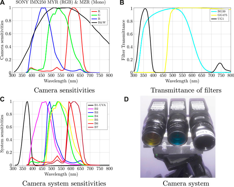
FIGURE 2. (A) Normalized spectral sensitivities of the two cameras used. (B) Transmittance of the bandpass filters. (C) Total system sensitivity, which is a combination of the camera sensitivities with the bandpass filters. We show only spectral sensitivities for the 0° polarization channels as spectral sensitivities of all polarization channels are very similar.

We capture the outdoor scene simultaneously and with three different exposure times. We apply the fusion HDR process proposed by Debevec and Malik (Paul, 1997) directly on raw images and by pixel (Lapray et al., 2017). It avoids under or over saturated values and balances energy and noise among all spectro-polarimetric channels. Then, to recover the full spatial resolution, we applied the state-of-the-art demosaicing technique dedicated to PFA/CPFA images (Morimatsu et al., 2020). Finally, we register all the bands using the speeded up robust features (SURF) method (Bay et al., 2006) to compensate for any misalignment induced by field of view or optical assembly.

2.2 Spectral Reconstruction

With this seven band multispectral system, we want to be able to simulate any physiological sensory system. We separate the UV band from the rest and estimate the visible range radiant information as a function of λ from the sensor integrated values. We apply a well-established method that uses the pseudo-inverse method (Maloney and Wandell, 1986) to convert camera signals to spectral reflectance factors. We choose the Xrite Macbeth ColorChecker (MCC) as a calibration target, with 24 patches with known reflectance properties. The reflectance of the patches are used to train the model. We set a resolution of 5nm between 380 and 780nm, resulting in M = 81 equally-spaced wavelengths. Assuming that the camera system has a linear response, we compute the matrix W as follows:

$\mathbf{W}={\mathbf{F}}_{\mathbf{train}}{\mathbf{I}}_{\mathbf{train}}^{+},(4)$

where the + superscript symbol is the pseudoinverse operation of a non-square matrix (we used the pinv function in Matlab, i.e. the Moore-Penrose method), W is a 81 × 6 matrix, I_train is a matrix of size 6 × 24 formed by column vectors containing the captured camera signals of the 24 patches of the calibration target, and F_train is a 81 × 24 matrix representing the spectral reflectance of patches.

Once the transformation matrix W is known, we can estimate the spectral data p (81 × 1) from camera signals (taken with the same lightning conditions) at each pixel position by:

$\mathbf{p}=\mathbf{W}\mathbf{I},(5)$

where I is a 6 × 1 vector containing the camera signals. To evaluate the calibration precision, we apply Equation 5 to other captured signals of another reference target (the creative reference chart of the Xrite ColorChecker Passport, the one presented in Figure 4C of (Lapray et al., 2018)). The calibration results and the RMSE errors between the estimated and reference spectra are very similar to those presented in Figure 7 of (Lapray et al., 2018).

From any scene captured by our camera system, we then have spectral scene data that can be used to simulate any spectral sensing.

3 Experiment

In this section, we first describe how we transform the spectral data generated from the previous section into bio-inspired sensor data. In a second time, we explain the extension of the dehazing algorithms to multimodal images and the visualisation procedure as color images. The process is summarized in Figure 3.

FIGURE 3

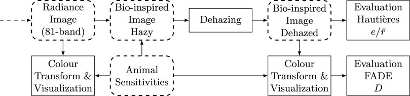
FIGURE 3. Design of the second step of processing. From the radiance image, we simulate the sensing process, apply dehazing and evaluate the result according to image data. An alternative color visualization pipeline permits looking at colour images and provide an alternative evaluation of the result. The dotted arrow corresponds to the connection from Figure 1.

3.1 Animal Sensitivities

The set of selected animal visual systems are summarized in Table 1: 1) Dogs or pigs are dichromates, 2) primates are trichromates (equivalent to the human color vision system); 3) Papilio butterflies have polarization sensitivities for each of the three spectral bands, 4) Cricket have three spectral bands and two polarization orientations in the short wavelengths; 5) Zebra-fish has four spectral bands spanning UV and color; 6) Avian has five spectral channels.

TABLE 1

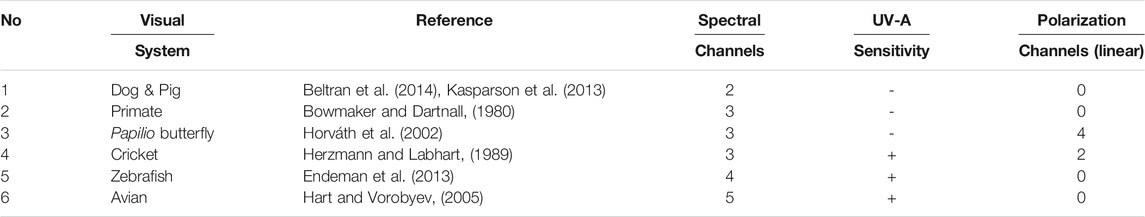
TABLE 1. Summary of the visual systems. We used sensitivities presented in the literature from physiological studies of animal visual systems. Three of the animals are sensitive to the UV, and two are sensitive to polarization.

The spectral sensitivities S of each animal are shown in Figure 4. We aim at investigating if the visibility is enhanced with an increasing number of channels and modalities, and potentially identify trends that may give a better result.

FIGURE 4

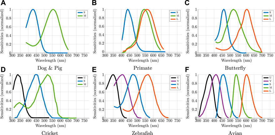
FIGURE 4. Normalized spectral sensitivities S of each selected animals. U, V, S, M, and L refer to the ultraviolet (UV-A), violet (VS), short-wavelength (SWS), medium-wavelength (MWS), and long-wavelength-sensitive (LWS) cones respectively. The names only indicate the approximate peak wavelength and are different between the animals.

For the polarization blind animals (dog/pig, primate, zebrafish, and avian), we use the dehazing method based on the airlight estimation from dark-channel prior (He et al., 2011), as described later in Section 3.4.1, which extension to an arbitrary number of bands is trivial.

Insects like crickets use UV-A for navigation so that they can identify the position of the Sun, even in difficult environments or cloudy days, relatively to the patches of the sky that are visible. The cricket has a UV-A sensitive channel that combines a polarization sensitivity in the dorsal rim area. This behavior is partly explained in (Barta and Horváth, 2004) and (Von Frisch, 2013), where it is said that although the degree of polarization is generally lower in the UV than in the visible (called ”UV-sky-pol paradox”) in clear skies, the polarization of light is highest in UV when reflected from clouds/canopies, and is the least sensitive to “atmospheric disturbances.” Although this part of its visual system probably does not generate a very resolved image, we assume that the cricket can use a discrete airlight estimation based on few partial observations. The highest spatial resolution is only for the other spectral sensitivities in the rest of the photoreceptors. For the cricket, we apply the polarization-based method (Schechner et al., 2003), as described later in Section 3.4.2, taking the same airlight estimation (in the UV-A channel) to dehaze all the spectral bands.

Other insects use polarization sensitivity for prey or food detection, like transparent prey where the polarization signature difference with the background is more pronounced than the spectral one. The butterfly has jointly the linear polarization (with four different angles of analysis) and colors sensitivities to detect flowers from the background environment (Horváth et al., 2014). Contrary to the cricket, the polarization sensitivity is for all spectral channels. For this animal, we can apply the polarization-based method (Schechner et al., 2003) initially proposed by the authors without modification.

3.2 Simulation of Bio-Inspired Sensing

Each bio-inspired system is composed of N sensors (N = 2 for dogs, N = 3 for primates, etc.), as shown in Figure 4. The N sensors are represented as M-dimensional column vectors s_i i( indexes the channel number), gathered in a M × N matrix S.

The simulation of sensor values I′ (N × 1) pertaining to a specific visual system shown in Figure 4, are computed using spectral data p from Eq. 5 as:

$\begin{array}{c}\hfill {\mathbf{I}}^{\prime }={\mathbf{G}\mathbf{S}}^{\mathbf{t}}\mathbf{p},\end{array}(6)$

where $\mathbf{G}=\mathrm{diag}\left(\frac{1}{\max {({\mathbf{S}}^{\mathbf{t}}\mathbf{p})}_i}\right)$ is a normalization matrix on sensor values, where i goes over all the N spectral sensors.

All simulated data are spatially gathered to form an image and applied on each visual system in Figure 4. All the simulated data will be used later in Section 3.4 as an input for the dehazing algorithms.

The simulated spectral data will be provided online when the paper is published. The link will be included in the final version.

3.3 Data Visualization as Color Images

In order to visualize the data from the sensors, we propose to convert them into color images. This is achieved by defining an orthogonal basis of the sensor space, and projecting the data from this space to a colorspace.

Given the previously generated spectra p with M channels, we can find a projection of p to the subspace spanned by the N sensors. To this end, we make an orthonormal basis of the sensor subspace, by applying a Gram–Schmidt QR decomposition to S:

$\begin{array}{c}\hfill \mathbf{S}=\mathbf{Q}\mathbf{R}=\left[\begin{array}{cc}\hfill {\mathbf{Q}}_{\mathbf{1}}\hfill & \hfill {\mathbf{Q}}_{\mathbf{2}}\hfill \end{array}\right]\left[\begin{array}{c}\hfill {\mathbf{R}}_{\mathbf{1}}\hfill \\ \hfill 0\hfill \end{array}\right],\end{array}(7)$

where Q is an M × M orthogonal matrix, Q₁ an M × N matrix with orthonormal columns spanning the same space as the columns of S, Q₂ an M × (M − N) matrix with orthonormal columns spanning the null space of S, R an M × N upper triangular matrix, and R₁ an N × N upper triangular matrix. To project the individual pixel spectrum p onto the sensor subspace, and reconstruct a pixel spectrum represented as a column vector p′, we use:

$\begin{array}{c}\hfill {\mathbf{p}}^{\prime }={\mathbf{Q}}_{\mathbf{1}}{({\mathbf{R}}_{\mathbf{1}}^{\mathbf{t}})}^{-\mathbf{1}}{\mathbf{G}}^{-\mathbf{1}}{\mathbf{I}}^{\prime },\end{array}(8)$

note that I′ could come from either a hazy or dehazed sensor intensity value.

Then, we can compute the corresponding CIEXYZ values from each animal’s p′ for illustrative purpose:

$\begin{array}{c}\hfill \left[\begin{array}{c}\hfill X\hfill \\ \hfill Y\hfill \\ \hfill Z\hfill \end{array}\right]={\mathbf{C}}^{\mathbf{t}}{\mathbf{p}}^{\prime },\end{array}(9)$

where C (M × 3) are the CIE (1931) Color Matching Functions (CMFs) (Wright, 1929; Guild and Petavel, 1931). Then, we convert the CIEXYZ values to sRGB (Standard (1999)) for visualization. The results, both for hazy and dehazed data, are shown in Figure 5.

FIGURE 5

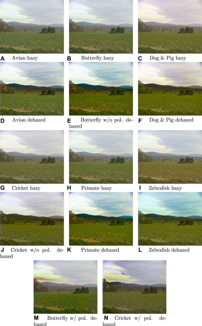
FIGURE 5. sRGB visualization (scene 1) of images before and after dehazing for each animal.

3.4 Adaptation of Dehazing Algorithms for Each Sensor

We adapt two algorithms from the state-of-the-art: the Dark Channel Prior (DCP) method from (He et al., 2011); and a polarization-based image reconstruction (Schechner et al., 2003).

3.4.1 Extension of DCP to Spectral Images

DCP was previously applied to spectral images (Martínez-Domingo et al., 2020). Our adaptation is based on the code provided by Matlab (imreducehaze function, “approxdcp” option), which is the direct implementation of the algorithm by He et al. (He et al., 2011). First, an extension of the Dark Channel Prior is done for spectral data. Initially, the algorithm computes the dark channel by taking the minimum over the RGB values of a small local patches of 15 × 15 pixels. The assumption of dehazing using dark channel is based on a statistical observation which demonstrates that the fog-free images have a dark channel image with very low pixel intensities. We can assume that we have the same statistical behavior for N ≠ 3, so that we can extend the dark channel computation over all the available spectral channels. Nevertheless, this assumption should be verified over a large dataset of hazy and fog-free multispectral images when available.

Moreover, the DCP method uses guided filtering (He et al., 2013) to refine the transmission map. Initially, the guidance image was in RGB, so that all the three channels are used for guidance (color statistics) for filtering the transmission map. The guided filtering has not been generalized to the spectral case yet. The average spectral channel should correspond quite well to a luminance/greyscale image, so we decided to use an average image over all spectral channels as a guidance image.

3.4.2 Adaptation of Schechner Method in Bio-Inspired Sensors

The algorithm of Schechner et al. (2003) estimates the airlight map by assuming that the light scattered by atmospheric particles is partially polarized. They compute the degree of linear polarization and assume that the induced polarization is only due to scattering. The separation of the radiance of the object and the airlight is done per spectral band, relatively to the amount of polarization detected in the spectral channel.

For the butterfly case, we compute the airlight map independently and by channel, as the polarization sensitivity is available for the three bands. The dehazing is done per spectral channel using the corresponding airlight map.

For the cricket, we compute the airlight only in the UV-A channel (as cricket has only the polarization sensitivity in the UV-A channel), and apply the algorithm to dehaze all spectral channels using this unique airlight estimation.

4 Data Analysis

4.1 Metrics

The evaluation of results is done on images both in the sRGB color space and by spectral channel. It is not possible in our case to use the metrics with reference (e.g. PSNR, SSIM, CIEDE 2000) because the ground truth does not exist. Thus, we have selected some metrics that are without references or with the fog image as reference.

The first metric used is FADE (D) by Choi and You (2015). This metric is applied on color images, and is based on Natural Scene Statistics (NSS) and fog aware statistical features. D is computed on a single image and gives a low value for a low fog perception.

The second metric used is by Hautière et al. (2011). It measures the improvement in the visibility of objects present in a scene before and after processing, using contrast descriptors. Two parameters are given by the metric: e and $\bar{r}$. The rate of new visible edges is depicted as e, whereas the restoration quality (geometric mean ratios of visible gradients) is $\bar{r}$. The parameter $\bar{r}$ takes into account both visible and non-visible edges. Two input images (foggy and dehazed) are needed to assess the restoration quality. Higher $e/\bar{r}$ values mean better performance in contrast restoration.

4.2 Results

We captured two case study scenes. One scene is a more rural area (taken at Mortzwiller, France), and can be described as an open landscape, though some houses can be seen. The second scene is a more urban context (taken at Mulhouse, France), with nevertheless some trees. The degree of fog varies between the two scenes.

The scores computed by the metrics are shown in Tables 2, 3.

TABLE 2

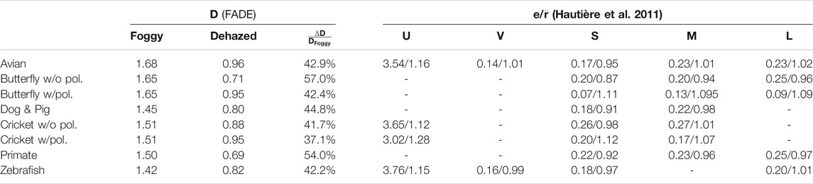
TABLE 2. Evaluation results of dehazing for scene 1. The evaluation metric D (FADE (Choi and You, 2015)) is applied on sRGB images, whereas the metrics e and $\bar{r}$ (Hautière et al., 2011) are applied per spectral channel.

TABLE 3

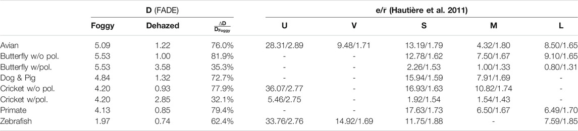
TABLE 3. Evaluation results of dehazing for scene 2. The evaluation metric D (FADE (Choi and You, 2015)) is applied on sRGB images, whereas the metrics e and $\bar{r}$ (Hautière et al., 2011) are applied per spectral channel.

4.2.1 FADE

The hazy and dehazed sRGB images on which FADE was computed are shown in Figures 5, 6.

FIGURE 6

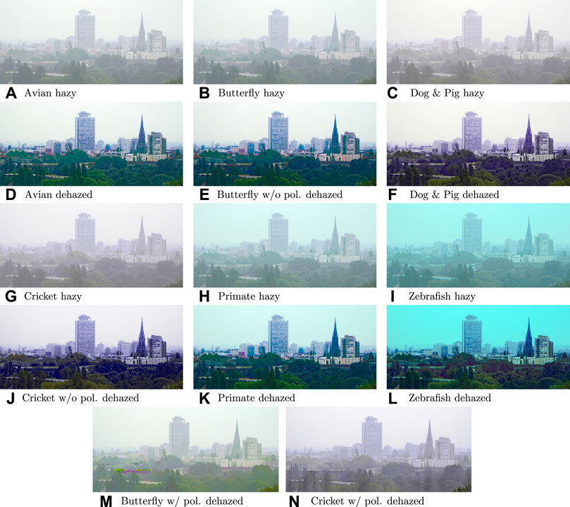
FIGURE 6. sRGB visualization (scene 2) of images before and after dehazing for each animal.

The FADE metric provides different results for the color version of the foggy images captured by different sensors. FADE varies from 1.42 to 1.68 for scene 1, and from 1.97 to 5.53 for scene 2. The difference of range and scores of the FADE metric is easily related to the difference in the quantity of fog present in the scenes. The best FADE metric is always to the images captured by the Zebrafish inspired sensor, while the worst images according to the metric are the Butterfly and the avian.

All FADE scores improved after dehazing. Improvement for scene 1 ranges from 47.1% for the Cricket to 57% for the Butterfly. The polarized versions did not improve as much as the unpolarized versions. For scene 2, improvement is larger and ranges from 32.1% for the Cricket without polarization to 81.9% for the Butterfly. For the dehazed images, the Butterfly without polarization and the Zebrafish, provide the best FADE scores for scene 1 and 2 respectively. The animals that give the best relative improvement of the D metric after dehazing are the Butterfly (without polarization) and the primate.

We remark that increasing the number of spectral bands for the reconstruction of a color image does not necessarily give better results for the FADE metric. For example, the case of the dog gives better results than that of the avian or cricket.

For the polarization based-method, we can see that the perception of haze is globally reduced between hazy and dehazed images, but to a smaller degree than that without polarization. It can be explained by the fact that the polarization method reduces the presence of fog less than the DCP method. The estimation of the airlight using polarization for each band (butterfly) instead of just one band (cricket) does not appear to provide a beneficial effect.

On the color images, we can observe that all images have been dehazed to some extent. We can also observe that the look of the dehazed sky might impact the computation of the FADE and its estimation of the naturalness of the color image. This might also be the case for the color cast present in some images (i.e. Zebrafish and Dog).

Indeed, the use of the FADE metric and of the color images for analysis should be taken with care since we cannot separate between the dehazing algorithm performed on the sensor image, the technique used to generate a colored image, and the naturalness of the image as understood by FADE from the result.

4.2.2 Hautière et al

As an example, Figure 7 shows the image output of the e and $\bar{r}$ indicators for the L channel in the case of the Avian inspired sensor. We see that visible edges are mainly increased in the horizon area, where there is actually more fog, so the proportion of airlight is the most pronounced.

FIGURE 7

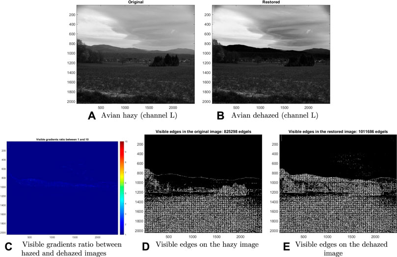
FIGURE 7. Visualizations of the output from the Hautière et al. (2011) metrics, applied on the sensor band L of the avian sensitivity.

In Tables 2, 3, we can observe the results on the different spectral bands. About UV-A sensitive systems, the quantity of reconstructed edges is huge, and the results on e are very different from for the visible. A part of this increase in edges can relate to the use of a guided filter along the DCP dehazing algorithm, which correct UV images that are more blurry than in the visible.

If we exclude the UV-A bands and the polarization-based method, we see a tendency to have the metrics e and $\bar{r}$ higher at longer wavelengths. This means that the ratios of new visible and invisible edges are higher in this range, suggesting that the DCP fog suppression technique might be more effective for long wavelengths.

For the Cricket and Butterfly, we notice that the metric $\bar{r}$ gives a higher result for the spectral case than for the polarization case. This is also coherent with the FADE results. This suggests that the polarization does not bring advantage for dehazing to those sensors, according to the way we captured the information, the way we perform dehazing, and the metric used. We do not infer any statement on the use the animals might make of the polarization information to improve visibility in haze.

4.3 Discussion

From our observation however, it seems like the increase of spectral channel number or the presence of polarization does not improve dehazing. Two possibilities: i-animals use cognitive models that are very different from the physical models we used to perform dehazing, ii-All the animals considered are having similar capacities to evolve in limited visibility, which is neither certain or easy to demonstrate.

Zebrafish and Butterfly who have spectral bands in shorter wavelengths are performing globally better than others for the metrics used. This might be used in the future but will be compensated by i-the weak magnitude of signal in Blue/UV area, ii-the limited ability of optics to handle this signal, e.g. the blur induced by the optics while handling the signal UV. Moreover, Zebrafish and Butterfly might not provide the best visual results (blue color cast in Scene two for the Zebrafish vs the Avian that gives a more natural looking color image). In addition, the handling of UV channels and short wavelengths would increase the complexity of the imaging systems (noise, integration time, specific optics, etc.). We note that the dichromate systems (Pig and Dog) provide fairly good color images and decent dehazed versions.

Our observations are limited to a technical sensing simulation and two scenes case study. They are also related to only some metrics, that we know are not excellent (El Khoury et al., 2018a). The color version is a very human-centred way to analyse those images. However, for a multispectral sensor, this visualisation technique will provide a good way for image visualization.

About the algorithms, we compared two instances of dehazing methods that are based on different priors, so the comparison might be limited. In particular, for polarization, the airlight is estimated by band, whereas for DCP it is the same for every channel. The way to estimate the airlight is one limiting factor for dehazing algorithms. Also, the use of the physical models based dehazing methods might not provide the best performance. This technical framework can provide a test bed for future alternative solutions and algorithms.

We can say little on how animals really use this information. The method and tool that we presented in this paper could however be beneficial to support research within the field of animal vision.

5 Conclusion

In this work, we capture spectral data from a hazy scene, and compute a radiance image as a basis. We then design an experiment to simulate data captured from bio-inspired simulated sensors, having the spectral and polarization sensitivities of six animals and a process to visualize the data as color images. We extend two dehazing techniques to be applied to images with two to five spectral channels and some varied level of polarization sensing.

The dehazed images are compared based on both a spectral approach and a color approach. The bio-inspired sensors behave very differently both in their nature and in performance. Zebrafish, Butterfly, and Primate sensors seem to provide better dehazing results in our experiment.

Despite of the good performance of the aforementioned sensors, we want to moderate the impact of the observations: i-the statistical significance of the scenes used, in terms of metrics and quantity of test images, ii-the transfer to color images that might also reduce the impact of the number of channels (spectral + polarization), iii-it would be difficult for a manufacturer to create a camera that resemble to Zebrafish or Butterfly visual systems for general purpose. Future technical works should investigate the statistical significance of our observations.

Generally, our evaluation pipeline can be re-used for many other types of image processing beside dehazing (image quality evaluation, saliency detection, object recognition, etc.). Independent parts of this work can also be reused as-is by diverse technical fields (medical imaging, remote sensing, etc.). The extension of the dehazing methods to both spectral bands and polarization will work for many setups. The color visualization framework can be used to look at information as color images from in any spectral acquisition.

The research field interested in animal vision might use our proposed framework to verify or validate some hypotheses related to animal vision in turbid media. The impact of this work on ecological or physiological sciences is yet to be discussed with domain experts.

Data Availability Statement

The simulated spectral data is provided online (Lapray, 2021).

Author Contributions

Conceptualization, JT, IF, and PL; Data curation, PL; Formal analysis, IF, JT and PL; Methodology, IF, JT and PL; Software, PL; Validation, PL, JT. and IF; Writing, review and editing, PL, JT. and IF. All authors have read and agreed to the published version of the manuscript.

Funding

This work was supported by the ANR JCJC SPIASI project, grant number ANR-18-CE10-0005 of the French Agence Nationale de la Recherche, and by the Research Council of Norway over the project “Individualized Color Vision-based Image Optimization,” grant number 287 209.

Conflict of Interest

The authors declare that the research was conducted in the absence of any commercial or financial relationships that could be construed as a potential conflict of interest.

Publisher’s Note

All claims expressed in this article are solely those of the authors and do not necessarily represent those of their affiliated organizations, or those of the publisher, the editors, and the reviewers. Any product that may be evaluated in this article, or claim that may be made by its manufacturer, is not guaranteed or endorsed by the publisher.

Acknowledgments

The authors want to thank Joël Lambert for the design and manufacture of the camera mount.

References

Ancuti, C. O., Ancuti, C., Timofte, R., and De Vleeschouwer, C. (2018). “O-haze: a Dehazing Benchmark with Real Hazy and Haze-free Outdoor Images,” in Proceedings of the IEEE conference on computer vision and pattern recognition workshops, Salt Lake City, UT, June 18–22, 2018, 754–762. doi:10.1109/cvprw.2018.00119

CrossRef Full Text | Google Scholar

Ancuti, C., Ancuti, C. O., Timofte, R., and De Vleeschouwer, C. (2018). “I-haze: a Dehazing Benchmark with Real Hazy and Haze-free Indoor Images,” in International Conference on Advanced Concepts for Intelligent Vision Systems, Poitiers, France, 24–27 September (Springer), 620–631. doi:10.1007/978-3-030-01449-0_52

CrossRef Full Text | Google Scholar

Ancuti, C. O., Ancuti, C., Sbert, M., and Timofte, R. (2019). “Dense-haze: A Benchmark for Image Dehazing with Dense-Haze and Haze-free Images,” in 2019 IEEE International Conference on Image Processing (ICIP), Taipei, Taiwan, September 22–25, 2019, 1014–1018. doi:10.1109/icip.2019.8803046

CrossRef Full Text | Google Scholar

Ancuti, C. O., Ancuti, C., and Timofte, R. (2020). “Nh-haze: An Image Dehazing Benchmark with Non-homogeneous Hazy and Haze-free Images,” in Proceedings of the IEEE/CVF Conference on Computer Vision and Pattern Recognition Workshops, Seattle, WA, June 14–19, 2020, 444–445. doi:10.1109/cvprw50498.2020.00230

CrossRef Full Text | Google Scholar

Barta, A., and Horváth, G. (2004). Why Is it Advantageous for Animals to Detect Celestial Polarization in the Ultraviolet? Skylight Polarization under Clouds and Canopies Is Strongest in the Uv. J. Theor. Biol. 226 (4), 429–437. doi:10.1016/j.jtbi.2003.09.017

CrossRef Full Text | Google Scholar

Bay, H., Tuytelaars, T., and Van Gool, L. (2006). “Surf: Speeded up Robust Features,” in European conference on computer vision, Graz, Austria, May 7–13 (Springer), 404–417.

CrossRef Full Text | Google Scholar

Beltran, W. A., Cideciyan, A. V., Guziewicz, K. E., Iwabe, S., Swider, M., Scott, E. M., et al. (2014). Canine Retina Has a Primate Fovea-like Bouquet of Cone Photoreceptors Which Is Affected by Inherited Macular Degenerations. PloS one 9 (3), e90390. doi:10.1371/journal.pone.0090390

PubMed Abstract | CrossRef Full Text | Google Scholar

Bowmaker, J. K., and Dartnall, H. J. (1980). Visual Pigments of Rods and Cones in a Human Retina. J. Physiol. 298 (1), 501–511. doi:10.1113/jphysiol.1980.sp013097

CrossRef Full Text | Google Scholar

Cai, B., Xu, X., Jia, K., Qing, C., and Tao, D. (2016). Dehazenet: An End-To-End System for Single Image Haze Removal. IEEE Trans. Image Process. 25 (11), 5187–5198. doi:10.1109/tip.2016.2598681

PubMed Abstract | CrossRef Full Text | Google Scholar

Choi, L. K., and You, J., and (2015). Referenceless Prediction of Perceptual Fog Density and Perceptual Image Defogging. IEEE Trans. Image Process. 24 (11), 3888–3901. doi:10.1109/tip.2015.2456502

PubMed Abstract | CrossRef Full Text | Google Scholar

El Khoury, J., Thomas, J-B., and Mansouri, A. (2014). “Does Dehazing Model Preserve Color Information,” in 2014 Tenth International Conference on Signal-Image Technology and Internet-Based Systems, Marrakech, Morocco, November 23–27, 606–613.

CrossRef Full Text | Google Scholar

El Khoury, J., Moan, S. L., Thomas, J.-B., and Mansouri, A. (2018). Color and Sharpness Assessment of Single Image Dehazing. Multimed Tools Appl. 77 (12), 15409–15430. doi:10.1007/s11042-017-5122-y

CrossRef Full Text | Google Scholar

El Khoury, J., Thomas, J.-B., and Mansouri, A. (2018). A Database with Reference for Image Dehazing Evaluation. J Imaging Sci. Technol. 62 (1), 105031–1050313. doi:10.2352/j.imagingsci.technol.2018.62.1.010503

CrossRef Full Text | Google Scholar

El Khoury, J., Thomas, J.-B., and Mansouri, A. (2020). “A Spectral Hazy Image Database,” in Image and Signal Processing. Editors A El Moataz, D. Mammass, A Mansouri, and F. Nouboud (Springer International Publishing), 44–53. doi:10.1007/978-3-030-51935-3_5

CrossRef Full Text | Google Scholar

Endeman, D., Klaassen, L. J., and Kamermans, M. (2013). Action Spectra of Zebrafish Cone Photoreceptors. PLoS One 8 (7), e68540. doi:10.1371/journal.pone.0068540

PubMed Abstract | CrossRef Full Text | Google Scholar

Guild, J., and Petavel, J. E. (1931). The Colorimetric Properties of the Spectrum. Philos. Trans. R. Soc. Lond. Ser. A, Contain. Pap. a Math. or Phys. Char. 230 (681-693), 149–187.

Google Scholar

Hart, N. S., and Vorobyev, M. (2005). Modelling Oil Droplet Absorption Spectra and Spectral Sensitivities of Bird Cone Photoreceptors. J. Comp. Physiol. A. 191 (4), 381–392. doi:10.1007/s00359-004-0595-3

CrossRef Full Text | Google Scholar

Hautière, N., Tarel, J.-P., Aubert, D., and Dumont, É. (2011). Blind Contrast Enhancement Assessment by Gradient Ratioing at Visible Edges. Image Anal. Stereol. 27 (2), 87–95. doi:10.5566/ias.v27.p87-95

CrossRef Full Text | Google Scholar

He, K., Sun, J., and Tang, X. (2011). Single Image Haze Removal Using Dark Channel Prior. IEEE Trans. Pattern Anal. Mach. Intell. 33 (12), 2341–2353. doi:10.1109/tpami.2010.168

PubMed Abstract | CrossRef Full Text | Google Scholar

He, K., Sun, J., and Tang, X. (2013). Guided Image Filtering. IEEE Trans. Pattern Anal. Mach. Intell. 35 (6), 1397–1409. doi:10.1109/tpami.2012.213

PubMed Abstract | CrossRef Full Text | Google Scholar

Herzmann, D., and Labhart, T. (1989). Spectral Sensitivity and Absolute Threshold of Polarization Vision in Crickets: a Behavioral Study. J. Comp. Physiol. 165 (3), 315–319. doi:10.1007/bf00619350

CrossRef Full Text | Google Scholar

Horváth, G., Gál, J., Labhart, T., and Wehner, R. (2002). Does Reflection Polarization by Plants Influence Colour Perception in Insects? Polarimetric Measurements Applied to a Polarization-Sensitive Model Retina of papilio Butterflies. J. Exp. Biol. 205 (21), 3281–3298.

Google Scholar

Horváth, G., Lerner, A., and Shashar, N. (2014). Polarized Light and Polarization Vision in Animal Sciences, Vol. 2. Berlin: Springer.

Google Scholar

Kasparson, A. A., Badridze, J., and Maximov, V. V. (2013). Colour Cues Proved to Be More Informative for Dogs Than Brightness. Proc. R. Soc. B. 280 (1766), 20131356. doi:10.1098/rspb.2013.1356

PubMed Abstract | CrossRef Full Text | Google Scholar

Koschmeider, H. (1924). Theorie der horizontalen sichtweite. Beitrage zur Physik der freien Atmosphare, 33–53.

Google Scholar

Lapray, P. J., Thomas, J-B., and Gouton, P. (2017). High Dynamic Range Spectral Imaging Pipeline for Multispectral Filter Array Cameras. Sensors (Basel) 17 (6), 1281. doi:10.3390/s17061281

PubMed Abstract | CrossRef Full Text | Google Scholar

Lapray, P-J., Gendre, L., Foulonneau, A., and Bigué, L. (2018). “Database of Polarimetric and Multispectral Images in the Visible and Nir Regions,” in Unconventional Optical Imaging (International Society for Optics and Photonics), Vol. 10677, 1067738.

CrossRef Full Text | Google Scholar

Lapray, P.-J., Thomas, J.-B., and Farup, I. (2021). Simulated data: Bio-inspired multimodal imaging in reduced visibility. doi:10.6084/m9.figshare.14854170.v1

CrossRef Full Text

Li, B., Peng, X., Wang, Z., Xu, J., and Feng, D. (2017). “Aod-net: All-In-One Dehazing Network,” in 2017 IEEE International Conference on Computer Vision (ICCV), Venice, Italy, October 22–29, 2017, 4780–4788. doi:10.1109/iccv.2017.511

CrossRef Full Text | Google Scholar

Li, R., Pan, J., Li, Z., and Tang, J. (2018). “Single Image Dehazing via Conditional Generative Adversarial Network,” in Proceedings of the IEEE Conference on Computer Vision and Pattern Recognition (CVPR), Salt Lake City, UT, June 18–23, 2018. doi:10.1109/cvpr.2018.00856

CrossRef Full Text | Google Scholar

Maloney, L. T., and Wandell, B. A. (1986). Color Constancy: a Method for Recovering Surface Spectral Reflectance. J. Opt. Soc. Am. A. 3 (1), 29–33. doi:10.1364/josaa.3.000029

CrossRef Full Text | Google Scholar

Martínez-Domingo, M. Á., Valero, E. M., Nieves, J. L., Molina-Fuentes, P. J., Romero, J., and Hernández-Andrés, J. (2020). Single Image Dehazing Algorithm Analysis with Hyperspectral Images in the Visible Range. Sensors 20 (22), 6690. doi:10.3390/s20226690

CrossRef Full Text | Google Scholar

Morimatsu, M., Monno, Y., Tanaka, M., and Okutomi, M. (2020). “Monochrome and Color Polarization Demosaicking Using Edge-Aware Residual Interpolation,” in 2020 IEEE International Conference on Image Processing (ICIP), Abu Dhabi, United Arab Emirates, October 25–28, 2020, 2571–2575. doi:10.1109/icip40778.2020.9191085

CrossRef Full Text | Google Scholar

Paul, E. (1997). “Debevec and Jitendra Malik. Recovering High Dynamic Range Radiance Maps from Photographs,” in Proceedings of the 24th Annual Conference on Computer Graphics and Interactive Techniques, SIGGRAPH ’97, Los Angeles, CA, August 3–8, 1997 (USA: ACM Press/Addison-Wesley Publishing Co), 369–378.

Google Scholar

Schechner, Y. Y., Narasimhan, S. G., and Nayar, S. K. (2003). Polarization-based Vision through Haze. Appl. Opt. 42 (3), 511–525. doi:10.1364/ao.42.000511

PubMed Abstract | CrossRef Full Text | Google Scholar

Standard (1999). Multimedia Systems and Equipment - Colour Measurement and Management - Part 2-1: Colour Management - Default Rgb Colour Space - Srgb. Geneva, CH: International Electrotechnical Commission.

Google Scholar

Von Frisch, K. (2013). The Dance Language and Orientation of Bees. Cambridge, Mass: Harvard University Press.

Google Scholar

Wright, W. D. (1929). A Re-determination of the Trichromatic Coefficients of the Spectral Colours. Trans. Opt. Soc. 30 (4), 141–164. doi:10.1088/1475-4878/30/4/301

CrossRef Full Text | Google Scholar