- 1Center for Vision Technologies, SRI International, Menlo Park, CA, United States
- 2Center for Education Research and Innovation, SRI International, Menlo Park, CA, United States
Early development of specific skills can help students succeed in fields like Science, Technology, Engineering and Mathematics. Different education standards consider “Collaboration” as a required and necessary skill that can help students excel in these fields. Instruction-based methods is the most common approach, adopted by teachers to instill collaborative skills. However, it is difficult for a single teacher to observe multiple student groups and provide constructive feedback to each student. With growing student population and limited teaching staff, this problem seems unlikely to go away. Development of machine-learning-based automated systems for student group collaboration assessment and feedback can help address this problem. Building upon our previous work, in this paper, we propose simple CNN deep-learning models that take in spatio-temporal representations of individual student roles and behavior annotations as input for group collaboration assessment. The trained classification models are further used to develop an automated recommendation system to provide individual-level or group-level feedback. The recommendation system suggests different roles each student in the group could have assumed that would facilitate better overall group collaboration. To the best of our knowledge, we are the first to develop such a feedback system. We also list the different challenges faced when working with the annotation data and describe the approaches we used to address those challenges.
1 Introduction
Both the Next Generation Science Standards (States, 2013) and the Common Core State Standards (Daggett and GendroO, 2010) consider “Collaboration” to be a crucial skill, that is needed to be inculcated in students early on for them to excel in fields like Science, Technology, Engineering and Mathematics (STEM). To instill collaborative skills, instructional methods like project-based learning (Krajcik and Blumenfeld, 2006) or problem-based learning (Davidson and Major, 2014) are the most common approaches adopted by teachers in K-12 classrooms. However, it can be hard for teachers to identify specific behavioral cues that contribute to or detract from the collaboration effort (Taggar and Brown, 2001; Loughry et al., 2007; Smith-Jentsch et al., 2008). Also, with growing classroom sizes, monitoring and providing feedback to individual students can be very difficult. One can mitigate these issues by using machine-learning to develop systems that automatically assess student group collaboration (Soller et al., 2002; Talavera and Gaudioso, 2004; Anaya and Boticario, 2011; Genolini and Falissard, 2011; Spikol et al., 2017; Guo and Barmaki, 2019; Huang et al., 2019; Kang et al., 2019; Reilly and Schneider, 2019; Alexandron et al., 2019; Vrzakova et al., 2020).
In our previous work we designed a Collaboration Conceptual Model (CCM) that provides an automated assessment of the collaboration quality of student groups based on their behavioral communication at individual and group levels (Alozie et al., 2020a,b). CCM represents a multi-level, multi-modal integrated behavior analysis tool and is illustrated in Figure 1. Audio and video recordings of a student group performing a collaborative task is passed as input to this model. Next, low level features like facial expressions, body-pose are extracted at Level E. Information like joint attention and engagement are encoded at Level D. Level C describes complex interactions and individual behaviors. Level B is divided into two categories: Level B1 describes the overall group dynamics for a given task; Level B2 describes the changing individual roles assumed by each student in the group. Finally, Level A describes the overall collaborative quality of the group based on the information from all previous levels. In this paper, we focus on developing deep-learning models that map spatio-temporal representations from Level B2 → Level A and Level C → Level A, as indicated by the red arrows.
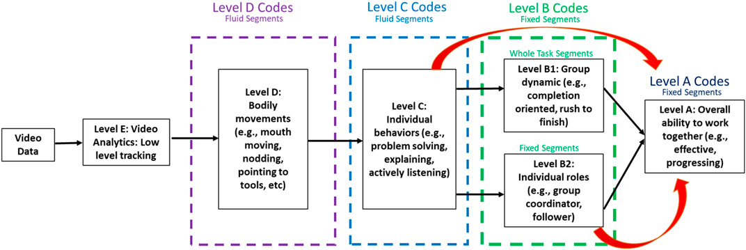
FIGURE 1. The collaboration conceptual model. This illustration was first described in (Som et al., 2020).
Using this conceptual model as a reference, in a different paper (Som et al., 2020) we developed simple Multi Layer Perceptron (MLP) deep-learning models that predict a student group’s collaboration quality (Level A) from individual student roles (Level B2) and behaviors (Level C), indicated by the red arrows in Figure 1. These MLP models take simple histogram representations as input. While these simple representations and models were sufficient for observing good classification performance, what they lacked was explainability. When developing such automated systems, one should focus not only on performance but also make the model more easily explainable and interpretable. We addressed this to some extent in another paper (Som et al., 2021), where we used temporal representations of student roles along with simple 1D ResNet deep-learning models (Wang et al., 2017). This setup allowed us to use Grad-CAM (Selvaraju et al., 2017) visualizations that help point to important temporal instances in the task that contribute towards the model’s decision.
In this paper, we add another level of detail and explore the effectiveness of spatio-temporal representations of student role and behavior annotations for estimating group collaboration quality. We model these representations using simple 2D CNN models. In addition to identifying important temporal instances, this setup allows us to localize important subsets of students in the group. This level of detail is crucial for developing an automated recommendation system. Our proposed recommendation system offers individual-level and group-level recommendations. However, when developing the collaboration assessment and feedback systems we did encounter challenges like limited and imbalanced training data, as seen from the distribution of Level A codes in Figure 2. Here, Level A represents the label space for training our collaboration quality assessment models. Also, the annotations for levels A, B2 and C were collected in two different modality settings: Video (no audio) and Audio + Video. We wanted to check if visual behavioral cues alone could be used to estimate collaborative skills. However, in our previous work (Som et al., 2020), we observed significant differences in classification performance between the two modality settings, with the Video modality annotations performing more poorly than Audio + Video annotations. In this paper, we go through the approaches introduced in our previous work to address the above challenges and limitations. We also discuss ways in which we reduce the performance gap between the two modality settings. The main contributions in this paper are summarized below.
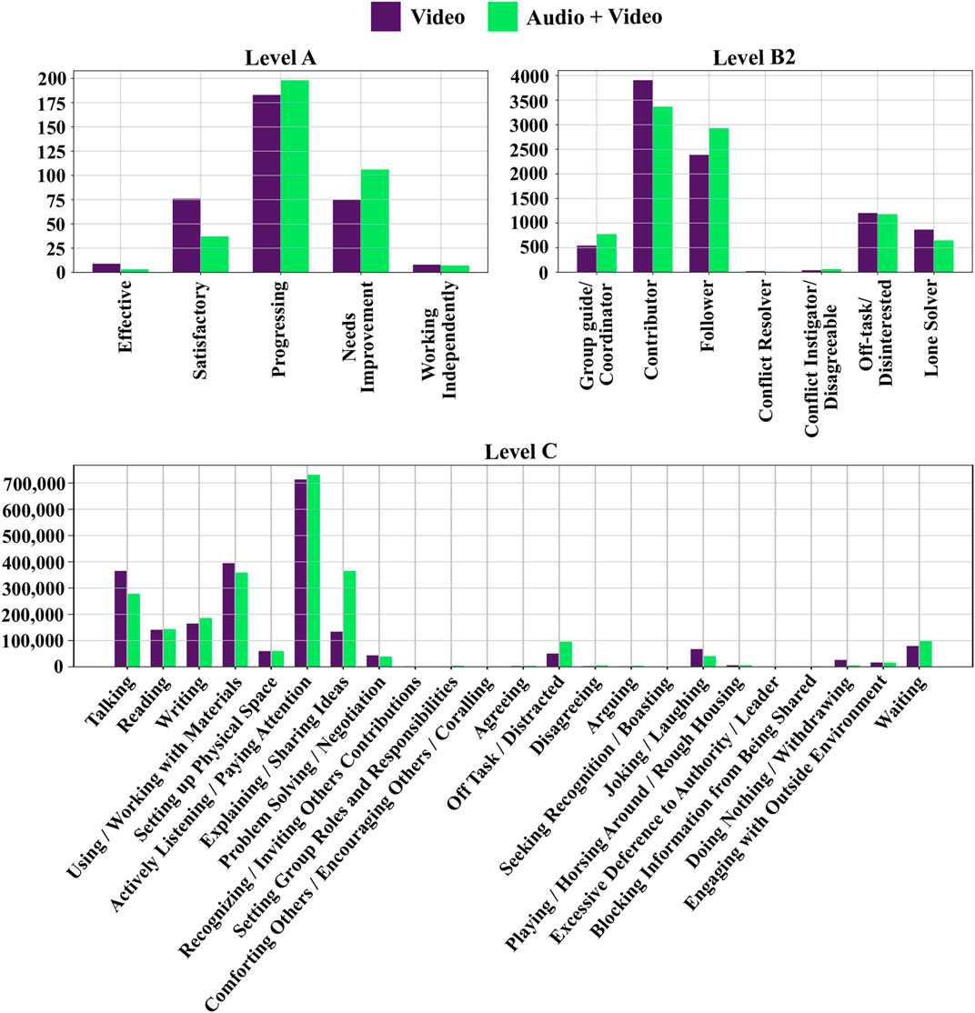
FIGURE 2. Distribution of codes for levels A, B2 and C. Note, Level A was coded over each task. Level B2 codes were created over 1 minute time segments. Level C codes were coded using fluid length segments and the distribution shown here was created by sampling at every 0.1 seconds. The distribution of Level A codes was first illustrated in (Som et al., 2020).
1.1 Contributions
• We exploit the ordered nature of the label space (i.e., Level A) and use the Ordinal-Cross-Entropy loss function, which imposes a higher penalty on misclassified samples during the training process. The benefits of this loss function were initially discussed in (Som et al., 2020).
• We address the limited and imbalanced training data challenges by using a controlled variant of Mixup data augmentation. Mixup is a simple approach for generating additional synthetic data samples for training the deep-learning model (Zhang et al., 2018). The controlled Mixup augmentation variant was also initially introduced in the following paper (Som et al., 2020).
• For the collaboration assessment classification system, we propose using a spatio-temporal representation of the annotation data along with simple 2D CNN models to enable better localization of important temporal instances and student interactions.
• The nature of the spatio-temporal representations allows us to create more variations in our training dataset by permuting the order of the students in the group. For example, each group in our dataset has a maximum of 5 students. This implies that we can make 120 variations/permutations from one spatio-temporal representation. This allows us to increase the size of the original dataset by 120 times.
• We discuss our thoughts and empirical observations for reducing the performance gap between the Video and Audio + Video modality settings.
• The spatio-temporal representations and the 2D CNN models trained for collaboration quality assessment are used for developing the proposed recommendation system. We use a simple gradient-descent optimization framework for designing the recommendation system. It is capable of providing group level or individual student level recommendations. To the best of our knowledge, we are the first to propose such a recommendation system that focuses on improving group collaboration quality.
1.2 Paper Outline
Section 2 discusses related work. Section 3 provides necessary background on the different loss functions and mixup augmentation. Section 4 describes the dataset, the different features extracted for Levels B2 and C, and the approach for generating synthetic spatio-temporal samples using a controlled variant of Mixup augmentation. Section 5 describes the experiments and results. Section 6 concludes the paper.
2 Related Work
There have been several recent works that explore using machine-learning concepts for collaboration problem-solving, analysis and assessment. For example, Reilly et al. used Coh-Metrix indices (a natural language processing tool to measure cohesion for written/spoken texts) to train machine-learning models to classify co-located participant discourse in a multi-modal learning analytics study (Reilly and Schneider, 2019). Their multi-modal dataset contained eye-tracking, physiological and motion sensing data. Their study only had two collaboration quality states and focused on evaluating the level of cooperation between novice programmers that were instructed to program a robot. Using the same dataset, Huang et al. used an unsupervised machine learning approach to discover unproductive collaborative states (Huang et al., 2019). They were able to develop a three-state solution that showed high correlation with task performance, collaboration quality and learning gain. Kang et al. also used an unsupervised learning approach to study the collaborative problem-solving process of middle school students (Kang et al., 2019). They analyzed data collected using a computer-based learning environment of student groups playing a serious game. For their analysis they employed KmL, an R package for applying k-means clustering on longitudinal data (Genolini and Falissard, 2011). They too identified three different states using the proposed unsupervised method. There are different layers of collaboration that range from individual behaviors to group dynamics to overall ability to work interdependently. The codes defined for Level A in our CCM model describe the “Overall ability to work together interdependently”. From different theories on collaboration, we derived five codes or collaboration quality states that help describe how groups tend to work together (Alozie et al., 2020a,b). The five Level A codes are effective, satisfactory, progressing, needs improvement and working independently. They are used as the target label categories in a supervised learning setup in this paper.
Other prior works include—Talavera and Gaudioso utilized clustering methods to discover and characterize similar user behaviors in unstructured collaboration spaces (Talavera and Gaudioso, 2004). Spikol et al. suggested using tools from multimodal learning analytics (MMLA) to gain insights into what happens when students are engaged in collaborative, project-based learning activities (Spikol et al., 2017). Soller et al. proposed using Hidden Markov Models (HMM) to analyze and understand how group members in an on-line knowledge sharing conversation share, assimilate and build knowledge together (Soller et al., 2002). Anaya and Boticario explored unsupervised and supervised approaches to evaluate 12 quantitative statistical indicators of student interactions in a forum (Anaya and Boticario, 2011). However, as mentioned by them, their proposed indicators do not have any semantic information of the message contents. For on-line collaborative tasks, Vrzakova et al. examined unimodal data recordings (like screen activity, speech and body movements) and respective multimodal combinations, and tried correlating them with task performance (Vrzakova et al., 2020).
Guo and Barmaki used a deep-learning based object detection approach for analysis of pairs of students collaborating to locate and paint specific body muscles on each other (Guo and Barmaki, 2019). They used a Mask R-CNN for detecting the students in the video recordings. They claim that close proximity of group participants and longer time taken to complete a task are indicators of good collaboration. However, they quantify participant proximity by the percentage of overlap between the student masks obtained using the Mask R-CNN. The amount of overlap can change dramatically across different view points. Also, collaboration need not necessarily be exhibited by groups that take a longer time to complete a task. In this paper, the deep-learning models are based on the systematically designed multi-level collaboration conceptual model shown in Figure 1.
3 Background
3.1 Cross-Entropy Loss Functions
The categorical-cross-entropy loss is the most common loss function used to train deep-learning models. For a C-class classification problem, let the input variables or feature representation be denoted as x, ground-truth label vector as y and the predicted probability distribution as p. Given a training sample (x, y), the categorical-cross-entropy (CE) loss is simply defined as
Here, pi represents the predicted probability of the i-th class. Here, ∑iyi = ∑ipi = 1, with both y and p representing vectors of length C. For imbalanced datasets, the categorical-cross-entropy loss causes the learnt weights of the model to be biased towards classes with more number of samples in the training set. Also, if the label space of the dataset exhibits an ordered structure, the categorical-cross-entropy loss will only focus on the predicted probability of the ground-truth class. It ignores how far off the incorrectly predicted sample actually is from the ground-truth label. These limitations can be addressed to some extent by using the ordinal-cross-entropy (OCE) loss function (Som et al., 2020), defined in Equation 2.
Here, (1 + w) represents the weighting variable, argmax returns the index of the maximum valued element and |.| returns the absolute value. When training the model, w = 0 for correctly classified training samples, with the ordinal-cross-entropy loss behaving exactly like the categorical-cross-entropy loss. However, for misclassified samples the ordinal-cross-entropy loss will return a higher loss value. The increase in loss is proportional to how far away a sample is misclassified from its ground-truth class label. In our previous works (Som et al., 2020; Som et al., 2021) we found the higher loss penalization helps improve the overall classification performance of the model.
3.2 Mixup Data Augmentation
Class imbalance is a very common issue in most naturally occurring datasets. For a classification problem, it refers to the unequal representation or occurrence of samples in different class label categories. This can happen despite best data collection practices. If not appropriately addressed it can result in unwanted biases creeping into the machine learning model. For example, if the training dataset used to train the machine learning model is more representative of some label categories, then the model’s prediction would systematically be worse for the under-represented categories. Conversely, over-representation of certain classes can skew the decision towards a particular result. Mixup augmentation is a simple technique that can be used for imbalanced datasets (Zhang et al., 2018). Mixup helps generate additional synthetic training samples and encourages the machine-learning model to behave linearly in-between the different label categories. It extends the training distribution by incorporating the prior knowledge that linear interpolations of input variables x should lead to linear interpolations of the corresponding target labels y. Consider the following example, let (x1, y1) and (x2, y2), represent two random training samples in our imbalanced dataset. We can create additional samples from these two samples by linearly combining the input variables and their corresponding class labels, as illustrated in Eq. (3).
Here,

FIGURE 3. Beta(α,α) distributions for α = 0.1, 0.4, 0.7, 1.0 respectively. Each Beta distribution plot has a different y-axis range and represents a 500-bin histogram of 200,000 randomly sampled λs. Note, most λs for Beta(0.1,0.1) are at 0 and 1. This illustration was first described in (Som et al., 2020).
4 Dataset Description, Feature Extraction and Synthetic Data Generation
4.1 Dataset Description and Analysis
Audio and video data recordings were collected from 15 student groups, across five middle schools. Amongst these groups, 13 groups had four student participants, one group had three students, and one group had five students. The student participants first completed a brief survey to collect information like demographic profile, languages spoken, ethnicity and comfort levels with different science concepts. Each group was given the objective of completing 12 open-ended life science and physical science tasks in 1 hour, requiring them to construct models of different science phenomena as a team. Note, each group tried to complete as many tasks possible in the assigned hour. This resulted in 15 hours of audio and video recordings. They received logistic and organization instructions but received no help in group dynamics, group organization, or task completion.
Next, the data recordings were manually annotated by education researchers at SRI International. For the rest of the paper we will refer to them as coders/annotators. In the hierarchical CCM model (Alozie et al., 2020a,b), we refer to the collaboration quality annotations as Level A, individual student role annotations as Level B2 and individual student behaviors as Level C. The coding rubric for these three levels is described in Table 1. Level A codes were assigned over each task, i.e. each task was coded using one Level A code which indicated the overall collaboration quality of the group. Level B2 codes were assigned over 1 minute long segments, and Level C codes were assigned over fluid-length segments. A primary and secondary code was assigned for Level C, while making sure that the coder always assigned at least the primary code. This was done because a student could exhibit either one or multiple simultaneous behaviors when carrying out the task. Next, Levels A and B2 were coded by three annotators. However, Level C was carefully coded by just one annotator. Levels A and B2 were annotated by three annotators to provide variety in group level behavioral characterizations. Both these levels require a higher level of inference, and we confirmed the interpretation of overall group quality assessment and student role identification with a majority decision (more details about this in the following paragraphs). However, Level C requires less inference and the annotators can identify demonstrable interactions and behaviors more easily. When annotators were trained to obtain inter-rater reliability (IRR), the low inference nature of Level C allowed for just one annotator. Also, all annotations created went through a quality checking process to make sure that the annotators maintained reliability throughout the annotation process. The annotators first manually coded each level for the Video modality and later coded the same task for the Audio + Video modality. This was done to prevent any coding bias resulting due to the difference in modalities. They used ELAN (an open-source annotation software) to annotate (Wittenburg et al., 2006). A total of 117 tasks were coded by each annotator, with the duration of each task ranging from 5 to 24 minutes.

TABLE 1. Coding rubric for levels A, B2 and C. The coding rubric for levels B2 and C was first discussed in (Som et al., 2020).
The frequency of the different codes at each level can be seen in Figure 2. Differences in the occurrence of certain codes across the two modality settings can be directly attributed to the availability/lack of auditory information at the time of coding. Moderate-agreement was observed across the coders as seen from the IRR measurements in Table 2. The table doesn’t show IRR for Level C as we only had one coder at this level. Notice that the IRR measurements are very similar across the two modality settings. However, the IRR measurement is always greater in the Audio + Video modality setting. Note, we consider moderate-agreement at Level B2 to be good as it implies that there is sufficient variability in the codes/annotations observed at this level. This allowed us to treat the Level B2 codes provided by each of the three annotators as separate, independent data points. If the coders were in perfect-agreement then there would less observed variations which would have forced us to discard several data instances as we could get away by using the codes from just one coder.
The relationship across the different levels can be easily visualized using co-occurrence matrices and is shown in Figure 4. A co-occurrence matrix allows us to visualize codes at levels B2/C that frequently occur for each code in Level A. These visualizations can help us understand the type of patterns the machine-learning model could potentially end up learning in order to differentiate the different Level A classes. We notice very subtle differences across the two modality settings for the A-B2 co-occurrence matrix. However, we see greater differences in the case of the A-C co-occurrence matrix. In Section 5 we will see how these difference impact the overall performance of the different deep-learning models.
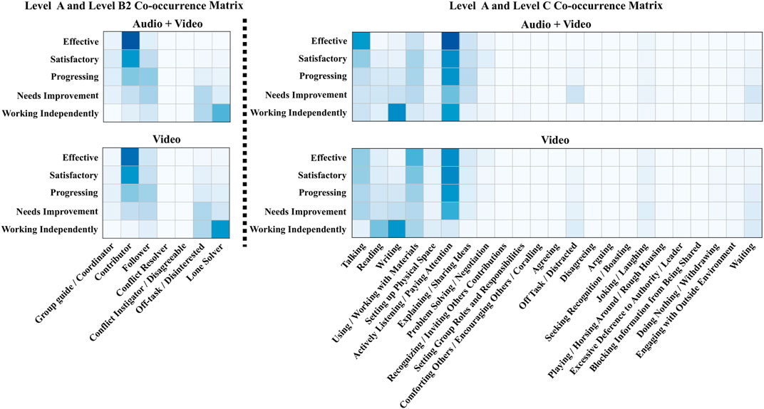
FIGURE 4. Co-occurrence matrix visualization between Level A and Level B2; Level A and Level C, for the two modality settings.
Recall that Level A codes represent the target label categories for our classification problem. To determine the ground-truth Level A code, the majority vote (code) across the three annotators was used as the ground-truth. For cases where a clear majority was not possible, we used the median of the three codes as the ground-truth, based on the ordering depicted in Table 1. For example, if the three coders assigned Satisfactory, Progressing, Needs Improvement for the same task then Progressing would be used as the ground-truth label. Note, we did not observe a majority Level A code for only two tasks in each modality setting. For learning mappings from Level B2 → Level A we had access to only 351 data samples (117 tasks × 3 coders). However, we only had access to 117 data samples (117 tasks coded) for training the machine learning models to learn mappings from Level C → Level A. This makes it an even more challenging classification problem. However, we address the limited data issue by permuting the order of the students and by using the controlled variant of Mixup augmentation. These are discussed in more detail in Section 4.2.3 and Section 4.3.
4.2 Feature Extraction
In this section we go over the evolution of the different feature representation types extracted from our dataset. We start with the simple histogram representation that was discussed in (Som et al., 2020), followed by the temporal representation that was introduced in (Som et al., 2021). Next, we discuss how these two representation types influenced our decision to explore spatio-temporal representations. Finally, we end this section by describing how to increase and balance out the training dataset by permuting the student order in the spatio-temporal representation and using the controlled variant of Mixup augmentation.
4.2.1 Histogram Representation
As mentioned earlier, Level B2 was coded using fixed-length 1 minute segments and Level C was coded using variable-length segments. This is illustrated in Figure 5. A simple yet effective way to summarize and represent all the information in the task is by generating histogram representations of all the codes observed during the task. Figure 5 illustrates the histogram generation process. We first described this process in the following paper (Som et al., 2020). It is quite straightforward to generate histograms for Level B2. However, in the case of Level C we compile all the codes observed after every 0.1 seconds for generating the histogram. Once the histogram is computed we normalize it by the total number of codes observed in the histogram. Normalizing helps remove the temporal aspect associated with the task. For example, if one group took 10 minutes to finish a task and another group took 30 minutes to solve the same task, and both groups were assigned the same Level A code despite the first group having finished the task sooner. The raw histogram representations of both these groups would seem different due to the difference in number of coded segments. However, the normalized histograms would make them more easier to compare.

FIGURE 5. Histogram feature generation for Level B2 and Level C. Different colors indicate different codes assigned to each segment. A B2 histogram was generated for each task by compiling over all the codes, from all the students in the group. Similarly, level C histogram was generated by compiling all the codes, sampled at every 0.1 seconds over the duration of the task. This illustration was first described in (Som et al., 2020).
4.2.2 Temporal Representation
In our dataset, the longest task recorded was little less than 24 minutes long. For this reason we set the maximum length for all tasks to 24 minutes. Due to the fixed-length nature of the segments in Level B2, we assigned an integer value to each B2 code. This means that the seven B2 codes shown in Table 1 were assigned integer values from 1 to 7. The value 0 was used to represent empty segments, i.e., segments that were not assigned a code. For example, in the B2 temporal representation shown in Figure 6, we see a group containing four students that complete a task in 4 minutes. The remaining 20 minutes and the 5th student is assigned a value zero, represented here by the gray colored cells. Thus for each task, the Level B2 temporal feature will have a shape 24 × 5, with 24 representing the number of minutes and 5 representing the number of students in the group.
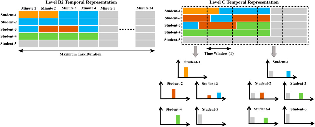
FIGURE 6. Level B2 and Level C temporal representation for a group containing four students. Colored cells represent the different codes listed in Table 1, and the gray cells represent empty or unassigned codes.
We only evaluated Level B2 temporal representations with 1D ResNet models in our previous paper (Som et al., 2021). In this paper we extend our analysis and explore the predictive capabilities of Level C temporal representations. We use 1D ResNet models here as well. However, despite our best efforts it was impossible to directly reuse the process described to generate Level B2 temporal features and use it for Level C. In addition to the variable-length segments, the annotators were instructed to assign a primary and a secondary code for each student. Also, the duration of the assigned primary and secondary codes can be different, further adding to the complexity. To make things simple, we divided the task into fixed-length, non-overlapping time windows of length T. Within each window, we compiled all the primary and secondary codes observed after every 0.1 seconds and computed a histogram representation for each student. This process is similar to the histogram generation process described in the previous section. However, now we generate histograms over fixed-length segments for each student separately. The overall process is clearly illustrated in Figure 6. Finally, we concatenate the generated histograms. Thus, Level C temporal representation consists of dynamically varying set of histograms for each student. In addition to the 23 codes listed in Table 1, we also include an unassigned or empty code for instances when no code was assigned by the annotator, as shown by the gray colored segments in Figure 6. Let us consider the following example: When T = 60 seconds, the Level C temporal feature will have a shape 24 × 120, where 120 corresponds to the 24-bin histogram (23 Level C codes and 1 unassigned/empty code) computed for each of the 5 students and 24 corresponds to the total number of minutes.
4.2.3 Spatio-Temporal Representation
To mitigate the challenges and limitations faced in designing the histogram and temporal representations, in this section we describe the spatio-temporal feature generation process and discuss the benefits that come from this type of representation. As illustrated in Figure 7, the spatio-temporal representation design is inspired from both the histogram and temporal feature generation processes. Its appearance is exactly the same as the Level C temporal feature. However, now we extend this design to Level B2 as well. The 2D representation space allows us to use various 2D CNN deep-learning models that have been carefully designed and validated. Also, this representation makes it easier to generate additional training samples using the controlled Mixup augmentation technique. Mixup augmentation was not possible in the case of B2 temporal features, as we had used integer values to represent each code. The spatio-temporal representation also allows us to generate more data samples by permuting the order of students in the group. This was also possible in the case of the temporal representation but was not explored in our previous paper. Since we observe a maximum of 5 students in our dataset, through permutation we can generate 120 variations/permutations from a single spatio-temporal sample. This alone allows us to increase the size of our dataset by 120 times, without any Mixup augmentation.
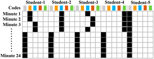
FIGURE 7. Illustration of a spatio-temporal data sample. Black colored cells indicate the code that was assigned to each student during the task. Colored boxes indicate the different codes at levels B2 and C.
The black colored cells in Figure 7 indicate which codes were assigned to each student at every minute in the task. For Level B2 only one code was assigned over fixed-length 1 minute segments. However, for Level C there could be multiple codes observed over the defined period of time (T). With that said, the underlying process to generate the spatio-temporal representation still remains the same for both levels. The only main difference in the case of Level C is that for each student, the histogram computed over time window T is normalized such that all its elements sum to 1. Other than that, all the above mentioned advantages still hold true for both levels B2 and C.
4.3 Controlled Mixup Augmentation
We know that our dataset has an imbalanced label distribution, as seen from the distribution of Level A codes in Figure 2. Conventional Mixup selects a random pair of samples and linearly interpolates them using a λ that is sampled from a Beta distribution. However, this does not help address the class imbalance problem. We want to be able to generate a fixed number of samples for a specific label category. We do this by first limiting the range of λ, i.e., λ ∈ [τ, 1], with τ representing the desired threshold. Figure 8 shows a Beta (0.4,0.4) distribution where we only sample λ above threshold τ. Next, we generate additional samples for a specific class by pairing that class with its adjacent or neighboring classes. Let us use the following denotation: (primary-class, [adjacent-class-1, adjacent-class-2]), where primary-class represents the class for which we want to generate more samples; adjacent-class-1 and adjacent-class-2 represent its immediate class neighbors. Using this convention we create the following pairs: [Effective, (Satisfactory, Progressing)]; [Satisfactory, (Effective, Progressing)]; [Progressing, (Satisfactory, Needs Improvement)]; [Needs Improvement, (Progressing, Working Independently)]; and [Working Independently (Progressing, Needs Improvement)]. The final step involves generating n samples for the primary-class using Mixup. We do this by randomly pairing samples from the primary-class with samples from its adjacent-classes. This process is repeated n times to create n synthetic samples. Note, λ is always multiplied with the primary-class sample and (1—λ) is multiplied with the adjacent-class sample. We used controlled Mixup augmentation for the first time in (Som et al., 2020), where we used it to generate additional samples for the under-represented classes for the histogram representations. Here too we apply controlled Mixup on spatio-temporal representations after increasing the training set by permuting the samples. Here, we set τ = 0.9 and n = 25000.
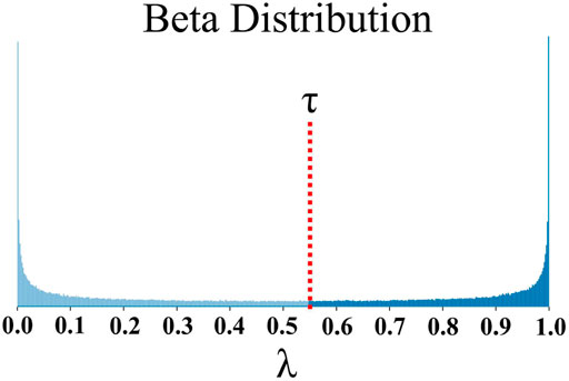
FIGURE 8. Illustration of a Beta(α, α) distribution with α = 0.4. Using Mixup we generate additional data samples, where the λ selected is always above threshold τ.
5 Experiments
5.1 Network Architecture
We used a simple 5-layer Multi Layer Perceptron (MLP) model for the histogram representations and a temporal/1D ResNet model for the temporal representations. Detailed description of the architecture design for these two models can be found in the following papers (Som et al., 2020; Som et al., 2021). The spatio-temporal representation was specifically designed for it to be easily plugged into various 2D CNN models, that have been widely used and validated in other research works. However, in this paper we limited ourselves to a very light and simple 2D CNN architecture design. Our model consists of an input layer that takes in the spatio-temporal representation; one 2D convolution layer containing m filters of shape h × w; one batch-normalization layer; one ReLU activation layer; followed by a global-average-pooling layer and a softmax layer. Filter parameters h, w represent the filter height and width along the temporal (along time) and spatial (across students) axis respectively. Here, w = 5 (# of codes at Level B2/C). We varied m = 1, 6, 24, 96; h = 1, 2, 4, and reported results for the best performing case. The filters were made to stride only along the temporal axis, with the stride-length set to 1. Based on these parameter settings, the number of trainable parameters ranged from 53 to 16133 for B2 spatio-temporal features and 133 to 46853 for C spatio-temporal features. The number of trainable parameters here is significantly smaller than the MLP and ResNet models we explored in our previous studies.
5.1.1 Training and Evaluation Protocol
All models were developed using Keras with TensorFlow backend (Chollet, 2015). We used the Adam optimizer (Kingma and Ba, 2014) with the Ordinal-Cross-Entropy loss function and trained the 2D CNN models for 100 epochs. The batch-size, patience and minimum-learning-rate hyperparameters to 64, 10, and 0.0001 respectively. The learning-rate was reduced by a factor of 0.5 if the loss did not change after a certain number of epochs, indicated by the patience hyperparameter. We saved the best model that gave us the lowest test-loss for each training-test split. We used a round-robin leave-one-group-out cross validation protocol. This means that for our dataset consisting of g student groups, for each training-test split we used data from g—1 groups for training and the left-out group was used as the test set. This was repeated for all g groups and the average result was reported. For our experiments g = 14 though we have temporal representations from 15 student groups. This is because all samples corresponding to the Effective class were found only in one group. Due to this reason and because of our cross-validation protocol we do not see any test samples for the Effective class in the Audio + Video modality setting and for the Working Independently class in the Video setting. We also used the leave-one-group-out protocol for training the MLP and ResNet models. Please refer to the following papers for a detailed description of the different hyperparameter settings used in the MLP and ResNet models (Som et al., 2020; Som et al., 2021). Also, all models were evaluated on the original test set, that was not subjected to any augmentation.
5.2 Performance Comparison Across Different Feature Representations
Here we compare the performance between the 2D CNN, ResNet and MLP models. Based on F1-Score performance, Tables 3 and 4 summarize the best performing models under the different feature-classifier settings for levels B2 and C respectively. The histogram feature results were first presented in Som et al. (2020). The temporal feature results for Level B2 in the Audio + Video modality setting were discussed in Som et al. (2021). In this paper we extend that analysis and show results for Level B2 temporal features in the Video modality setting and Level C temporal features in both modality settings. In the case of Level B2, for both modality settings the F1-Score performance tends to decrease as we go from the histogram representation towards the spatio-temporal representation. This could be attributed to the discrete nature of the data as we try to add more nuanced details to better represent and model Level B2 information. However, we see a different trend in the case of Level C. We notice that Level C temporal features perform significantly better than their histogram and spatio-temporal counterparts. One could expect the temporal and spatio-temporal representations at Level C to show similar performance since the underlying feature generation process is the same. The difference could be attributed to the type of deep-learning model used to model each feature type.
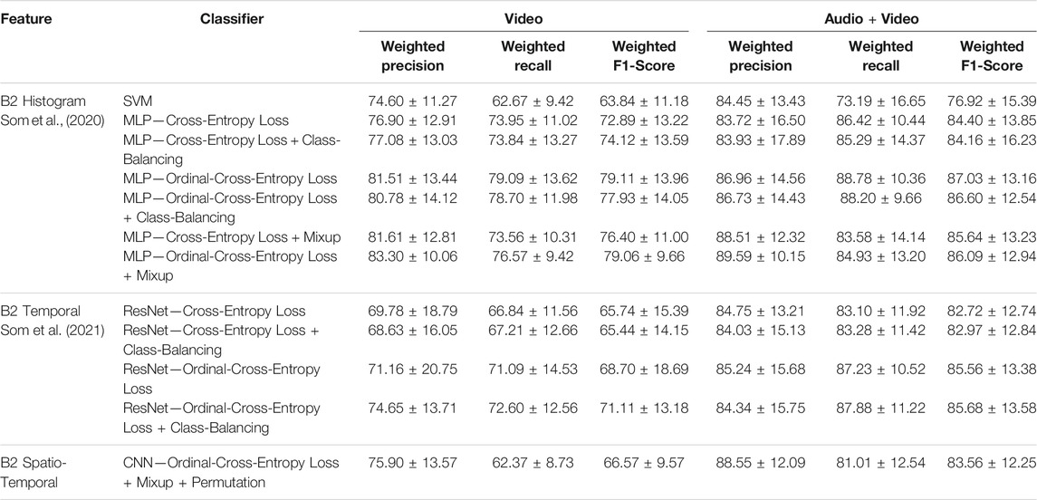
TABLE 3. Weighted precision, weighted recall and weighted F1-score Mean ± Std measurements for the best MLP, ResNet and 2D CNN models under different settings. These models were evaluated on different feature representations extracted for Level B2.
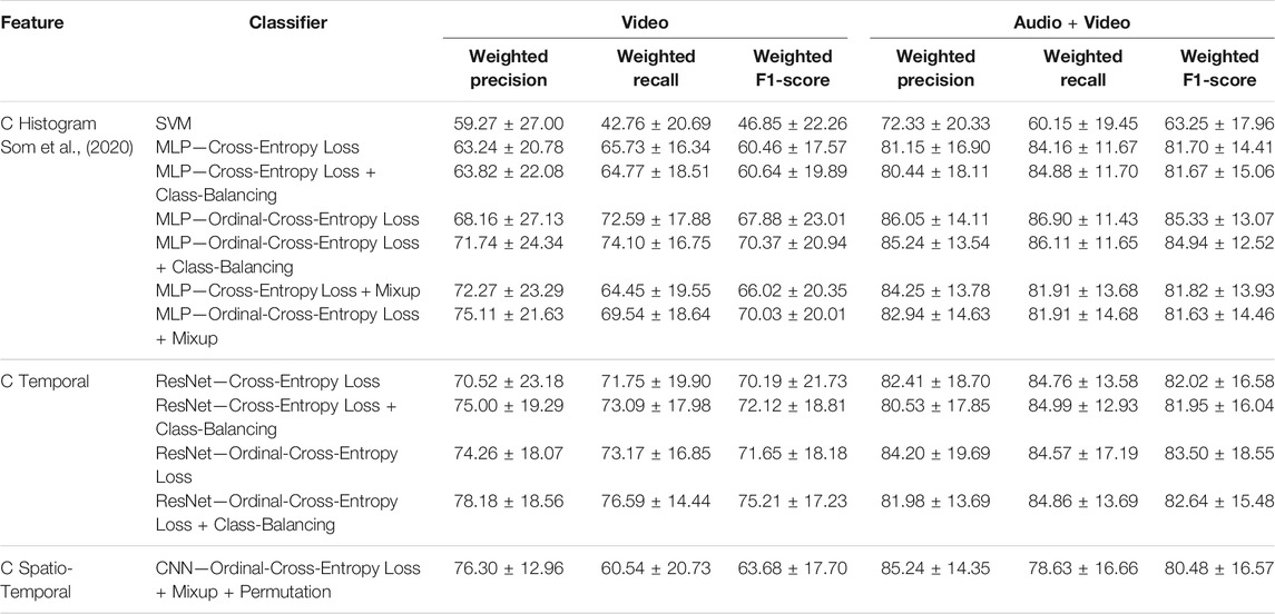
TABLE 4. Weighted precision, weighted recall and weighted F1-score Mean ± Std measurements for the best MLP, ResNet and 2D CNN models under different settings. These models were evaluated on different feature representations extracted for Level C.
Ideally we want high precision and high recall. However, in realistic cases and when working with limited, imbalanced test sets, we should strive for a higher precision than recall. Luckily, our 2D CNN models across both levels exhibit a higher precision that is comparable to or even better than the highest precision MLP and ResNet models. Another thing to note is that our 2D CNN models are one to four orders of magnitude smaller than the ResNet and MLP models used in our previous studies. This is reassuring as it implies that there is still scope for improvement by using more sophisticated 2D architecture models. The reason for using such a small model was two-fold: First, we wanted to quickly check the ability of very simple 2D CNN models in estimating collaboration quality and their utility in the proposed recommendation system design; Second, we wanted to reduce the overall training time. We were able to create a large training set thanks to permuting the students and controlled Mixup augmentation. However, the larger training set resulted in longer training times. Use of more sophisticated models would entail training several thousand or million parameters. This could make the whole training process even slower. Thus, we decided to keep the deep-learning model simple.
5.3 Performance Across Modality Settings
From the summarized result shown in Tables 3 and 4, one can immediately notice the huge difference in classification performance across the two modality settings. This is true irrespective of the level or the representation type. Our initial hypothesis for the lower performance of Video modality features leaned towards the possibility of recording noisy annotations. This could be due to the absence of audio information at the time of coding. Note, annotations for levels A, B2 and C were first created under the Video modality setting and then in the Audio + Video setting. This was done to prevent any coding bias that could result due to the difference in modality conditions. If our hypothesis is true then that would entail that the codes created in the Video setting do not accurately capture events in the Video recording. To test this, we trained our deep-learning models to map features from the Video setting to ground-truth labels in the Audio + Video modality setting. For convenience, we will refer to this setting as the Cross-modal setting. To our surprise, models trained in this protocol showed a significant improvement in their F1-Score classification performance, thereby rejecting our initial hypothesis. Figures 9, 10 compare the F1-Score performance across the Video, Audio + Video and the new Cross-modal setting. Here, H1-H6 represent the different histogram-classifier settings; T1-T4 represent the different temporal-classifier settings; and ST1 represents the spatio-temporal-classifier setting. Except for H5 and H6 in the case of Level B2, in all other cases we observe the Cross-modal setting perform close to and at times better than the Audio + Video modality setting.
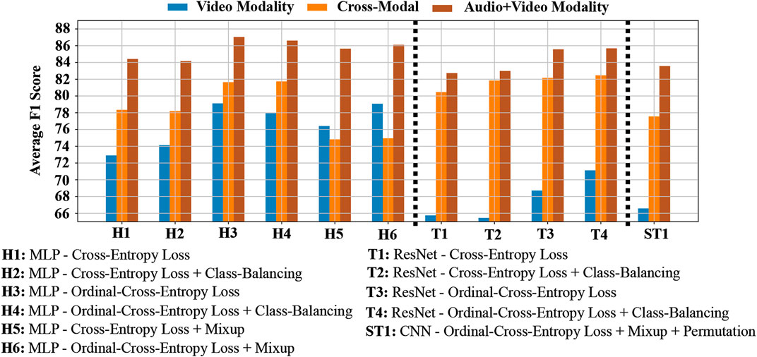
FIGURE 9. Weighted F1-score performance of the different Level B2 features in the Video, Cross-modal and Audio + Video modality settings.
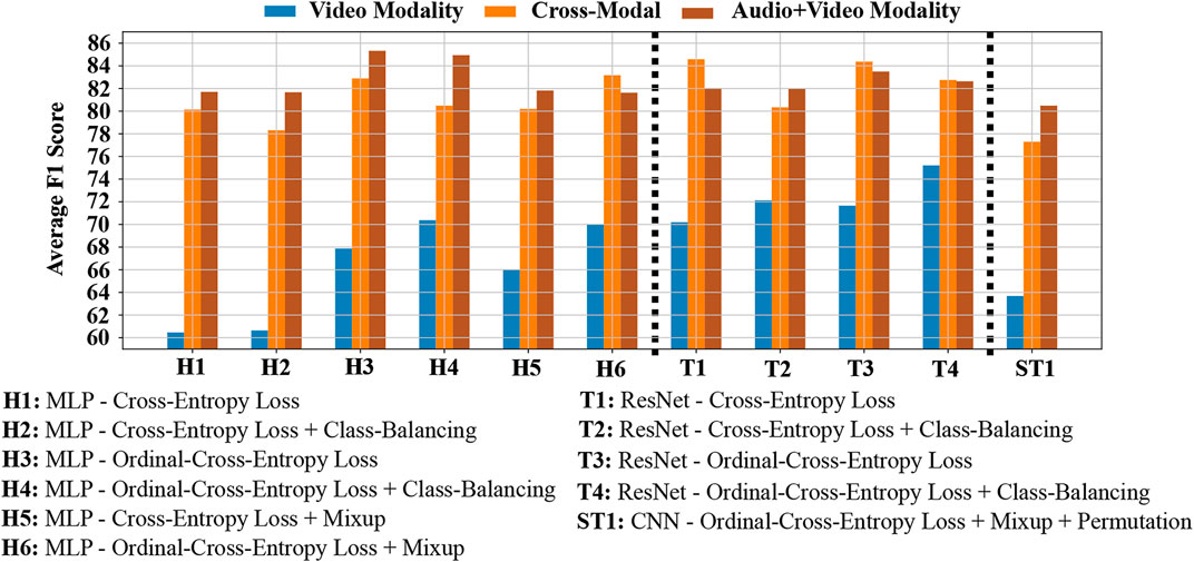
FIGURE 10. Weighted F1-score performance of the different Level C features in the Video, Cross-modal and Audio + Video modality settings.
This is an important finding as it implies that for the lower levels in CCM model (like B2, C), visual cues alone can help capture important details in the video recording. However, complex, higher level information like group collaboration requires both Audio and Video information for it to be accurately coded. We do not deny that Audio information is important even for the lower levels, but we believe that we can get away with a reasonably good deep-learning model in the situations where audio recording is not available. This is also similar to practical real-world setup. Teachers often have to assess non-verbal cues to determine the state of each student and the level of collaboration between members of the group.
5.4 Recommendation System
So far we discussed the collaboration assessment performance of the different feature representations under different modality settings. Based on the graphs and tables seen so far, one could be inclined to use either histogram or temporal representations for effectively estimating student collaboration quality. We have no reservations about this thought. In fact, we feel that if the purpose of the automated system is only to predict collaboration quality then the histogram or temporal representation should suffice. However, if one wants to develop an automated feedback or recommendation system, then spatio-temporal representations should be the way to go. Spatio-temporal representations along with the simple 2D CNN models proposed in this paper allow us to identify important temporal instances and isolate import student subsets at those instances. This level of detail is necessary in order to effectively provide recommendations.
The recommendation system proposed in this paper follows a stochastic-gradient-descent optimization framework. Stochastic-gradient-descent is the underlying mechanism on which all current state-of-the-art deep-learning systems are based on. Traditionally, the weights of the deep-learning model are optimized by minimizing a loss function. The loss function can be the cross-entropy or the ordinal-cross-entropy loss, as it is used to compute the error between the predicted and ground-truth labels. Next, back-propagation is used to calculate the gradient of the loss function with respect to each weight in the model. Finally, the gradient information is used by an optimization algorithm to update the model weights.
We use the process described above in a slightly different way for developing the recommendation system. Instead of optimizing the model’s weights, we now optimize the input spatio-temporal sample for which we want to generate recommendations. To do this we first use a pre-trained 2D CNN model that was trained using the spatio-temporal representations. The weights of the pre-trained model are frozen and not updated in the recommendation system. Next, we use the same loss function that was used to train the model, i.e., the ordinal-cross-entropy loss. However, a different loss function could also be used in this step. Next, we use back-propagation to calculate the gradient of the loss function with respect to each element in the spatio-temporal data sample. Finally, we use the gradient information to update important regions in the spatio-temporal sample that will help minimize the loss function error.
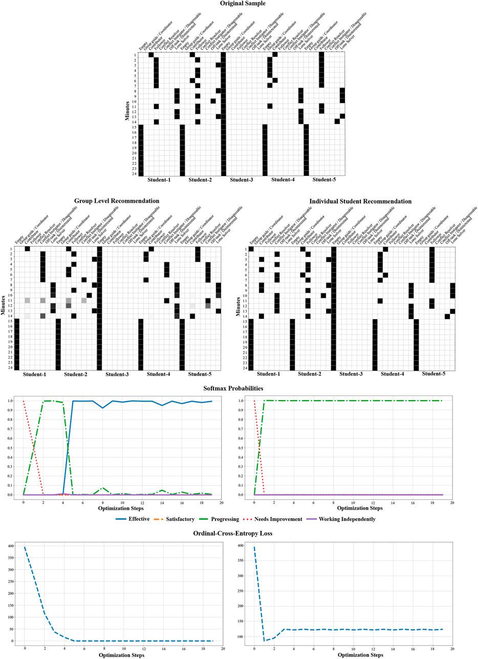
The final step described above can be done in many different ways. Using the gradient information we could update information of all the students in the spatio-temporal sample, which would result in a group level recommendation. We could also restrict the optimization process to only one student or a subset of students, which results in individual student level recommendations. Figure 11 shows an example of our recommendation system providing group level and individual student level recommendations for Level B2. In both cases the target label was set to Effective. The original sample only contains Level B2 information of four students (Student-3 is empty) and its collaboration quality was predicted as Needs Improvement. For group level recommendation, our recommendation system optimizes over the entire valid region of the sample (i.e., only for students present in the group and for the original task duration) till the generated sample is predicted as Effective. We observe that the softmax probabilities of Needs Improvement was initially high; followed by the Progressive code and finally settling at Effective. We also notice that the ordinal-cross-entropy loss becomes zero once the sample is predicted as Effective. Since the pre-trained model was trained using Mixup augmentation, our recommendation system tends to update the sample by following the ordered nature of the label space during the optimization process. During the optimization process the recommendation system in most cases is able to optimize and suggest a new role with high confidence or retains the same role at each time instance for each student. However, sometimes the system can get confused between multiple roles as illustrated at minutes 11 and 14 for student 1, minute 11 for student 2 and minute 12 for student 5 under the group level recommendation example in Figure 11. This implies that the system suggests a weighted combination of multiple roles in such cases. One can easily address such cases by simply doing a post-processing step and only consider the role that has the highest confidence.
In Figure 11 we also show an example of individual student recommendation. Here, we only optimize and provide recommendations for Student-1. The optimization space now is significantly less than the previous case. Due to this the recommendation system is only able to update the spatio-temporal sample that has a higher confidence in being Progressive. For the same reason the ordinal-cross-entropy loss function does not get minimized all the way to zero. This is similar to a realistic scenario, since it is very unlikely or rather very difficult to offer a recommendation to one student that will drastically improve the overall collaboration quality of the group.
In addition to providing positive feedback and recommendations, our system is also capable of showing scenarios of bad student roles that can further hamper the overall collaboration quality. For example, by simply setting the target label to Working Independently, our recommendation system can update the sample to show a scenario of either everyone or specific students in the group exhibiting poor individual roles. An important thing to note here is that the recommendations generated by our system is entirely dependent on how well the pre-trained classification model is trained. Biases learnt by the model can be reflected in the recommendations provided by the system. Also, the patterns for the recommendations generated are similar to the patterns observed in the co-occurrence matrices illustrated in Figure 4.
6 Conclusion
In this paper we proposed using simple 2D CNN models with spatio-temporal representations of individual student roles and behaviors, and compared their performance to temporal ResNet and MLP deep-learning architectures for student group collaboration assessment. Our objective was to develop more explainable systems that allow one to understand which instances in the input feature space and which subsets of students contributed the most towards the deep-learning model’s decision. We compared the performance of spatio-temporal representations against their histogram and temporal representation counterparts (Som et al., 2020; Som et al., 2021). While histogram and temporal representations alone can help achieve high classification performance, they do not offer the same key insights that we get using the spatio-temporal representations.
In our paper we also help bridge the performance gap between the Video and Audio + Video modalities by proposing the Cross-modal setting. In this setting we use feature representations from the Video modality and map it to labels collected in the Audio + Video modality. This setup can help reduce the cost, energy and time taken to collect, annotate and analyze audio recordings pertaining to student roles and behaviors. Through our empirical experiments we also found the importance of using both Audio and Video recordings to create more accurate overall student group collaboration annotations/codes. Group collaboration is a far more complicated process and might not be effectively captured with Video recordings alone, as suggested by the classification performance in the Video modality setting where both input features and target labels were obtained using only Video recordings.
Using the spatio-temporal representations and 2D CNN models we also proposed an automated recommendation system. This system is built on top of the 2D CNN model that was trained for assessing overall group collaboration quality. We considered both teachers and students as the target users when developing the system and demonstrated how it can be used for providing group level or individual student level recommendations of improved student roles. Teachers can first visualize the recommendations provided by the system and communicate it with the students or the students themselves can check the recommendations and approach the teacher for more insight.
6.1 Limitations and Future Work
The analysis and findings discussed in this paper can help guide and shape future work in this area. Having said that our approach of using 2D CNN models with spatio-temporal features can be further extended and improved in several ways. For starters, we can explore more complex and sophisticated deep-learning models to further push the performance of the spatio-temporal representations. The spatio-temporal representation design assumes that we have prior knowledge of the maximum task length. We can search for alternative representation designs that offer robustness to this requirement.
The proposed recommendation quantitatively behaves the way we expect it to. However, evaluating the quality of the recommendations is beyond the scope of this paper. In the future we plan to evaluate the recommendation quality by working closely with teachers. We also intend to check the usefulness of the recommendations by using surveys to ask students to rate the recommendations they received and whether it benefited them at different periods during the school year. For the recommendation system we can also search for more innovative ways to optimize the recommendations. We could use tools like LIME (Ribeiro et al., 2016) and SHAP (Lundberg and Lee, 2017) to aid in the recommendation process. These packages compute the importance of the different input features and help towards better model explainability and interpretability. Another possible research direction could be to use information from teachers or the student’s profile as prior information to better assist the recommendation process. We could also have teachers modify the recommendations provided by our system in an active learning setting which will help fine-tune the machine learning model and correct future recommendations. In this paper we only focused on mapping deep learning models from individual student roles and behaviors to overall group collaboration. In the future we intend on exploring other branches in the collaboration conceptual model, as described in Figure 1.
Data Availability Statement
The original contributions presented in the study are included in the article/supplementary files, further inquiries can be directed to the corresponding author.
Ethics Statement
The studies involving human participants were reviewed and approved by IRB training and approval was done. Written informed consent to participate in this study was provided by the participants’ legal guardian/next of kin.
Author Contributions
AS is a computer vision researcher and the machine learning lead for the project. He lead the development of the different machine learning models described in this paper. SK is a computer vision researcher. She was responsible for curating and processing the data for analysis and inference. BL-P is an education researcher. He lead the IRR analysis of the annotation data. SD is a computer vision researcher. She lead the data annotation and collection process. NA is a science education researcher and served as the PI for the project. She supervised the data collection, annotation and training processes. AT is a computer vision researcher and served as the Co-PI for the project. He supervised the machine learning and data analysis aspects of the project.
Funding
This work was supported in part by NSF grant number 2016849.
Conflict of Interest
The authors declare that the research was conducted in the absence of any commercial or financial relationships that could be construed as a potential conflict of interest.
Publisher’s Note
All claims expressed in this article are solely those of the authors and do not necessarily represent those of their affiliated organizations, or those of the publisher, the editors and the reviewers. Any product that may be evaluated in this article, or claim that may be made by its manufacturer, is not guaranteed or endorsed by the publisher.
References
Alexandron, G., Ruipérez-Valiente, J. A., and Pritchard, D. E. (2019). “Towards a General Purpose Anomaly Detection Method to Identify Cheaters in Massive Open Online Courses,” in Proceedings of the 12th International Conference on Educational Data Mining (EDM), Montreal, Canada, 480, 483.
Alozie, N., Dhamija, S., McBride, E., and Tamrakar, A. (2020a). “Automated Collaboration Assessment Using Behavioral Analytics,” in International Conference of the Learning Sciences (ICLS), Nashville, Tennessee (International Society of the Learning Sciences), 1071–1078. doi:10.22318/icls2020.1071
Alozie, N., McBride, E., and Dhamija, S. (2020b). American Educational Research Association (AERA) Annual Meeting. San Francisco, CA. Available at: http://tinyurl.com/sy3phcw.
Anaya, A. R., and Boticario, J. G. (2011). Application of Machine Learning Techniques to Analyse Student Interactions and Improve the Collaboration Process. Expert Syst. Appl. 38, 1171–1181. doi:10.1016/j.eswa.2010.05.010
Chollet, F. (2015). Keras. Available at: https://keras.io.
Daggett, W. R., and GendroO, D. S. (2010). Common Core State Standards Initiative. International center.
Davidson, N., and Major, C. H. (2014). Boundary Crossings: Cooperative Learning, Collaborative Learning, and Problem-Based Learning. J. Excell. Coll. Teach. 25, 7–55.
Genolini, C., and Falissard, B. (2011). Kml: A Package to Cluster Longitudinal Data. Comp. Methods Programs Biomed. 104, e112–e121. doi:10.1016/j.cmpb.2011.05.008
Guo, Z., and Barmaki, R. (2019). “Collaboration Analysis Using Object Detection,” in Proceedings of the 12th International Conference on Educational Data Mining, EDM 2019, Montréal, Canada, July 2-5, 2019 (International Educational Data Mining Society (IEDMS)).
Huang, K., Bryant, T., and Schneider, B. (2019). “Identifying Collaborative Learning States Using Unsupervised Machine Learning on Eye-Tracking, Physiological and Motion Sensor Data,” in Proceedings of the 12th International Conference on Educational Data Mining, EDM 2019, Montréal, Canada, July 2-5, 2019 (International Educational Data Mining Society).
Kang, J., An, D., Yan, L., and Liu, M. (2019). “Collaborative Problem-Solving Process in a Science Serious Game: Exploring Group Action Similarity Trajectory,” in Proceedings of the 12th International Conference on Educational Data Mining, EDM 2019, Montréal, Canada, July 2-5, 2019 (International Educational Data Mining Society).
Kingma, D. P., and Ba, J. (2014). Adam: A Method for Stochastic Optimization. arXiv preprint arXiv:1412.6980.
Krajcik, J. S., and Blumenfeld, P. C. (2006). “Project-based Learning,” in The Cambridge Handbook of the Learning Sciences. Editor R. Keith Sawyer (Cambridge University Press).
Loughry, M. L., Ohland, M. W., and DeWayne Moore, D. (2007). Development of a Theory-Based Assessment of Team Member Effectiveness. Educ. Psychol. Meas. 67, 505–524. doi:10.1177/0013164406292085
Lundberg, S., and Lee, S.-I. (2017). “A Unified Approach to Interpreting Model Predictions,” in Proceedings of the 31st International Conference on Neural Information Processing Systems, Long Beach, CA.
Reilly, J. M., and Schneider, B. (2019). “Predicting the Quality of Collaborative Problem Solving through Linguistic Analysis of Discourse,” in Proceedings of the 12th International Conference on Educational Data Mining, EDM 2019, Montréal, Canada, July 2-5, 2019 (International Educational Data Mining Society).
Ribeiro, M. T., Singh, S., and Guestrin, C. (2016). “Why Should I Trust You?” Explaining the Predictions of Any Classifier,” in Proceedings of the 22nd ACM SIGKDD international conference on knowledge discovery and data mining, San Francisco California USA, August 13-17, 2016 (Association for Computing Machinery), 1135–1144.
Selvaraju, R. R., Cogswell, M., Das, A., Vedantam, R., Parikh, D., and Batra, D. (2017). “Grad-cam: Visual Explanations from Deep Networks via Gradient-Based Localization,” in Proceedings of the IEEE international conference on computer vision, Venice, Italy, 22-29 Oct. 2017 (IEEE), 618–626. doi:10.1109/ICCV.2017.74
Smith-Jentsch, K. A., Cannon-Bowers, J. A., Tannenbaum, S. I., and Salas, E. (2008). Guided Team Self-Correction. Small Group Res. 39, 303–327. doi:10.1177/1046496408317794
Soller, A., Wiebe, J., and Lesgold, A. (2002). “A Machine Learning Approach to Assessing Knowledge Sharing during Collaborative Learning Activities,” in CSCL '02: Proceedings of the Conference on Computer Support for Collaborative Learning: Foundations for a CSCL Community, January 2002, 128–137. doi:10.3115/1658616.1658635
Som, A., Kim, S., Lopez-Prado, B., Dhamija, S., Alozie, N., and Tamrakar, A. (2020). “A Machine Learning Approach to Assess Student Group Collaboration Using Individual Level Behavioral Cues,” in European Conference on Computer Vision Workshops, Glasgow, UK, August 23–2 (Springer), 79–94. doi:10.1007/978-3-030-65414-6_8
Som, A., Kim, S., Lopez-Prado, B., Dhamija, S., Alozie, N., and Tamrakar, A. (2021). “Towards Explainable Student Group Collaboration Assessment Models Using Temporal Representations of Individual Student Roles,” in Educational Data Mining Conference, Paris, France, June 29-July 2, 2021.
Spikol, D., Ruffaldi, E., and Cukurova, M. (2017). Using Multimodal Learning Analytics to Identify Aspects of Collaboration in Project-Based Learning. Philadelphia, PA: International Society of the Learning Sciences.
States, N. L. (2013). Next Generation Science Standards: For States, by States. Washington, DC: The National Academies Press.
Taggar, S., and Brown, T. C. (2001). Problem-Solving Team Behaviors. Small Group Res. 32, 698–726. doi:10.1177/104649640103200602
Talavera, L., and Gaudioso, E. (2004). “Mining Student Data to Characterize Similar Behavior Groups in Unstructured Collaboration Spaces,” in Workshop on artificial intelligence in CSCL. 16th European conference on artificial intelligence (Citeseer), 17–23.
Thulasidasan, S., Chennupati, G., Bilmes, J. A., Bhattacharya, T., and Michalak, S. (2019). “On Mixup Training: Improved Calibration and Predictive Uncertainty for Deep Neural Networks,” in Advances in Neural Information Processing Systems, 13888–13899. doi:10.2172/1525811
Vrzakova, H., Amon, M. J., Stewart, A., Duran, N. D., and D’Mello, S. K. (2020). “Focused or Stuck Together: Multimodal Patterns Reveal Triads’ Performance in Collaborative Problem Solving,” in Proceedings of the Tenth International Conference on Learning Analytics & Knowledge, 295–304.
Wang, Z., Yan, W., and Oates, T. (2017). “Time Series Classification from Scratch with Deep Neural Networks: A strong Baseline,” in 2017 International joint conference on neural networks (IJCNN) (IEEE), 1578–1585. doi:10.1109/ijcnn.2017.7966039
Wittenburg, P., Brugman, H., Russel, A., Klassmann, A., and Sloetjes, H. (2006). “Elan: A Professional Framework for Multimodality Research,” in 5th International Conference on Language Resources and Evaluation (LREC 2006), Genoa, Italy (European Language Resources Association (ELRA)), 1556–1559.
Keywords: k-12, education, collaboration assessment, feedback system, deep learning, machine learning
Citation: Som A, Kim S, Lopez-Prado B, Dhamija S, Alozie N and Tamrakar A (2021) Automated Student Group Collaboration Assessment and Recommendation System Using Individual Role and Behavioral Cues. Front. Comput. Sci. 3:728801. doi: 10.3389/fcomp.2021.728801
Received: 22 June 2021; Accepted: 24 August 2021;
Published: 14 October 2021.
Edited by:
Ronald Böck, Otto von Guericke University Magdeburg, GermanyReviewed by:
Dulce Fernandes Mota, Instituto Superior de Engenharia do Porto (ISEP), PortugalMaria Koutsombogera, Trinity College Dublin, Ireland
Copyright © 2021 Som, Kim, Lopez-Prado, Dhamija, Alozie and Tamrakar. This is an open-access article distributed under the terms of the Creative Commons Attribution License (CC BY). The use, distribution or reproduction in other forums is permitted, provided the original author(s) and the copyright owner(s) are credited and that the original publication in this journal is cited, in accordance with accepted academic practice. No use, distribution or reproduction is permitted which does not comply with these terms.
*Correspondence: Anirudh Som , YW5pcnVkaC5zb21Ac3JpLmNvbQ==
 Anirudh Som
 Sujeong Kim1
