Quantum-Inspired Uncertainty Quantification

Reasonable quantification of uncertainty is a major issue of cognitive infocommunications, and logic is a backbone for successful communication. Here, an axiomatic approach to quantum logic, which highlights similarity to and differences to classical logic, is presented. The axiomatic method ensures that applications are not restricted to quantum physics. Based on this, algorithms are developed that assign to an incoming signal a similarity measure to a pattern generated by a set of training signals.

1 Introduction

Reasonable quantification of uncertainty is a major issue of cognitive infocommunications, and logic is a backbone for successful communication. The motivation for writing this article came from some experience with fuzzy logic in industrial context, and from the observation that quantum logic appears to be superior to other “fuzzy” approaches; see, for instance, Schmitt and Nurnberger (2007).

This paper describes a mathematically rigorous pathway from classical logic to mathematical models that enable a quantification of uncertainty. Such models had been developed and studied especially in the context of quantum physics, where a link to probability is given by Born’s postulate. Hence, both classical logic with and, or, and negation, and the mathematics of quantum mechanics are in the focus of this article.

An axiomatic approach to quantum logic has two advantages: It highlights the relation between classical logic and quantum logic, and it shows that application of quantum logic is not restricted to quantum physics. The result is that a classical system of propositions can be represented as Boolean lattice, and a quantum system of propositions is represented by an atomistic orthomodular lattice. Quantum logic contains several variants of classical logic, as an atomistic orthomodular lattice has several Boolean sublattices.

In a human–machine communication process, the communicative acts often can be described by real functions defined on an interval [a, b]. Morover, a proposition often can be represented by a finitely generated subspace of L² ([a, b]). The final section of this article describes how to use Gram-Schmidt processes for representing logical operations by dealing with generating families and constructing orthonormal families which span linear subspaces corresponding to logical expressions.

2 Quantum Logic: An Axiomatic Approach

In a historic perspective, quantum logic originated in an article by Birkhoff and von Neumann (1936) entitled The Logic of Quantum Mechanics, which appeared in the Annals of Mathematics. The authors discover logical structures in quantum mechanics and come to the conclusion that

“one can reasonably expect to find a calculus of propositions which is formally indistinguishable from the calculus of linear subspaces with respect to set products, linear sums, and orthogonal complements—and resembles the usual calculus of propositions with respect to and, or, and not.”

It was known at that time that the “usual calculus of propositions” means that the set of propositions carries the algebraic structure Boolean lattice with two binary operations called conjunction (logical and, ∧) and adjunction (logical or, ∨), and a unary operation called negation (logical not, ¬). Let us now go to the next major step towards the mathematics of quantum logic.

2.1 Piron’s Axiomatique Quantique

According to Piron (1964), the system $\mathbb{L}$ of propositions fulfills the following axioms.

Axiom O: Implication is a partial order on $\mathbb{L}$, denoted by ⩽.

A requirement of this axiom is that implication is transitive, which reflects the classical Barbara syllogism.

The next axiom uses the notion indexed family of propositions, which is a map $J\to \mathbb{L}$ from an arbitrarily given index set J to the system $\mathbb{L}$. This map associates to each j ∈ J a proposition $a_j\in \mathbb{L}$.

Axiom T: For any family of propositions {a_j: j ∈ J}, there is an infimum w.r.t. the partial order ⩽, i.e., a proposition $u\in \mathbb{L}$ that fulfills for any $x\in \mathbb{L}$ the equivalence.

$x⩽a_j\text{\hspace{0.17em}for\hspace{0.17em}any\hspace{0.17em}}j\in J\iff x⩽u.$

This proposition is denoted by u = inf{a_j: j ∈ J} (Piron uses the notation ⋂_Ja_j).

This axiom requires that the logical conjunction of an arbitrary set of propositions is again a proposition.

The following lattice theoretic notation is used here: $\varphi ≔\inf \mathbb{L}$ is the bottom of the lattice, and for $a,b\in \mathbb{L}$, define their meet by a ⊓ b≔ inf{a, b} (Piron uses the curved symbol a ∩ b). The following axioms are given in Piron (1964) formally weaker than the formulations given here, but it is possible to derive the formulae given here from Piron’s statements.

Axiom C: There is on $\mathbb{L}$ an orthocomplementation a↦a′, which is involutive, a^″ = a, subject to the law of noncontradiction a ⊓ a′ = ϕ, and it admits the modus tollens a⩽b ⇔ b′⩽a′.

Axiom C means that orthocomplementation is a mathematical model for logical negation.

Based on orthocomplement, the join of two propositions $a,b\in \mathbb{L}$ is defined by de Morgan’s law a ⊔ b≔(a′ ⊓ b′)′ (again, Piron prefers the curved symbol a ∪ b—which is misleading here, as it turns out that a ⊔ b is not to be confused with a set-theoretic union).

The three axioms O, T and C ensure that the system of propositions $\mathbb{L}$ with meet and join and orthocomplementation as above carries the algebraic structure orthocomplemented lattice. This is the algebraic structure that is common to both classical logic and quantum logic. Based on investigations in Boole (1847), classical mathematical logic focused its attention to Boolean lattices. From an axiomatic point of view, a Boolean lattice is an orthocomplemented lattice that fulfills a law of distributivity. In quantum logic, distributivity is replaced by more general algebraic properties. It remains crucial that certain sublattices of $\mathbb{L}$ are Boolean, e.g., see the following axiom.

Axiom P: If a⩽b, then the sublattice generated by a and b is Boolean.

This axiom marks the difference between classical logic and quantum logic. It formulates that physical measurements that correspond to propositions satisfying the relation a⩽b are compatible.

In lattice theory, an element $a\in \mathbb{L}$ with a ≠ ϕ is called an atom, if ϕ⩽u⩽a implies u ∈ {ϕ, a}. Piron writes point instead of atom and uses capital letters P, Q, … for denoting points.

Axiom A: 1) For any $a\in \mathbb{L}$ with a ≠ ϕ, there is a point P with ϕ⩽P⩽a.

2) If Q is point and a⩽x⩽a ⊔ Q, then x ∈ {a, a ⊔ Q}.

Axiom A requires that the set $\mathbb{L}$ of propositions contains sufficiently many atomic propositions.

Calling the join P ⊔ Q of two points P and Q a straight line, the points and straight lines make up an incidence geometry; see, for instance, Beutelspacher and Rosenbaum (2004). In addition, Piron (1964) proves that, in this structure, the following Veblen-Young-Axiom holds:

If A, B, C are points not all on the same line, and D and E (D ≠ E) are points such that B, C, D are on a line and C, A, E are on a line, there is a point F such that A, B, F are on a line and also D, E, F are on a line. (Veblen and Young, 1918, p. 2).

This connects quantum logic to projective geometry—a fact that will turn out to be crucial for our application.

2.2 Piron’s Theorem

The main result in Piron (1964) is that, provided the system $\mathbb{L}$ of propositions is rich enough to include at least four propositions with the property that none of them implies the join of the other three, then Axioms O, T, C, P, and A imply that the propositions in $\mathbb{L}$ are in one–one correspondence with the closed linear subspaces of a Hermitian vector space.

More precisely, he proves that there is a division ring $\mathbb{K}$ and a left $\mathbb{K}$-vector space $\mathbb{V}$ with a non-degenerate Hermitian form ⟨x, y⟩. This Hermitian form allows to define the orthocomplement of any set $S\subseteq \mathbb{V}$ of vectors by $S^{\perp }≔\{v\in \mathbb{V}:⟨v,s⟩=0\text{\hspace{0.17em}for\hspace{0.17em}any\hspace{0.17em}}s\in S\}$. In this setting, a subspace $S\subseteq \mathbb{L}$ is said to be closed, if S = S^⊥⊥. Moreover, it is implied that the Hermitian form is orthomodular, which means that any closed subspace $S\subseteq \mathbb{V}$ fulfills the equation $S+S^{\perp }=\mathbb{V}$.

In this setting, if a proposition a corresponds to closed linear subspace $\tilde{a}\subseteq \mathbb{V}$, then the negation a′ corresponds to the orthocomplement ${\tilde{a}}^{\perp }$. Similarly, if two propositions a₁ and a₂ correspond to closed linear subspaces ${\tilde{a}}_1\subseteq \mathbb{V}$ and ${\tilde{a}}_2\subseteq \mathbb{V}$, their meet a ⊓ b corresponds to the intersection ${\tilde{a}}_1\cap {\tilde{a}}_2$, and their join a₁ ⊔ a₂ corresponds to the closure of the vector sum ${\tilde{a}}_1+{\tilde{a}}_2=\{x+y:x\in {\tilde{a}}_1,y\in {\tilde{a}}_2\}\subseteq \mathbb{V}$. Based on these correspondences, the orthomodular law for the Hermitian form is equivalent to the classical law of excluded middle for the corresponding propositions.

2.3 Solèr’s Condition and Hilbert Space

Given a division ring $\mathbb{K}$ and a left $\mathbb{K}$-vector space $\mathbb{V}$ with a non-degenerate orthomodular Hermitian form on $\mathbb{V}$, a family {v_j: j ∈ J} is called orthonormal, if

$⟨v_i,v_j⟩=\left\{\begin{array}{cc}1\hfill & \text{if\hspace{0.17em}}i=j,\hfill \\ 0\hfill & \text{if\hspace{0.17em}}i\ne j.\hfill \end{array}\right.$

Solèr’s theorem is based on a classical theorem of Frobenius, which states that there are exactly three different real division algebras: the real numbers $\mathbb{R}$, the complex numbers $\mathbb{C}$, and the Hamiltonian quaternions $\mathbb{H}$. Now, the key result in Solèr (1994) is: If there is an infinite orthonormal family in $\mathbb{L}$, then $\mathbb{K}$ is a real division algebra and $\mathbb{V}$ is a classical Hilbert space.

It is known from Piron’s theorem that any proposition corresponds to a closed subspace of $\mathbb{V}$. Physicists also call a proposition an event, emphasizing the fact that measuring a property projects the system onto a state belonging to the result of measurement. In a Hilbert space model used in quantum physics, a proposition, or an event, is given either by a closed subspace, or by an orthogonal projector, which is a self-adjoint idempotent linear operator. Moreover, if a quantum system is described by a unit vector in $\mathbb{V}$, then, according to Born’s postulate, the probability that a measurement produces the result that the system makes a proposition a true is given by the square length of the orthogonal projection of the unit vector to the closed linear subspace corresponding to a. The mathematics starting at logic and leading to the computation of probabilities is outlined in Figure 1.

FIGURE 1

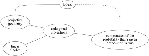
FIGURE 1. The relations between logic, projective geometry, linear algebra, orthogonal projections, and the computation of probabilities.

3 Quantification of Signal Similarity

3.1 Modeling With Hilbert Space

For modeling human–machine communicative situations, we restrict attention to real Hilbert spaces. In this case, the non-degenerate orthomodular Hermitian form reduces to a real scalar product. Specifically, we consider a fixed real interval [a, b] and the Hilbert space $\mathbb{V}≔L^2([a,b])$ of square-integrable functions $x,y:[a,b]\to \mathbb{R}$ with their scalar product given by integration

$⟨x|y⟩≔{\int }_a^{b}x(t)y(t)dt.(1)$

Here, we use the intuitive ket-bra-notation introduced by Dirac (1939): An element of the Hilbert space is a ket vector $\left|y\right.⟩$; for writing an element $\left|x\right.⟩$ at the first place of a scalar product, it is necessary to take its adjoint, which is a bra vector $\left.⟨x\right|={\left|x\right.⟩}^{†}$; combining a bra with a ket vector gives a braket $⟨x|y⟩$, which is just the scalar product of the two elements. One advantage of this notation is a nice formula for orthogonal projectors: Given a closed subspace a spanned by an orthonormal family {v_j: j ∈ J}, the orthogonal projector $P_a:\mathbb{V}\to a$ is given by

$P_a=\sum _{j\in J}|v_j\rangle \langle v_j|\text{\hspace{0.17em}with\hspace{0.17em}\hspace{0.17em}}{P}_a|x\rangle =\sum _{j\in J}|v_j\rangle \langle v_j|x\rangle .$

Note that in Dirac’s ket and bra notation, it appears more natural to consider the Hilbert space as a right vector space, i.e., the scalars come from the right-hand side. For calculating the projection probability p_a(x) of a ket vector $\left|x\right.⟩$ onto a, first ensure that $⟨x|x⟩=1$, and then use Born’s postulate to compute

$p_a(x)={\left(P_a|x\rangle \right)}^{†}{P}_a|x\rangle =\langle x|P_a^{†}{P}_a|x\rangle =\langle x|P_a|x\rangle =\sum _{j\in J}\langle x|v_j\rangle \langle v_j|x\rangle .$

In this calculation, it is used that an orthogonal projector is self-adjoint and idempotent.

Note that in Eq. 1, a certain “modeling freedom” is used. Here, it would be possible to introduce an appropriate weighting function, but this would only be reasonable if a good substantiation were provided.

3.2 Algorithms Used for Calculation

First assume for simplicity that all signals are sampled on an interval [a, b] with the same sampling rate. This means that there are time points t₀ = a < t₁ < … < t_n = b such that, given a signal $x:[a,b]\to \mathbb{R}$, the numbers x (t_j) for j ∈ {0, … , n} are recorded. In this setting, a scalar product is approximated using the trapezoidal rule

${\int }_a^{b}x(t)y(t)dt\approx \frac{1}{2}\sum _{j=0}^{n-1}x(t_j)y(t_j)(t_{j+1}-t_j)+\frac{1}{2}\sum _{j=1}^{n}x(t_j)y(t_j)(t_j-t_{j-1}).$

Next, assume that training signals x₁, … , x_k are given, and that the question is whether or not an incoming signal x belongs to the pattern defined by the training signals. Or, more precisely, what is the probability p(x) that x belongs to the trained pattern? For answering this question, I propose the following steps:

1) Employ a Gram-Schmidt process for constructing an orthonormal base |v₁⟩, …, |v_ℓ⟩ for the subspace generated by |x₁⟩, …, |x_k⟩—note that, as the generating set is finite, this subspace is closed, and that its dimension is ℓ⩽k.

2) Normalize the incoming signal by setting $\left|\widehat{x}\right.⟩≔\frac{\left|x\right.⟩}{\sqrt{⟨x|x⟩}}$.

3) Evaluate the formula $p(x)={\sum }_{j=1}^{\ell }⟨\widehat{x}|v_j⟩⟨v_j|\widehat{x}⟩$.

A noteworthy special case is when just one training signal x₁ is given. Then,

$p(x)=\frac{{⟨x_1|x⟩}^2}{⟨x_1|x_1⟩⟨x|x⟩}.(2)$

3.3 Application to Logic

By Piron’s theorem, a logical proposition does not correspond to training signals, but rather to the subspace generated by them. The atoms of the lattice of propositions are the one-dimensional subspaces given $\left|x\right.⟩\mathbb{R}$, where x runs through the signals ≠ 0. We learn from projective geometry that a signal alone does not have a logical meaning, only the subspace $\left|x\right.⟩\mathbb{R}$ corresponds to a proposition. It is hard to imagine how to derive Eq. 2 without reference to quantum logic—that is what I mean with “quantum inspired”.

What about representing logical operations and, or, and negation? For a concise notation, assume that two propositions a and b correspond to two sets of training signals spanning closed subspaces $\tilde{a}=span(|x_1\rangle ,\dots ,|x_k\rangle )$ and $\tilde{b}=span(|y_1\rangle ,\dots ,|y_{\ell }\rangle )$.

1) Logical “or”: Running a Gram-Schmidt process on the sequence

$|x_1\rangle ,\dots ,|x_k\rangle ,|y_1\rangle ,\dots ,|y_{\ell }\rangle (3)$

leads to an orthonormal family generating the closed linear subspace $\tilde{a}+\tilde{b}$, which corresponds to the adjunction a ⊔ b in propositional calculus.

2) Relative negation: Here, the aim is to construct an orthonormal family generating the subspace

$\left(\tilde{a}+\tilde{b}\right)\cap {\tilde{a}}^{\perp }$

which corresponds to the proposition (a ⊔ b) ⊓ a′. To this end, run Gram-Schmidt on the sequence 3, and remove the first part that belongs to $\tilde{a}$.

3) Logical “and”: Apply de Morgan’s law to relative orthocomplements in $\tilde{a}+\tilde{b}$,

$\tilde{a}\cap \tilde{b}={\left({\tilde{a}}^{\perp }+{\tilde{b}}^{\perp }\right)}^{\perp }=\left(\tilde{a}+\tilde{b}\right)\cap {\left(\left(\left(\tilde{a}+\tilde{b}\right)\cap {\tilde{a}}^{\perp }\right)+\left(\left(\tilde{a}+\tilde{b}\right)\cap {\tilde{b}}^{\perp }\right)\right)}^{\perp }.(4)$

This reduces the logical “and” to logical “or” and relative negation. Along these lines, algorithms described above can be combined to construct an orthonormal base for the intersection of finitely generated subspaces.

4 Application to Signal Comparison

Quantum-inspired uncertainty quantification can be applied to signal comparison tasks. The procedure is as follows.

1) Ensure that all training signals have equal length. This can be done by cutting appropriately and/or by using linear transformations. The result should be a set of training signals x₁, … , x_k, which are defined on the same interval.

2) For handling the problem of possible different sampling rates, collect all sampling points and fill the missing data by linear interpolation. This is reasonable as we are only interested in the calculation of scalar products.

3) For an incoming signal, use cutting and/or rescaling to ensure that it is defined on the same interval as the training data.

4) Compute the projection probability p(x) of the incoming signal x to these training patterns using the procedure described in section 3.2.

Then, p(x) provides a measure of similarity between an incoming signal and the set of training signals.

Data Availability Statement

The original contributions presented in the study are included in the article/Supplementary Material. Further inquiries can be directed to the corresponding author.

Author Contributions

The author confirms being the sole contributor of this work and has approved it for publication.

Conflict of Interest

The author declares that the research was conducted in the absence of any commercial or financial relationships that could be construed as a potential conflict of interest.

Publisher’s Note

All claims expressed in this article are solely those of the authors and do not necessarily represent those of their affiliated organizations, or those of the publisher, the editors, and the reviewers. Any product that may be evaluated in this article, or claim that may be made by its manufacturer, is not guaranteed or endorsed by the publisher.

Acknowledgments

The idea to this logically founded quantification of uncertainty arose slowly during a long-term collaboration with Matthias Wolff and Ingo Schmitt, BTU Cottbus-Senftenberg. I am grateful to the Katholische Universität Eichstätt-Ingolstadt, where I hold a part-time teaching position, for supporting this work in many respects, including financially.

References

Beutelspacher, A., and Rosenbaum, U. (2004). Projektive Geometrie : von den Grundlagen bis zu den Anwendungen (Wiesbaden: Vieweg). edn, 2.

Google Scholar

Birkhoff, G., and Neumann, J. V. (1936). The Logic of Quantum Mechanics. Ann. Mathematics 37, 823–843. doi:10.2307/1968621

CrossRef Full Text | Google Scholar

Boole, G. (1847). The Mathematical Analysis of Logic : Being an Essay towards a Calculus of Deductive Reasoning. Cambridge: Macmillan.

Google Scholar

Dirac, P. A. M. (1939). A New Notation for Quantum Mechanics. Math. Proc. Camb. Phil. Soc. 35, 416–418. doi:10.1017/s0305004100021162

CrossRef Full Text | Google Scholar

Piron, C. (1964). Axiomatique Quantique. Helvetica Physica Acta, 439–468.

Google Scholar

Schmitt, I., and Nurnberger, A. (2007). “Image Database Search Using Fuzzy and Quantum Logic,” in 2007 IEEE International Fuzzy Systems Conference, London, UK, 23-26 July 2007, 1–6. doi:10.1109/FUZZY.2007.4295682

CrossRef Full Text | Google Scholar

Solèr, M. P. (1994). Charakterisierung von Hilberträumen als spezielle orthomodulare Räume. Dissertation Universität Zürich, 22 Seiten.

Google Scholar

Veblen, O., and Young, J. W. (1918). Projective Geometry/2. Boston.

Google Scholar