Analysis and Classification of Word Co-Occurrence Networks From Alzheimer’s Patients and Controls

In this paper we construct word co-occurrence networks from transcript data of controls and patients with potential Alzheimer’s disease using the ADReSS challenge dataset of spontaneous speech. We examine measures of the structure of these networks for significant differences, finding that networks from Alzheimer’s patients have a lower heterogeneity and centralization, but a higher edge density. We then use these measures, a network embedding method and some measures from the word frequency distribution to classify the transcripts into control or Alzheimer’s, and to estimate the cognitive test score of a participant based on the transcript. We find it is possible to distinguish between the AD and control networks on structure alone, achieving 66.7% accuracy on the test set, and to predict cognitive scores with a root mean squared error of 5.675. Using the network measures is more successful than using the network embedding method. However, if the networks are shuffled we find relatively few of the measures are different, indicating that word frequency drives many of the network properties. This observation is borne out by the classification experiments, where word frequency measures perform similarly to the network measures.

1 Introduction

As populations continue to age, the development of automated methods to help reduce the amount of in person care required is becoming an important research topic. Dementia is a particular issue, where the cognitive function of a person declines as they age, with symptoms including memory loss, motor problems, deterioration of visuospatial function, language impairment and emotional distress. These issues tend to reduce the ability of a person to care for themselves, placing an added burden on their carers and/or relatives. Early diagnosis of dementia is desirable as it is amenable to treatment, and this can help the patient live a longer, more independent life. Dementia shows various linguistic effects, with patients tending to produce sentences with less information, less syntactic complexity (Pakhomov et al., 2011), fewer unique words and more meaningless sentences (Fraser et al., 2016). These effects can be used for non-invasive diagnosis and analysis of dementia, and so in this paper we look at using text classification methods to this end.

The common approach in text classification is to use a bag of words model. This assumes that word order does not matter, and either counts the number of occurrences of each word in a document, or uses some information based measures such as term-frequency inverse document frequency (TF-IDF). Various authors have taken this approach, and demonstrated good results on classifying participants as AD or controls (Orimaye et al., 2017; Wankerl et al., 2017). However, word order does in fact matter, and we can try to capture this using graph based methods. The approach used here is to construct a graph where the words in the document are nodes, and if two words co-occur within a certain window (a set of words occurring around a given word) an edge is drawn between them. Furthermore, these co-occurrence networks are an approximation of syntactic networks, as most syntactic relationships occur between words that are close together (Cancho and Solé, 2001). Various syntactic measures have been previously used to distinguish between AD patients and controls (Pakhomov et al., 2011; Fraser et al., 2016), and we hypothesize that these co-occurrence networks can capture these syntactic relations without the use of a syntactic parser.

Therefore, in this paper we investigate the properties of word co-occurrence networks using a variety of co-occurrence windows from transcripts of controls and patients diagnosed with potential Alzheimer’s disease (AD) on a picture description task. We analyze these networks for potential differences between the controls and AD patients using various network measures, and then look at classifying the networks using a set of network measures, a graph embedding method and a baseline method using word frequency statistics. Each transcript is also annotated with the mini-mental state examination (MMSE) result. This is a test of cognitive function, and can be used to help diagnose dementia. The test scores ranges from 0–30, and a score below 24 is usually taken to indicate cognitive impairment. We are also interested in predicting the value of the MMSE score from a transcript by using this co-occurrence network model and the graph measures/network embedding method. To the best of our knowledge, such an approach has not been taken before. We use the terms graph and network interchangeably in this paper, and we emphasize these networks we refer to are different to neural networks.

2 Related Work

The structure of word co-occurrence networks has been studied by many authors, along with which parameters can be used for classification. For instance Liu and Cong (2013) study the use of various network measures for distinguishing between the same text written in a set of different languages. Focusing mostly on Slavic languages (although they do also use English) they use hierarchical clustering to show which languages are more similar. By trying many different combinations of the network measures, they discover that it is possible to show the Slavic languages are more similar to each other than they are to English or Chinese, and inside the Slavic group the languages that are generally regarded as more similar (e.g. Belorussian and Russian) are more closely clustered than less similar languages (e.g. Russian and Slovakian). Other authors have applied similar methods for author attribution (Antiqueira et al., 2007; Mehri et al., 2012; Akimushkin et al., 2017), distinguishing between automatically generated and human written text (Amancio et al., 2008; Amancio, 2015) and for keyphrase extraction (Mihalcea and Tarau, 2004; Bougouin et al., 2013; Florescu and Caragea, 2017). A detailed review of the literature so far on the construction and applications of word co-occurrence networks is provided by Cong and Liu (2014).

Graphs can also be used to augment n-gram classification. For instance, we can gain the centrality of a term from a graph, which can then be used as input into a text classification algorithm (Hassan et al., 2007), and this has been shown to improve classification accuracy compared to just using n-grams. Alternatively we can use the structure of the graph as input into the classification algorithm. This has the advantage of ensuring that new documents can have unknown words, which is advantageous if the system must be deployed for a period of time, as it is unlikely that every word that could ever be encountered is present in the training set. Rousseau et al. (2015) use the subgraph mining method gSpan (Yan and Han, 2002) to mine frequent subgraphs from a set of graphs extracted from text documents. The presence of these subgraphs is then used as input into the classification method. The disadvantage of this method is that it is computationally expensive to mine for all possible subgraphs of non-trivial size.

A similar approach to the one we take in this paper is proposed by Santos et al. (2017). In their paper the authors apply a word co-occurrence network model to the DementiaBank and a Portuguese dataset. However, unlike us they enrich their model using word embeddings to produce weighted edges between words that do not co-occur. They calculate node level statistics for each graph and use this as input into a classification procedure. With their enriched networks they achieve an increase in classification accuracy, achieving 62% on the DementiaBank dataset.

There have been many more approaches taken to identify Alzheimer’s using machine learning techniques and linguistic features. One of the first examples in the literature is the analysis of the books of an author who was diagnosed with Alzheimer’s by Garrard et al. (2005). A combination of lexical, syntactic and vocabulary based features is used to compare the books. This is further extended by Pakhomov et al. (2011). Using the Stanford parser, the authors take three measures of syntactic complexity, Yngve depth, Frazier depth and the length between grammatical dependencies. There is a clear decline over time in the syntactic complexity of the authors writing, particularly with the books at the end of her career.

Many authors have used the DementiaBank corpus for their studies. For instance, Fraser et al. (2016) apply machine learning methods to the DementiaBank corpus, using both transcripts and speech data. Firstly they used logistic regression to evaluate the contribute of each feature to successful classification of a participant as having Alzheimer’s or being a control. Ranking the features using Pearson correlation, they firstly investigate how including more features affects the classification accuracy. The maximum classification accuracy is achieved when the 35 most correlated features are used (at 81.92%), and beyond this it tends to remain roughly constant until 50 features are reached (dropping slightly to 78.72%, after which the classification accuracy decreases significantly. Of relevance to this paper, they find that AD patients produce more pronouns, fewer nouns, have a smaller vocabulary and repeat themselves more. Interestingly though, measures such as the depth of the parse tree do not seem significantly correlated with an AD diagnosis.

Orimaye et al. (2017) further explore which features can be used to distinguish between AD and controls from transcripts. A combination of n-grams, lexical and syntactic features to this end. Since this is a large feature set, they perform some univariate screening using t-tests to remove variables which have little ability to distinguish between classes. Of particular interest to us, they find that the number of repetitions, reduced sentences, predicates and mean length of utterances are different between the classes, but that many other syntactic measures, such as the dependency distance, are not. They then select the top 1,000 features for input into the SVM classifier. Comparing the syntactic and lexical features only, to the n-gram only, to the combination of the two, they find that the combination performs the best, with an AUC of 0.93, compared to 0.80 for the lexical-syntactic features and 0.91 for the n-gram features.

Authors have also disregarded syntactic features and used only n-grams for classification. For instance, Garrard et al. (2014) use n-grams to distinguish between AD patients and controls on a picture description task. They find that the transcripts from the controls contain more content words (e.g. picnic, blanket) while the AD patients tend to produce more generic terms (e.g. something, thing). They use only a small subset of the total word set to classify, as there are a large number of possible n-grams. This indicates that a small number of features can be used to distinguish between AD patients and controls.

Larger n-grams can also be used. Orimaye et al. (2018) use a deep neural network and large n-grams $\left(n>3\right)$ to classify the participants into control or AD. Since the occurrence matrix of these n-grams will be very sparse, they firstly reduce the dimensionality using SVD (selecting 19 features in the end), before inputting this smaller matrix into the neural network. Experimenting with a variety of n-gram sizes, they find using 4 g achieves the lowest error (11.1%) on the test set in their deep neural networks. It is also possible to use the distribution of n-grams to differentiate between AD and controls. Wankerl et al. (2017) create probability distributions of the trigrams in transcripts from the cookie detection task from DementiaBank. The perplexity of a new sample is used to classify it as AD or control.

While transcripts are convenient to analyze, transcription can be challenging, either noisy if done automatically or slow and expensive if done by humans. Using purely audio is attractive if we wish to apply these methods on non curated datasets. Haider et al. (2019) study the same corpus, but instead focus their efforts on purely acoustic features. Here they use a fusion of acoustic feature sets (namely emobase, ComParE, eGeMaps and MRCG) on the DementiaBank dataset, achieving a maximum accuracy of 78.8%. A challenge with many of these approaches is that they are dependent on language and context. To solve these issues, Luz et al. (2018) instead propose to extract vocalization graphs from patient dialogue. Using features from these vocalization graphs, they achieve a classification accuracy of 86.5%, though on a different dataset.

Aside from speech data, other approaches have included the use of smart home data (Alberdi et al., 2018). This particular example involves using activity recognition to establish routines, and then these routines can be compared between healthy participants and those with AD. If the reader is curious for more details, comprehensive reviews on the topic of Alzheimer’s detection are provided by de la Fuente Garcia et al. (2020) and Slegers et al. (2018).

3 Software and Data

Our dataset is made up of transcripts from the DementiaBank corpus. The DementiaBank corpus is a set of recordings of cognitive tests, which forms part of the larger TalkBank project (MacWhinney, 2019). The subset of DementiaBank used in this study encompasses recordings and their corresponding transcriptions, where patients with Alzheimer’s and controls describe a picture known as the “Cookie Theft” scene, taken from the Boston Diagnostic Aphasia Examination (Becker et al. (1994)). This dataset is known as the Pitt corpus. Participants were required to:

• be above 44 years of age,

• have at least 7 years of education,

• have no history of nervous system disorders,

• not be taking neuroleptic medication,

• have an MMSE score of above 10.

• be able to give informed consent, and

• have a caregiver or relative to act as an informant if they had dementia.

To avoid possible biases due to age and gender which might have affected some of the above mentioned machine learning studies (de la Fuente Garcia et al., 2020), we use the ADReSS challenge dataset (Luz et al., 2020). The age and gender distributions of participants in DementiaBank’s Pitt Corpus tend to reflect the fact that age and gender are major risk factors in AD. Therefore, AD participants will tend to be older and more likely to be female than control participants. The ADReSS dataset removes this source of bias as it consists of a subset of the Pitt corpus, sampled so as to be balanced with respect to gender and age. This dataset is divided into two halves, a training set and a test set. The training set contains 108 transcripts, evenly split between the AD and controls. The test set contains 48 transcripts, again evenly balanced between AD and controls. We perform our analysis on the training set, and keep the test set as an unseen dataset for evaluating the classifiers. The source code for the experiments described in this paper is available at our Gitlab repository.¹ Instructions on how to acquire the dataset are available at the ADReSS website.²

The networks are built using word co-occurrence windows of 2, 3 and 5, and are weighted and undirected. The weight on an edge is the number of times the two words occur together within a window in the same sentence. We remove any characters that are not in the Latin alphabet (i.e. numbers and punctuation are removed), but do not perform any stop word removal or lemmatization. We do not remove stop words as we hope that the networks capture differences in their usage between the AD patients and controls. Pauses and other “non word” utterances are retained.

We make use of Python, NumPy and SciPy (Oliphant, 2006) for general scripting, pandas (McKinney, 2010) for handing the data, matplotlib (Hunter, 2007) for plotting, Networkx (Hagberg et al., 2008) for the network analysis, Cytoscape (Shannon et al., 2003) for the graph visualization, powerlaw (Alstott et al., 2014) for fitting power laws to the degree distributions, scikit-learn (Pedregosa et al., 2011) for implementation of the classifiers, NLTK (Loper and Bird, 2002) for some of the natural language processing, PyLangAcq (Lee et al., 2016) for parsing the transcriptions and Karate Club (Rozemberczki et al., 2020) for the graph embeddings.

4 Network Analysis

4.1 Method

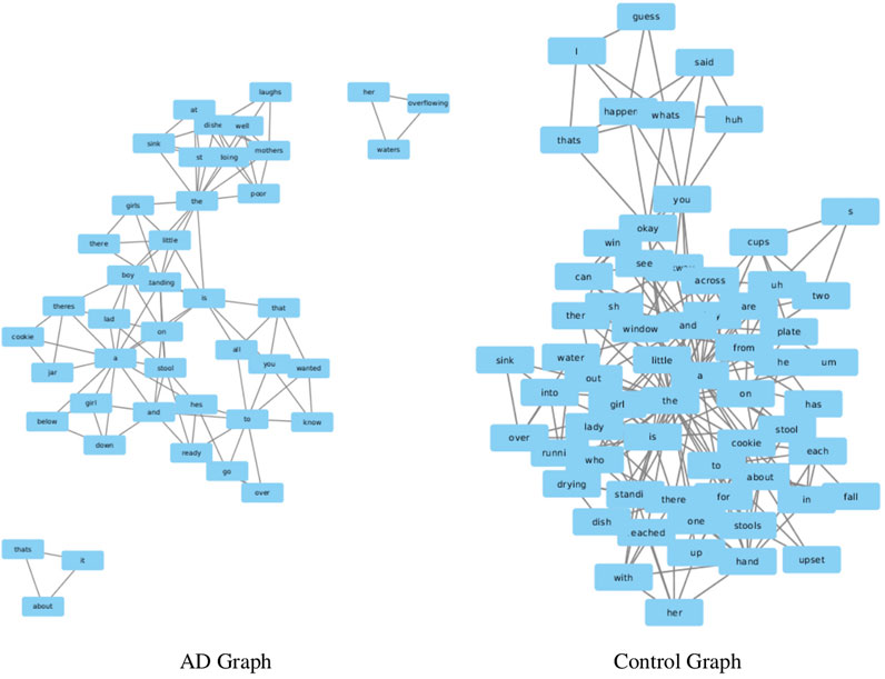
To start with, we show example networks from the control and AD patients in Figure 1. Next we look at the values of various network measures for the co-occurrence networks constructed from the patients and controls. We only use the training set for this analysis. We focus on similar measures to previous work (Liu and Cong (2013)), in this case choosing.

• Number of nodes (N)

• Number of edges (E)

• Edge density (ED)

• Fraction of self links ($SL$)

• Average Clustering Coefficient ($\langle CC\rangle$)

• Diameter (D)

• Heterogeneity (how similar the nodes are to each other)–this is defined as (Estrada, 2010).

$H=\frac{{\displaystyle {\sum }_{i,j\in \Gamma }\left(k_i^{-1/2}-k_j^{-1/2}\right)}}{N-2\sqrt{N-1}},$

where $k_i$ is the degree of node i, $\text{Γ}$ is the edge set.

• Degree Network Centralization $\left(NC\right)$ (how much the network is centered around a small number of highly central nodes) as defined by Freeman (1979).

$NC=\frac{{{\displaystyle {\displaystyle {\sum }_{i=1}^N\left(k_{\text{max}}-k_i\right)}}}^{\text{}}}{N^2-2N+2},$

where $k_i$ is the degree of node i, $k_{\max }$ is the maximum node degree in the graph.

• Average Shortest Path Length ($\langle AV\rangle$)

• Exponent when fitting the degree distribution to a power law (α)

• $x_{\text{min}}$ when fitting the degree distribution to a power law ($x_{\text{min}}$)

• Assortativity (A) (Pearson correlation between the rows of the adjacency matrix)

• Exponent when fitting a power law to the average neighbor degree distribution ($k_{nn}\alpha$)

FIGURE 1

FIGURE 1. Example graphs.

These networks are not connected, and measures that rely on path lengths require modification to be used. In our case the measures that need modifying are the average shortest length path and the diameter. For the average shortest length path, we take the average of all the shortest paths lengths that do exist in the network, discarding those that have infinite length. For the diameter, we take the diameter of the largest component in the graph.

4.2 Results

We show the means of these for each group for a variety of co-occurrence windows (o) in Table 1, where bold font indicates the mean difference is significant according to a Mann-Whitley test at $p<0.05$ for that co-occurrence window. Perhaps unsurprisingly, the measures are affected by the size of the co-occurrence window. Increasing the window size increases the number of edges, and by proxy the edge density. As the network becomes more connected, this increases the average clustering coefficient, network centralization and $x_{\text{min}}$ while decreasing the diameter, heterogeneity, average path length and α. We find that there are six measures with significantly different means for all co-occurrence windows, number of nodes (note this is the same for all window sizes), number of edges, edge density, heterogeneity, network centralization and assortativity. There are three other measures that are significant for one window, fraction of self links and $x_{\text{min}}$ for $o=3$ and $k_{nn}\alpha$ for $o=2$.

TABLE 1

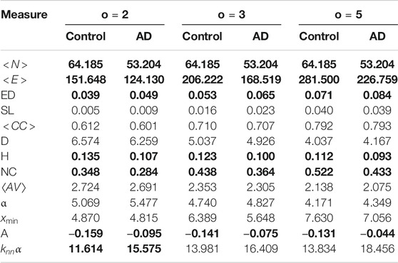
TABLE 1. Means for the network measures for each dataset. Bold font indicates the mean difference is significant between the AD and controls for that co-occurrence window at $p<0.05$ level. The parameter o refers to the size of the co-occurrence window.

Next we look to explain why these measures might be different. Alzheimer’s patients tend to use fewer unique words than controls (Fraser et al., 2016; Orimaye et al., 2018), and tend to repeat words and phrases more frequently than healthy controls. Since unique words correspond to nodes in the graphs, this would explain why controls have a higher number of nodes that those from AD patients, and why the edge density is higher for the AD patients (more edges between a smaller number of nodes). The number of self links should capture word repetitions, and it is higher in the AD networks, but it is notable that it is only significant with a co-occurrence window of 3. For the larger windows there will be more self links overall and proportionally fewer that are due to repetitions, so this could explain why it is not significant for a window of 5.

The AD networks have a lower heterogeneity and a lower network centralization. A lower heterogeneity shows that the degree of the nodes is more equal, while a lower network centralization indicates the network is less orientated around a small number of highly centralized nodes. Furthermore the AD networks are less disassortative than the control networks. A disassortative network is where high degree nodes are connected to low degree nodes, while in an assortative network high degree nodes are connected to other high degree nodes. In general word co-occurrence networks tend to be disassortative (Masucci and Rodgers, 2006; Krishna et al., 2011). We would expect the networks from the AD patients to be smaller, more densely connected and to have a more uniform degree distribution than those from controls, and this seems to be reflected in the graph measures. This would also affect the assortativity of the network–nodes would be less likely to be connected to other nodes of higher degrees, which might indicate greater use of circumlocution in AD networks where disassortativity is reduced.

The average clustering coefficient, diameter and average path length were not significantly different between the AD and controls. We found this surprising as we expected that the average path length and diameter would be shorter for the AD networks as AD patients tend to produce shorter sentences with shorter dependency distances, and the average clustering coefficient larger due to the smaller network size and larger edge density. In fact this is even more surprising as the control networks are larger than the AD networks–so we would expect the diameter and average shortest length path of the control networks to be larger. However, there are disagreements in the literature on whether dependency distance is actually shorter linguistic AD patients’ linguistic output (Pakhomov et al., 2011; Fraser et al., 2016; Orimaye et al., 2017), and average path length is not an exact measure of dependency distance. Furthermore, the transcripts of spontaneous speech used in our experiments are quite short, which might have an effect when comparing these results to results from written text, in the context of which the initial claim was made. It should be noted, however, that recent evidence seems to suggest that dependency lengths in spoken language do not differ significantly to those in written language (Kramer, 2021). Other syntax differences discovered were more node level than global (for instance the number of times the participant utters a pronoun and then an auxiliary verb phase) which cannot be picked up by our measures. The other measures which were not significantly different were $x_{\text{min}}$ and α. These describe the degree distribution of the networks. The lack of significant difference in these measures for the majority of the co-occurrence windows indicates that the networks have a similar degree distribution.

Each transcript is also annotated with an MMSE score, and we look at how this is correlated with the network measures using Spearman correlation. A larger MMSE score indicates the participant is less likely to be in the AD group, so we would expect that graph measures which are larger in the controls to be positively correlated with the MMSE score, and those which are smaller in the controls to be negatively correlation with the MMSE score. The results are shown in Table 2, with significant correlations marked using bold font.

TABLE 2

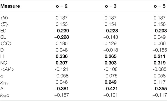
TABLE 2. Spearman Correlation between network measures and MMSE score. Significant correlations are marked with bold font.

There are five measures with significant correlations with the MMSE score, edge density, heterogeneity, network centralization and assortativity. Edge density and assortativity show a negative relationship with the MMSE score, while heterogeneity and network centralization show a positive relationship. Controls have higher MMSE scores than those with AD, so these results mostly reflect the control/AD differences seen above. There are two measures which have a significant difference in means, but do not have significant correlations, the number of nodes and number of edges. This is quite surprising, as these have been shown to be very good predictors of AD. There is a large amount of variance in the MMSE for both classes, so this could be the reason why the mean difference is significant while the correlation is not.

4.3 Comparison to Shuffled Networks

To understand how successful these networks are in capturing the dynamics of word usage we must compare them to a null model. In this section we create null models by shuffling the order of the words for each transcript and constructing networks from these shuffled transcripts. Previous work comparing shuffled networks to their originals has shown that many of the properties of word networks occur to due the frequency of word use rather than due to word order (Caldeira et al., 2006; Krishna et al., 2011).

We create the shuffled networks by randomizing the order of the words in the document. The end of the sentence marker (usually a full-stop) is treated as a word, so sentence structure is not maintained, but the shuffled documents still have sentences. This is done 50 times for each network and then the mean value for each measure is calculated. These are compared to the originals. This allows us to see which structures of the network are due to the frequency of word occurrence and which are due to the specific word order. We show the results of this in Table 3. Again we use a Mann-Whitley test at $p<0.05$ to test for means that are significantly different.

TABLE 3

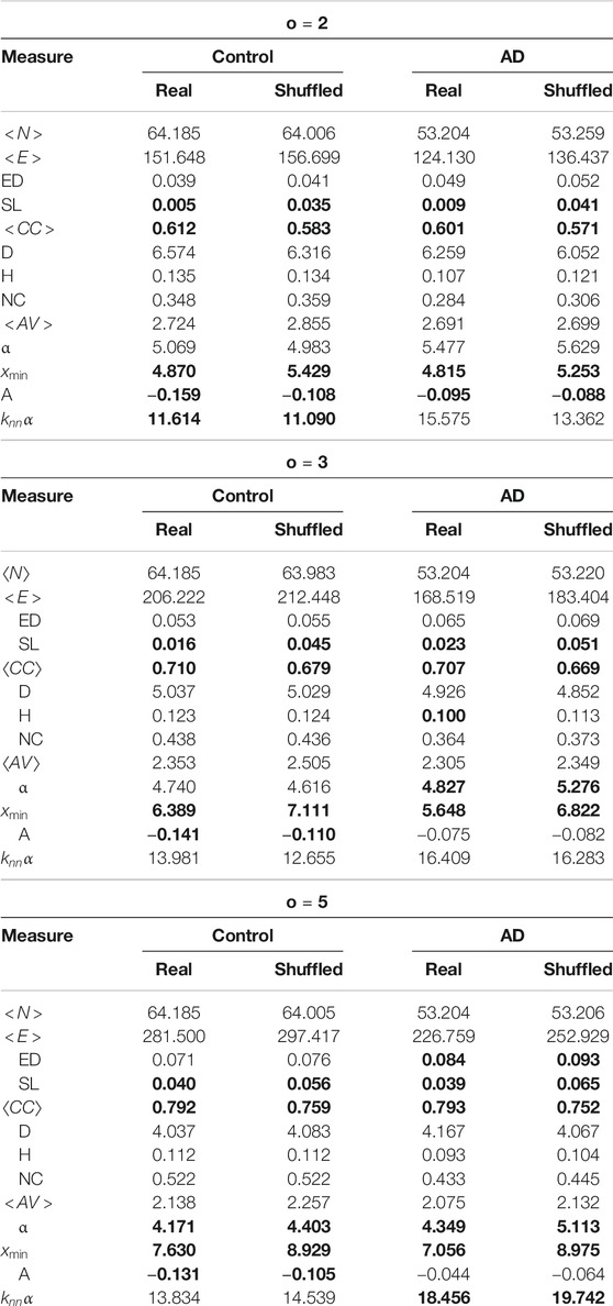
TABLE 3. Comparison of the network measures for the shuffled networks and the real ones. Significant differences are marked with bold font.

Some of the measures are obviously more influenced by the number of words than their order - for instance the number of nodes, number of edges and edge density, and we can see these are not significantly different between the real and shuffled networks for any value. Only the average clustering coefficient, the number of self links and $x_{\text{min}}$ are significantly different between the real and shuffled for all the networks. Assortativity is also different for all the control networks, but only for the co-occurrence window of two for the AD networks.

For the average clustering coefficient, this significant difference is explained by the fact that words co-occur more than would be expected due to random chance. Shuffling destroys this structure, and therefore reduces the clustering coefficient in all of the networks. The difference in self links should also be caused by a similar situation–this measure is clearly influenced by word order, and so should change when this is destroyed. Shuffling also changes the degree structure of the networks, causing changes in the value calculated for $x_{\text{min}}$.

In the previous section we found that there are six network measures that differ between the AD and controls for all co-occurrence windows: number of edges, number of nodes, edge density, heterogeneity, network centralization and assortativity. However out of all of these only assortativity differs between the shuffled and original networks. From a purely network based perspective, it would seem reasonable that assortativity would change between the shuffled and original networks–again we are destroying the co-occurrence structure. Previous work (Krishna et al., 2011) has also confirmed this. However what is surprising is that the difference is significant for controls for all co-occurrence windows, but only for $o=2$ for AD patients. This indicates the AD networks look more random than those from controls.

Previous work has shown that AD patients tend to use more generic terms on picture description tasks than healthy controls, and that the healthy controls use more low frequency content bearing words (Garrard et al., 2014). These two factors help to explain why both heterogeneity and network centralization differ between the AD and controls, but not between the shuffled networks–AD patients will tend to use a smaller set of words, but use each of these words more frequently compared to healthy controls. This indicates that word frequency has the largest impact on the structure of the networks, and we would therefore conclude that word frequency statistics alone would still provide a good feature set to distinguish between the two classes of networks.

5 Transcript Classification

5.1 Method

We are interested in methods for automatic classification of networks into control or AD. This can be done in a variety of ways, with previous work on work co-occurrence networks often using the network measures above as input into a classifier. However there has been a great deal of work in the area of graph classification in the past few years, with many methods being proposed. Generally these methods fall into one of two broad categories: embedding or kernel methods. An embedding method reduces a graph to a vector, while a kernel method learns some kind of similarity measure between graphs and calculates the Gram matrix from this (Kriege et al., 2020). In addition to using the network measures mentioned in the previous section, we also use the spectral features (SF) embedding method created by de Lara and Pineau (2018). This method is based on analyzing the spectrum of the graph’s Laplacian in order to extract a feature vector for the classification algorithm. Firstly we calculate the normalized graph Laplacian

$L=I-D^{-1/2}A{D}^{-1/2},(1)$

where D is the degree matrix, A is the adjacency matrix of the graph and I is the identity matrix. The input into the classifier is then the k smallest eigenvalues of the Laplacian in ascending order

$X=\left({\lambda }_1,{\lambda }_2,\dots {\lambda }_k\right).(2)$

The authors claim that this is similar to classifying a melody by its lowest fundamental frequencies. A deeper explanation of the method is undertaken by Pineau (2019). A larger vector will capture more of the dynamics of the graph, but will also be more prone to overfitting. Since we are not aware of an objective method of selecting k, we experiment with the size of the vector, running for 5, 10, 15, 20 and 50.

A particular emphasis here is that we are not using the word labels in this classification task, but purely the structure of the networks. As mentioned in the previous section, many of the network measures that differ between the AD and controls do not vary between the shuffled and original networks, indicating that many of the differences are due to word frequency usage alone. With this in mind, we use a unigram based method to provide a baseline comparison as to how much word frequency alone can be used to differentiate between the two classes. Here we take the number of different words used and total number of words in the transcript, and then the mean, standard deviation, skew and kurtosis of the distribution of unigrams in the transcript. When creating the distributions of unigrams we only consider the unigrams in the specific transcript. This ensures that we do not leak information across transcripts, and to provide a fairer comparison to the graph measures, as one of the advantages of these graph approaches is that we do not need to consider which words occur in other transcripts.

We use logistic regression (LR), a linear kernel (LSVM), a radial basis function (RBF) kernel (RSVM), and a random forest (RF) to classify the networks. The input variables are standardized to have a mean of 0 and a standard deviation of 1. C for the SVMs is set to 1, and the logistic regression is $L_2$ regularized, with a regularization parameter of 0.5. γ for the RBF kernel is set to $1/p$.

5.2 Results

Firstly we evaluate our approach using leave one out cross-validation (LOOCV) on the training set, and the results are shown in Figure 2. From this we can see that it is possible to distinguish between the co-occurrence networks. We have the highest success at the smallest co-occurrence window of $o=2$ using a linear SVM, with a classification accuracy of 71.3% using the graph measures. Using the graph measures has a higher overall success rate than using the embedding method for every size of co-occurrence window. However the unigram method actually outperforms the network based methods, achieving a maximum accuracy of 73.1% using a linear SVM.

FIGURE 2

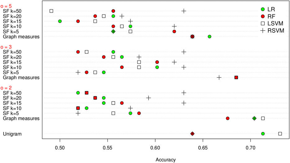
FIGURE 2. Classification accuracy of the unigram, graph measures and SF feature extraction methods on the training set using leave one out cross validation, grouped by co-occurrence window size ($o\in \left\{\mathrm{2,3,5}\right\}$). The best result of 71.3% is achieved using a linear SVM on the graph measures with a co-occurrence window of 2 ($o=2$).

There is not one particular classification algorithm that consistently outperforms the other, with the logistic regression, random forest and linear SVM all having the highest classification accuracy for different co-occurrence window sizes. The co-occurrence window size obviously does not affect the unigram methods. To further evaluate this we use a Wilcoxon signed-rank test to look if the differences in classification accuracy are significant. Again we take $p<0.05$ as a significant difference. To start with we compare the unigram and graph measure feature sets. The only significant difference between them is for the LSVM classifier at $o=5$ (which is the best performing unigram combination against the worst performing graph measures combination), indicating their performance is broadly similar.

Next we compare how the choice of k affects the results for SF. There are some significant differences with the RSVM for $k=5$ with a co-occurrence window of three performing significantly worse than the same classifier for the rest of the values of k, and the different between the RSVM for $k=50,o=5$ performing significantly better than $k=20,o=5$. The rest are not significant, indicating that in general, the choice of k is not particularly important. Comparing the results between the different co-occurrence windows, we find no significant differences for the graph measures. This implies that the choice of co-occurrence window is not particularly important. This again confirms that word frequency seems more important than word co-occurrence.

Looking at the same comparison for SF, there are three classifier/feature sets with a significant difference, logistic regression with $k=10$ between $o=2$ and $o=3$, logistic regression with $k=15$ between $o=3$ and $o=5$ and RSVM with $k=15$ between $o=3$ and $o=5$. Again with the small number of significant differences, we would conclude than the co-occurrence window choice does not particularly affect the SF method.

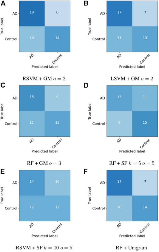
As previously mentioned, the ADReSS dataset contains a pre-tagged test set. Next we look at our success in distinguishing between the AD and control transcripts in the test set. We choose the three best performing classifier/co-occurrence window combinations on the training set for the graph measures, and the two best performing SF methods, in the manner of the ADReSS challenge. The results are shown in Table 4 and confusion matrices in Figure 3. For the combinations that perform the best on the training set, the maximum accuracy achieved is 66.7% using a RSVM classifier with graph measures with graphs that have a co-occurrence window of 2. Bar this outlier though, the accuracy in general has dropped when compared to the results of the leave one out cross-validation on the training set. However, as the test set consists of a very small sample, it is likely that the reported LOOCV accuracy gives a more realistic assessment of the methods we compared.

TABLE 4

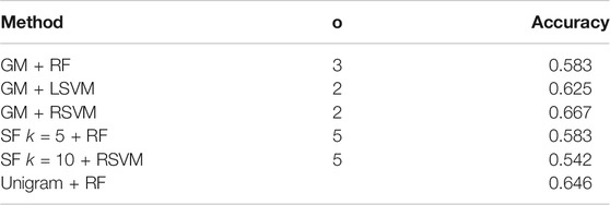
TABLE 4. Classification accuracy of the best performing embedding/classifier combination from the training set on the test set. We choose the three best performing graph measure approaches, the two best SF approaches and the best unigram approach for comparison. There is a decrease in performance in general compared to the training set, but the best performing approach (graph measures with a RSVM classifier) achieves a classification accuracy of 66.7%.

FIGURE 3

FIGURE 3. Confusion matrices for the test set.

Ignoring performance on the training set and purely taking the classifier/feature combination that has the highest performance, we can achieve an accuracy of 75% using a random forest with a co-occurrence window of 2. However since this method did not perform so well on the training set, it is difficult to claim that this is an accurate and reportable classification accuracy.

6 MMSE Prediction

In this section we focus on using the co-occurrence networks to predict the MMSE score for a participant. As with the classification in Section 5, we use the network measures, the SF graph embedding method and the unigram method as features. We choose a set of regression methods analogous to the classification methods chosen above, in this case Linear Regression, Random Forest Regression, and Support Vector Regression with two kernels, a linear kernel and RBF kernel. The input into the regression methods is again standardized so each feature has a mean of 0 and a standard deviation of 1. The predictions are evaluated using root mean squared error (RMSE). C for the SVMs is set to 1, and the linear regression is $L_2$ regularized, with a regularization parameter of 0.5. γ for the RBF kernel is set to $1/p$.

As before, we firstly evaluate the method using LOOCV on the training set. The results are shown in Figure 4. Using a linear regression method with the graph measures appears to obtain the best result (i.e. lowest RMSE), with a RMSE of 4.799 for a co-occurrence window of 2. Again the graph measures seem to give the best results. Following LOOCV, we predict the MMSE of the test set transcripts. As before we take the five embedding/regression combinations that perform the best on the training set and evaluate their performance on the test set. The results are shown in Table 5. Again we do see a decrease in the success of the methods compared to the leave one out evaluation on the training set, with an increase in the RMSE. This time the unigram measures actually give the lowest RMSE, at 5.468, by using linear regression. The best performing graph method uses the graph measures and a random forest regressor with a co-occurrence window of 3, achieving an RMSE of 5.675.

FIGURE 4

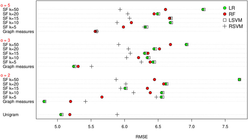
FIGURE 4. RMSE of the unigram, graph measures and SF methods for leave one out cross validation on the training set, grouped by co-occurrence window size ($o\in \left\{\mathrm{2,3,5}\right\}$).

TABLE 5

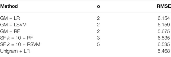
TABLE 5. MMSE of the best performing embedding/regression combination from the training set on the test set. We choose the three best performing graph measure approaches, the two best SF approaches and the best unigram method.

As RMSE values can be difficult to interpret in isolation, we also use the predicted MMSE value to assign the participant as AD or control (a value above 23 indicates a control). The results of this are shown in Table 6. This approach achieves a maximum accuracy of 75% for the graph measures, 64.6% for the unigram methods, and 58.3% for the SF methods. To give a reference, if we use the actual MMSE values for AD prediction, we get an accuracy of 87.5%.

TABLE 6

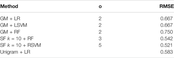
TABLE 6. Accuracy of the best performing regression classifier/embedding methods if we use the predicted MMSE score to predict a transcript as AD or control.

7 Discussion and Conclusion

In this paper we have constructed word co-occurrence networks using transcript data from both controls and Alzheimer’s patients on a picture description task. With these networks we have analyzed some measures of their structure, and used some embedding methods to enable classification of the networks and to predict the MMSE score from the transcript.

Using a Mann-Whitney test we find that there are six measures that have significantly different means between the networks, number of nodes, number of edges, edge density, heterogeneity, network centralization and assortativity. Some of this difference can be explained by previous work in the literature, for instance that AD patients tend to produce fewer unique words and repeat themselves more. Most of these measures also show significant correlation with the MMSE score of the participant. However, many of the measures that differ between the AD and control networks do not differ between the shuffled and original networks. This is unfortunately one of the challenges of using global measures on co-occurrence networks, that in fact many of their properties come from word frequency rather than co-occurrence.

We then looked at classifying the graphs into control or AD using the set of graph measures, and the graph embedding method, SF. Since many of the graph properties come from word frequency and not co-occurrence, we create a baseline feature set using the first four moments of the unigram distribution, plus the total number of unigrams and the number of unique unigrams. We evaluate our success in this firstly by using leave one out cross validation on the training set, and then by using the held back test set from the ADReSS challenge.

In general we find it is possible to classify the networks into control or AD, and that the highest accuracy on the training set is achieved using graph measures and a Linear SVM at 71.3%. For the test set, the highest accuracy achieved is 66.7%, using a RSVM classifier with a co-occurrence window of 2. Using the graph measures gives a higher accuracy than using the SF method, but out of the four classifiers we use, three (Logistic Regression, Random Forest and Linear SVM) have the highest performance at one particular point, making it difficult to recommend the use of one in particular. The same applies to the choice of co-occurrence window. We also find that using the unigram gives fairly comparable results to the graph measures, further indicating that global measures on these word co-occurrence networks mostly reflect word frequency rather than word co-occurrence.

In a similar manner to the graph classification, we also look at predicting the MMSE score from the transcripts. We use the same evaluation methods, leave one out cross validation on the training set, and using the held back test set. On the training set we achieve a minimum RMSE of 4.799 using linear regression and the graph measures with a co-occurrence window of 2, and on the test set we achieve a minimum RMSE of 5.675 using linear regression and the graph measures with a co-occurrence window of 3. Here the unigram methods perform notably better, achieving an RMSE of 5.468 using linear regression. Again the SF method performed poorly compared to the other methods, achieving a maximum accuracy of 6.535 on the test set.

In our work, we have found that using simple unigram measures outperforms using more complex graph based measures which should take co-occurrence into account. However, looking at the features that previous work has found to be useful in distinguishing between AD and control patients, it could be that the measures we have chosen cannot capture these differences with a great deal with success. Combined with previous work showing that global network measures on word co-occurrence networks struggle to capture word order, we would suggest that future work either relies node level measures, or devises novel global measures that can capture word order. We also note that our network-based approach performed comparably to the ADReSS baseline, with scores of 5.68 vs 5.20 RMSE for regression, and 66.7% vs 75.0% for classification (Luz et al., 2020). However, none of the participants employed a network based approach.

Data Availability Statement

Publicly available datasets were analyzed in this study. This data can be found here: https://dementia.talkbank.org/. Instructions on how to acquire the dataset are available at https://edin.ac/375QRNI. The source code for the experiments described in this paper is available at https://git.ecdf.ed.ac.uk/tmilling/analysis-and-classification-of-word-co-occurrence-networks.

Author Contributions

TM and SL conceived and designed the experiments and analysis. SL prepared the dataset. TM implemented the network-generation and feature extraction algorithms, performed analysis and drafted the manuscript. Both authors contributed to the final version of the manuscript.

Funding

This work funded by the European Union’s Horizon 2020 research and∼innovation program, under the grant agreement No 769661, toward the SAAM project.

Conflict of Interest

The authors declare that the research was conducted in the absence of any commercial or financial relationships that could be construed as a potential conflict of interest.

Footnotes

¹https://git.ecdf.ed.ac.uk/tmilling/analysis-and-classification-of-word-co-occurrence-networks

²https://edin.ac/375QRNI

References

Akimushkin, C., Amancio, D. R., and Oliveira, O. N. (2017). Text Authorship Identified Using the Dynamics of Word Co-Occurrence Networks. PloS one 12, e0170527. doi:10.1371/journal.pone.0170527

PubMed Abstract | CrossRef Full Text | Google Scholar

Alberdi, A., Weakley, A., Schmitter-Edgecombe, M., Cook, D. J., Aztiria, A., Basarab, A., et al. (2018). Smart Home-Based Prediction of Multidomain Symptoms Related to Alzheimer’s Disease. IEEE J. Biomed. Health Inform. 22, 1720–1731. doi:10.1109/jbhi.2018.2798062

PubMed Abstract | CrossRef Full Text | Google Scholar

Amancio, D. R., Antiqueira, L., Pardo, T. A. S., da F. COSTACosta, L. L., Oliveira, O. N., and Nunes, M. G. V. (2008). Complex Networks Analysis of Manual and Machine Translations. Int. J. Mod. Phys. C 19, 583–598. doi:10.1142/S0129183108012285

CrossRef Full Text | Google Scholar

Amancio, D. R. (2015). Comparing the Topological Properties of Real and Artificially Generated Scientific Manuscripts. Scientometrics 105, 1763–1779. doi:10.1007/s11192-015-1637-z

CrossRef Full Text | Google Scholar

Antiqueira, L., Pardo, T. A. S., Nunes, M. d. G. V., and Oliveira, O. N. (2007). Some Issues on Complex Networks for Author Characterization. Inteligencia Artificial. Revista Iberoamericana de Inteligencia Artif. 11, 51–58. doi:10.4114/ia.v11i36.891

CrossRef Full Text | Google Scholar

Barrenechea, J., Bullmore, E., and Plenz, D. (2014). Powerlaw: A python Package for Analysis of Heavy-Tailed Distributions. PLoS One 9, e85777–e857711. doi:10.1371/journal.pone.0085777

PubMed Abstract | CrossRef Full Text | Google Scholar

Becker, J. T., Boiler, F., Lopez, O. L., Saxton, J., and McGonigle, K. L. (1994). The Natural History of Alzheimer’s Disease. Arch. Neurol. 51, 585–594. doi:10.1001/archneur.1994.00540180063015

PubMed Abstract | CrossRef Full Text | Google Scholar

Bougouin, A., Boudin, F., and Daille, B. (2013). “TopicRank: Graph-Based Topic Ranking for Keyphrase Extraction,” in Proceedings of the Sixth International Joint Conference on Natural Language Processing. Nagoya, Japan: Asian Federation of Natural Language Processing, 543–551.

Google Scholar

Caldeira, S. M. G., Petit Lobão, T. C., Andrade, R. F. S., Neme, A., and Miranda, J. G. V. (2006). The Network of Concepts in Written Texts. Eur. Phys. J. B 49, 523–529. doi:10.1140/epjb/e2006-00091-3

CrossRef Full Text | Google Scholar

Cancho, R. F. i., and Solé, R. V. (2001). The Small World of Human Language. Proc. R. Soc. Lond. B 268, 2261–2265. doi:10.1098/rspb.2001.1800

CrossRef Full Text | Google Scholar

Cong, J., and Liu, H. (2014). Approaching Human Language with Complex Networks. Phys. Life Rev. 11, 598–618. doi:10.1016/j.plrev.2014.04.004

PubMed Abstract | CrossRef Full Text | Google Scholar

de la Fuente Garcia, S., Ritchie, C., and Luz, S. (2020). Artificial Intelligence, Speech, and Language Processing Approaches to Monitoring Alzheimer’s Disease: A Systematic Review. J. Alzheimer’s Dis. 78, 1547–1574. doi:10.3233/JAD-200888

CrossRef Full Text | Google Scholar

de Lara, N., and Pineau, E. (2018). A Simple Baseline Algorithm for Graph Classification. Available at: https://arxiv.org/abs/1810.09155.

Google Scholar

Estrada, E. (2010). Quantifying Network Heterogeneity. Phys. Rev. E 82, 066102. doi:10.1103/physreve.82.066102

PubMed Abstract | CrossRef Full Text | Google Scholar

Florescu, C., and Caragea, C. (2017). “PositionRank: An Unsupervised Approach to Keyphrase Extraction from Scholarly Documents,” in Proceedings of the 55th Annual Meeting of the Association for Computational Linguistics (Vancouver, Canada: Association for Computational Linguistics) 1, 1105–1115. doi:10.18653/v1/P17-1102

CrossRef Full Text | Google Scholar

Fraser, K. C., Meltzer, J. A., and Rudzicz, F. (2016). Linguistic Features Identify Alzheimer’s Disease in Narrative Speech. J. Alzheimers Dis. 49, 407–2210. doi:10.3233/JAD-150520

PubMed Abstract | CrossRef Full Text | Google Scholar

Freeman, L. C. (1979). Centrality in Social Networks I: Conceptual Clarification. Social Networks 1, 215–239. doi:10.1016/0378-8733(78)90021-7

CrossRef Full Text | Google Scholar

Garrard, P., Maloney, L. M., Hodges, J. R., and Patterson, K. (2005). The Effects of Very Early Alzheimer’s Disease on the Characteristics of Writing by a Renowned Author. Brain 128, 250–6010. doi:10.1093/brain/awh341

PubMed Abstract | CrossRef Full Text | Google Scholar

Garrard, P., Rentoumi, V., Gesierich, B., Miller, B., and Gorno-Tempini, M. L. (2014). Machine Learning Approaches to Diagnosis and Laterality Effects in Semantic Dementia Discourse. Cortex 55, 122–129. doi:10.1016/j.cortex.2013.05.008

PubMed Abstract | CrossRef Full Text | Google Scholar

Hagberg, A. A., Schult, D. A., and Swart, P. J. (2008). “Exploring Network Structure, Dynamics, and Function Using Networkx,” in Proceedings of the 7th Python in Science Conference. Pasadena, CA, 11–15. doi:10.25080/issn.2575-9752

CrossRef Full Text | Google Scholar

Haider, F., De La Fuente, S., and Luz, S. (2020). An Assessment of Paralinguistic Acoustic Features for Detection of Alzheimer’s Dementia in Spontaneous Speech. IEEE J. Sel. Top. Signal. Process. 14, 272, 281. doi:10.1109/JSTSP.2019.2955022

CrossRef Full Text | Google Scholar

Hassan, S., Mihalcea, R., and Banea, C. (2007). Random Walk Term Weighting for Improved Text Classification. Int. J. Semantic Comput. 01, 421–439. doi:10.1142/s1793351x07000263

CrossRef Full Text | Google Scholar

Hunter, J. D. (2007). Matplotlib: A 2d Graphics Environment. Comput. Sci. Eng. 9, 90–95. doi:10.1109/MCSE.2007.55

CrossRef Full Text | Google Scholar

Kramer, A. (2021). Dependency Lengths in Speech and Writing: A Cross-Linguistic Comparison via Youdepp, a Pipeline for Scraping and Parsing Youtube Captions. Proc. Soc. Comput. Linguistics 4, 359–365.

Google Scholar

Kriege, N. M., Johansson, F. D., and Morris, C. (2020). A Survey on Graph Kernels. Appl. Netw. Sci. 5, 1–42. doi:10.1007/s41109-019-0195-3

CrossRef Full Text | Google Scholar

Krishna, M., Hassan, A., Liu, Y., and Radev, D. (2011). The Effect of Linguistic Constraints on the Large Scale Organization of Language. Available at: https://arxiv.org/abs/1102.2831.

Google Scholar

Lee, J. L., Burkholder, R., Flinn, G. B., and Coppess, E. R. (2016). Working with CHAT Transcripts in Python. Tech. Rep. TR-2016-02. Department of Computer Science, University of Chicago.

Google Scholar

Liu, H., and Cong, J. (2013). Language Clustering with Word Co-occurrence Networks Based on Parallel Texts. Chin. Sci. Bull. 58, 1139–1144. doi:10.1007/s11434-013-5711-8

CrossRef Full Text | Google Scholar

Loper, E., and Bird, S. (2002). “NLTK: The Natural Language Toolkit,” in Proceedings of the ACL-02 Workshop on Effective Tools and Methodologies for Teaching Natural Language Processing and Computational Linguistics - 1. Philadelphia, PA: Association for Computational Linguistics, 63–70. doi:10.3115/1118108.1118117

CrossRef Full Text | Google Scholar

Luz, S., de la Fuente, S., and Albert, P. (2018). A Method for Analysis of Patient Speech in Dialogue for Dementia Detection. Available at: http://arxiv.org/abs/1811.09919.

Google Scholar

Luz, S., Haider, F., de la Fuente, S., Fromm, D., and MacWhinney, B. (2020). “Alzheimer’s Dementia Recognition through Spontaneous Speech: The ADReSS Challenge,” in Proceedings of INTERSPEECH 2020. doi:10.21437/interspeech.2020-2571

CrossRef Full Text | Google Scholar

MacWhinney, B. (2019). Understanding Spoken Language through Talkbank. Behav. Res. 51, 1919–1927. doi:10.3758/s13428-018-1174-9

PubMed Abstract | CrossRef Full Text | Google Scholar

Masucci, A. P., and Rodgers, G. J. (2006). Network Properties of Written Human Language. Phys. Rev. E 74, 026102. doi:10.1103/PhysRevE.74.026102

PubMed Abstract | CrossRef Full Text | Google Scholar

McKinney, W. (2010). “Data Structures for Statistical Computing in python,” in Proceedings of the 9th Python in Science Conference. Editors S. van der Walt, and J. Millman, 51–56. doi:10.25080/issn.2575-9752

CrossRef Full Text | Google Scholar

Mehri, A., Darooneh, A. H., and Shariati, A. (2012). The Complex Networks Approach for Authorship Attribution of Books. Physica A: Stat. Mech. its Appl. 391, 2429–2437. doi:10.1016/j.physa.2011.12.011

CrossRef Full Text | Google Scholar

Mihalcea, R., and Tarau, P. (2004). “Textrank: Bringing Order into Text,” in Proceedings of the 2004 conference on empirical methods in natural language processing. 404–411. doi:10.3115/1220355.1220517

CrossRef Full Text | Google Scholar

Oliphant, T. E. (2006). A guide to NumPy. Scotts Valley, CA: CreateSpace..

Orimaye, S. O., Wong, J. S.-M., and Wong, C. P. (2018). Deep Language Space Neural Network for Classifying Mild Cognitive Impairment and Alzheimer-type Dementia. PLoS One 13, e0205636–15. doi:10.1371/journal.pone.0205636

PubMed Abstract | CrossRef Full Text | Google Scholar

Orimaye, S. O., Wong, J. S., Golden, K. J., Wong, C. P., and Soyiri, I. N. (2017). Predicting Probable Alzheimer’s Disease Using Linguistic Deficits and Biomarkers. BMC bioinformatics 18, 34. doi:10.1186/s12859-016-1456-0

PubMed Abstract | CrossRef Full Text | Google Scholar

Pakhomov, S., Chacon, D., Wicklund, M., and Gundel, J. (2011). Computerized Assessment of Syntactic Complexity in Alzheimer's Disease: a Case Study of Iris Murdoch's Writing. Behav. Res. 43, 136–144. doi:10.3758/s13428-010-0037-9

PubMed Abstract | CrossRef Full Text | Google Scholar

Pedregosa, F., Varoquaux, G., Gramfort, A., Michel, V., Thirion, B., Grisel, O., et al. (2011). Scikit-learn: Machine Learning in python. J. Machine Learn. Res. 12, 2825–2830.

Google Scholar

Pineau, E. (2019). Using Laplacian Spectrum as Graph Feature Representation. Available at: http://arvix.org/abs/1912.00735.

Google Scholar

Rousseau, F., Kiagias, E., and Vazirgiannis, M. (2015). “Text Categorization as a Graph Classification Problem,” in Proceedings of the 53rd Annual Meeting of the Association for Computational Linguistics and the 7th International Joint Conference on Natural Language Processing (Beijing, China: Association for Computational Linguistics)) 1, 1702–1712. doi:10.3115/v1/P15-1164

CrossRef Full Text | Google Scholar

Rozemberczki, B., Kiss, O., and Sarkar, R. (2020). An Api Oriented Open-Source python Framework for Unsupervised Learning on Graphs. Available at: http://arvix.org/abs/2003.04819..

CrossRef Full Text | Google Scholar

Santos, L. B. d., Corrêa, E. A., Oliveira, O. N., Amancio, D. R., Mansur, L. L., and Aluísio, S. M. (2017). Enriching Complex Networks with Word Embeddings for Detecting Mild Cognitive Impairment from Speech Transcripts. Available at: https://arxiv.org/abs/1704.08088..

CrossRef Full Text | Google Scholar

Shannon, P., Markiel, A., Ozier, O., Baliga, N. S., Wang, J. T., Ramage, D., et al. (2003). Cytoscape: a Software Environment for Integrated Models of Biomolecular Interaction Networks. Genome Res. 13, 2498–2504. doi:10.1101/gr.1239303

PubMed Abstract | CrossRef Full Text | Google Scholar

Slegers, A., Filiou, R.-P., Montembeault, M., and Brambati, S. M. (2018). Connected Speech Features from Picture Description in Alzheimer’s Disease: A Systematic Review. Jad 65, 519–542. doi:10.3233/jad-170881

PubMed Abstract | CrossRef Full Text | Google Scholar

Wankerl, S., Nöth, E., and Evert, S. (2017). An N-Gram Based Approach to the Automatic Diagnosis of Alzheimer’s Disease from Spoken Language. INTERSPEECH, 3162–3166. doi:10.21437/Interspeech.2017-1572

Google Scholar

Yan, X., and Han, J. (2002). “Gspan: Graph-Based Substructure Pattern Mining,” in IEEE International Conference on Data MiningProceedings. IEEE, 721–724.

Google Scholar