FusionNet: A Deep Fully Residual Convolutional Neural Network for Image Segmentation in Connectomics

Cellular-resolution connectomics is an ambitious research direction with the goal of generating comprehensive brain connectivity maps using high-throughput, nano-scale electron microscopy. One of the main challenges in connectomics research is developing scalable image analysis algorithms that require minimal user intervention. Deep learning has provided exceptional performance in image classification tasks in computer vision, leading to a recent explosion in popularity. Similarly, its application to connectomic analyses holds great promise. Here, we introduce a deep neural network architecture, FusionNet, with a focus on its application to accomplish automatic segmentation of neuronal structures in connectomics data. FusionNet combines recent advances in machine learning, such as semantic segmentation and residual neural networks, with summation-based skip connections. This results in a much deeper network architecture and improves segmentation accuracy. We demonstrate the performance of the proposed method by comparing it with several other popular electron microscopy segmentation methods. We further illustrate its flexibility through segmentation results for two different tasks: cell membrane segmentation and cell nucleus segmentation.

1 Introduction

The brain is considered the most complex organ in the human body. Despite decades of intense research, our understanding of how its structure relates to its function remains limited (Lichtman and Denk, 2011). Connectomics research seeks to disentangle the complicated neuronal circuits embedded within the brain. This field has gained substantial attention recently thanks to the advent of new serial-section electron microscopy (EM) technologies (Briggman and Bock, 2012; Hayworth et al., 2014; Eberle and Zeidler, 2018; Zheng et al., 2018; Graham et al., 2019). The resolution afforded by EM is sufficient for resolving tiny but important neuronal structures that are often densely packed together, such as dendritic spine necks and synaptic vesicles. These structures are often only tens of nanometers in diameter (Helmstaedter, 2013). Figure 1 shows an example of such an EM image and its cell membrane segmentation. Such high-resolution imaging results in enormous datasets, approaching one petabyte for only the relatively small tissue volume of one cubic millimeter. Therefore, handling and analyzing EM datasets is one of the most challenging problems in connectomics.

FIGURE 1

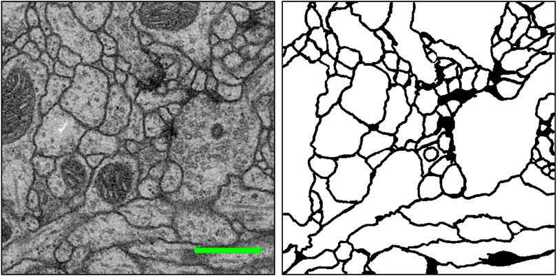
FIGURE 1. An example EM image (left) and its manually extracted cellular membrane segmentation result (right) from the ISBI 2012 EM segmentation challenge (Arganda-Carreras et al., 2015). Scale bar (green): 500 nm.

Early connectomics research focused on the sparse reconstruction of neuronal circuits (Bock et al., 2011; Briggman et al., 2011), meaning they focused reconstruction efforts on a subset of neurons in the data using manual or semi-automatic tools (Jeong et al., 2010; Sommer et al., 2011; Cardona et al., 2012). Unfortunately, this approach requires too much human interaction to scale well over the vast amount of EM data that can be collected with new technologies. Therefore, developing scalable and automatic image analysis algorithms is an important and active research direction in the field of connectomics.

Although some EM image processing pipelines use conventional, light-weight pixel classifiers [e.g., RhoANA (Kaynig et al., 2015)], the majority of automatic image segmentation algorithms for connectomics rely on deep learning. Earlier automatic segmentation work using deep learning mainly focused on patch-based pixel-wise classification based on a convolutional neural network (CNN) for affinity map generation (Turaga et al., 2010) and cell membrane probability estimation (Ciresan et al., 2012). However, one limitation of applying a conventional CNN to EM image segmentation is that per-pixel network deployment scaling becomes prohibitively expensive considering the tera-scale to peta-scale EM data size. For this reason, more efficient and scalable deep neural networks are important for image segmentation of the large datasets that can now be produced. One approach is to extend a fully convolutional neural network (FCN) (Long et al., 2015), which uses encoding and decoding phases similar to an autoencoder for the end-to-end semantic segmentation problem (Ronneberger et al., 2015; Chen et al., 2016a).

The motivation of the proposed work stems from our recent research effort to develop a deeper neural network for end-to-end cell segmentation with higher accuracy. We observed that, like conventional CNNs, a popular deep neural network for end-to-end segmentation known as U-net (Ronneberger et al., 2015) is limited by gradient vanishing with increasing network depth. To address this problem, we propose two extensions of U-net: using residual layers in each level of the network and introducing summation-based skip connections to make the entire network much deeper. Our segmentation method produces an accurate result that is competitive with similar EM segmentation methods. The main contribution of this study can be summarized as follows:

• We introduce an end-to-end automatic EM image segmentation method using deep learning. The proposed method combines a variant of U-net and residual CNN with novel summation-based skip connections to make the proposed architecture, a fully residual deep CNN. This new architecture directly employs residual properties within and across levels, thus providing a deeper network with higher accuracy.

• We demonstrate the performance of the proposed deep learning architecture by comparing it with several EM segmentation methods listed in the leader board of the ISBI 2012 EM segmentation challenge (Arganda-Carreras et al., 2015). Our method outperformed many of the top-ranked methods in terms of segmentation accuracy.

• We introduce a data enrichment method specifically built for EM data by collecting all the orientation variants of the input images (eight in the 2D case, including all combinations of flipping and rotation). We used the same augmentation process for deployment: the final output is a combination of eight different probability values, which increases the accuracy of the method.

• We demonstrate the flexibility of the proposed method on two different EM segmentation tasks. The first involves cell membrane segmentation on a fruit fly (Drosophila) EM dataset (Arganda-Carreras et al., 2015). The second involves cell nucleus feature segmentation on a whole-brain larval zebrafish EM dataset (Hildebrand et al., 2017).

2 Related Work

Deep neural networks (LeCun et al., 2015) have surpassed human performance in solving many complex visual recognition problems. Systems using this method can flexibly learn to recognize patterns such as handwritten digits (Krizhevsky et al., 2012) in images with increasing layers hierarchically corresponding to increasing feature complexity (Zeiler and Fergus, 2014). A major drawback of using deep neural networks is that they often require a huge amount of training data. In order to overcome this issue, researchers have started to collect large databases containing millions of images that span hundreds of categories (Russakovsky et al., 2015). Largely thanks to such training datasets, many advanced architectures have been introduced, including VGG (Simonyan and Zisserman, 2014) and GoogleNet (Szegedy et al., 2015). With these architectures, computers are now able to perform even more complex tasks, such as transferring artistic styles from a source image to an unrelated target (Gatys et al., 2016). To leverage these new capabilities, researchers are actively working to extend deep learning methods for analyzing biomedical image data (Cicek et al., 2016). Developing such methods for automatic classification and segmentation of different biomedical image modalities, such as CT (Zheng et al., 2015) and MRI (Isin et al., 2016), is leading to faster and more accurate decision-making processes in laboratory and clinical settings.

Similarly, deep learning has been quickly adopted by connectomics researchers to enhance automatic EM image segmentation. One of the earliest applications to EM segmentation involved the straightforward application of a convolutional neural network (CNN) for pixel-wise membrane probability estimation (Ciresan et al., 2012), an approach that won the ISBI 2012 EM segmentation challenge (Arganda-Carreras et al., 2015). As more deep learning methods are introduced, automatic EM segmentation techniques evolve and new groups overtake the title of state-of-the-art performance in such challenges. One notable recent advancement was the introduction of a fully convolutional neural network (FCN) (Long et al., 2015) for end-to-end semantic segmentation. Inspired by this work, several modified FCNs have been proposed for EM image segmentation. One variant combined multi-level upscaling layers to produce a final segmentation (Chen et al., 2016a). Additional post-processing steps such as lifted multi-cut (Beier et al., 2016; Pape et al., 2019) further refined this segmentation result.

Another approach added skip connections for concatenating feature maps into a “U-net” architecture (Ronneberger et al., 2015). While U-net and its variants can learn multi-contextual information from input data, they are limited in the depth of the network they can construct because of the vanishing gradient problem. On the other hand, the addition of shortcut connections and direction summations (He et al., 2016) allows gradients to flow across multiple layers during the training phase. This creates a fully residual CNN where the architecture is a fusion of the U-net design and networks with summation-based skip connections, similar to Fully Convolutional Residual Networks (FC-ResNets) (Drozdzal et al., 2016) and Residual Deconvolutional Networks (RDN) (Fakhry et al., 2017). These related studies inspired us to propose a fully residual CNN for analyzing connectomics data.

Work that leverages recurrent neural network (RNN) architectures can also accomplish this segmentation task (Stollenga et al., 2015). Instead of simultaneously considering all surrounding pixels and computing responses for the feature maps, RNN-based networks treat the pixels as a list or sequence with various routing rules and recurrently update each feature pixel. In fact, RNN-based membrane segmentation approaches are crucial for connected component labeling steps that can resolve false splits and merges during the post-processing of probability maps (Ensafi et al., 2014; Parag et al., 2015).

3 Methods

3.1 Network Architecture

Our proposed network, FusionNet, is based on the architecture of a convolutional autoencoder and is illustrated in Figure 2. It consists of an encoding path (upper half, from 640 × 640 to 40 × 40) that retrieves features of interest and a symmetric decoding path (lower half, from 40 × 40 to 640 × 640) that accumulates the feature maps from different scales to form the segmentation. Both the encoding and decoding paths consist of multiple levels (i.e., resolutions). Four basic building blocks are used to construct the proposed network. Each green block is a regular convolutional layer followed by rectified linear unit activation and batch normalization (omitted from the figure for simplicity). Each violet block is a residual layer that consists of three convolutional blocks and a residual skip connection. Each blue block is a maxpooling layer located between levels only in the encoding path to perform downsampling for feature compression. Each red block is a deconvolutional layer located between levels only in the decoding path to upsample the input data using learnable interpolations. A detailed specification of FusionNet, including the number of feature maps and their sizes, is provided in Table 1.

FIGURE 2

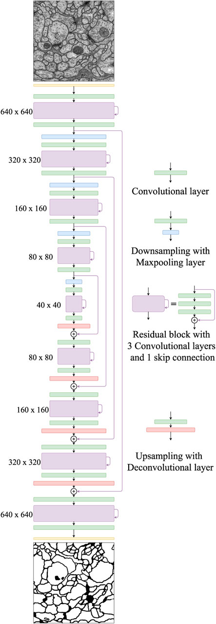
FIGURE 2. The proposed FusionNet architecture. An illustration of the encoding path (top to middle) and the decoding path (middle to bottom). Each intermediate residual block contains a residual skip connection within the same path, while the nested residual skip connections connect two different paths.

TABLE 1

TABLE 1. Architecture of the proposed network.

One major difference between the FusionNet and U-net architectures is the way in which skip connections are used (Figure 3). In FusionNet, each level in the decoding path begins with a deconvolutional block (red) that un-pools the feature map from a coarser level (i.e., resolution), then merges it by pixel-wise addition with the feature map from the corresponding level in the encoding path by a long skip connection. There is also a short skip connection contained in each residual block (violet) that serves as a direct connection from the previous layer within the same encoding or decoding path. In contrast, U-net concatenates feature maps using only long skip connections. Additionally, by replacing concatenation with addition, FusionNet becomes a fully residual network, which resolves some common issues in deep networks (i.e., gradient vanishing). Furthermore, the nested short and long skip connections in FusionNet permit information flow within and across levels.

FIGURE 3

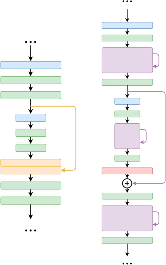
FIGURE 3. Difference between the core connections of U-net (Ronneberger et al., 2015) (left) and FusionNet (right). Note that FusionNet is a fully residual network due to the summation-based skip connections and is a much deeper network.

In the FusionNet encoding path, the number of feature maps doubles whenever downsampling is performed. After passing through the encoding path, the bridge level (i.e., 40 × 40 layer) residual block starts to expand feature maps into the following decoding path. In the decoding path, the number of feature maps is halved at every level, which maintains network symmetry. Note that there are convolutional layers both before and after each residual block. These convolutional layers serve as portal gateways that effectively adjust the amount of feature maps before and after residual blocks to the appropriate numbers. The placement of these convolutional layers on either side of the residual block leads the entire network to be perfectly symmetric (see Figure 2).

FusionNet performs end-to-end segmentation from the input EM data to the output segmentation label prediction. We train the network with pairs of EM images and their corresponding manually segmented label images as input. The training process involves comparing the output prediction with the input target labels using a mean-absolute-error (MAE) loss function to back-propagate adjustments to the connection weights. We considered the network sufficiently trained when its loss function values plateaued over several hundred epochs.

3.2 Data Augmentation

Our system involves data augmentation in multiple stages during both the training and deployment phases.

For training:

• The order of the image and label pairs are shuffled and organized with three-fold cross-validation to improve the generalization of our method.

• Offline, all training images and labels are reoriented to first produce an enriched dataset.

• Online, elastic field deformation is applied to both images and corresponding labels, followed by noise addition to only the images.

For prediction:

• Offline, input images are reoriented as for training.

• Inference is performed on all reoriented images separately, then each intermediate result is reverted to the original orientation, and all intermediate results are averaged to produce the final prediction.

Boundary extension is performed for all input images and labels. We describe each augmentation step in more detail in the following subsections.

Reorienation enrichment: Different EM images typically share similar orientation-independent textures in structures such as mitochondria, axons, and synapses. We reasoned that it should therefore be possible to enrich our input data with seven additional image and label pairs by reorienting the EM images, and in the case of training, their corresponding labels. Figure 4 shows all eight orientations resulting from a single EM image after performing this data enrichment, with an overlaid letter “g” in each panel to provide a simpler view of the generated orientation. To generate these permutations, we rotated each EM image (and corresponding label) by 90°, 180°, and 270°. We then vertically reflected the original and rotated images. For training, each orientation was added as a new image and label pair. For prediction, inference was performed on each of these data orientations separately, then each prediction result was reverted to the original orientation before averaging to produce the final accumulation. Our intuition here is that, based on the equivariance of isotropic data, each orientation will contribute equally toward the final prediction result. Note that because the image and label pairs are enriched eight times by this process, other on-the-fly linear data augmentation techniques such as random rotation, flipping, or transposition are unnecessary.

FIGURE 4

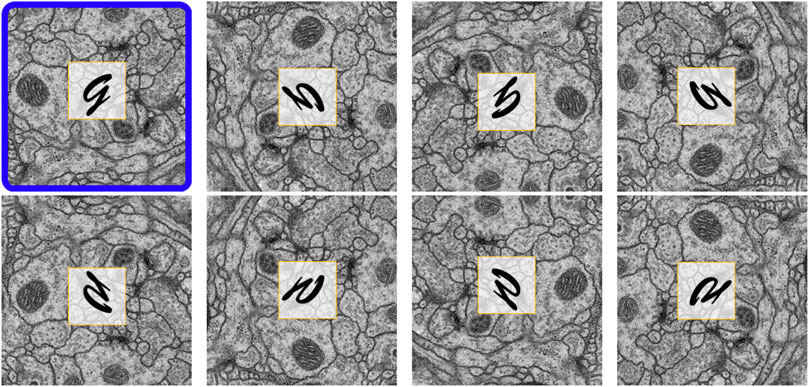
FIGURE 4. Eight reoriented versions of the same EM image. The original image is outlined in blue. By adding these reoriented images, the input data size is increased by eight times.

Elastic field deformation: To avoid overfitting (i.e., network remembering the training data), elastic deformation was performed on the entire enriched image dataset for every training epoch. This strategy is common in machine learning, especially for deep networks, to overcome limitations associated with small training dataset sizes. This procedure is illustrated in Figure 5. We first initialized a random sparse 12 × 12 vector field whose amplitudes at the image border boundaries vanish to zero. This field was then interpolated to the input size and used to warp both EM images and corresponding labels. The flow map was randomly generated for each epoch. No elastic field deformation was performed during deployment.

FIGURE 5

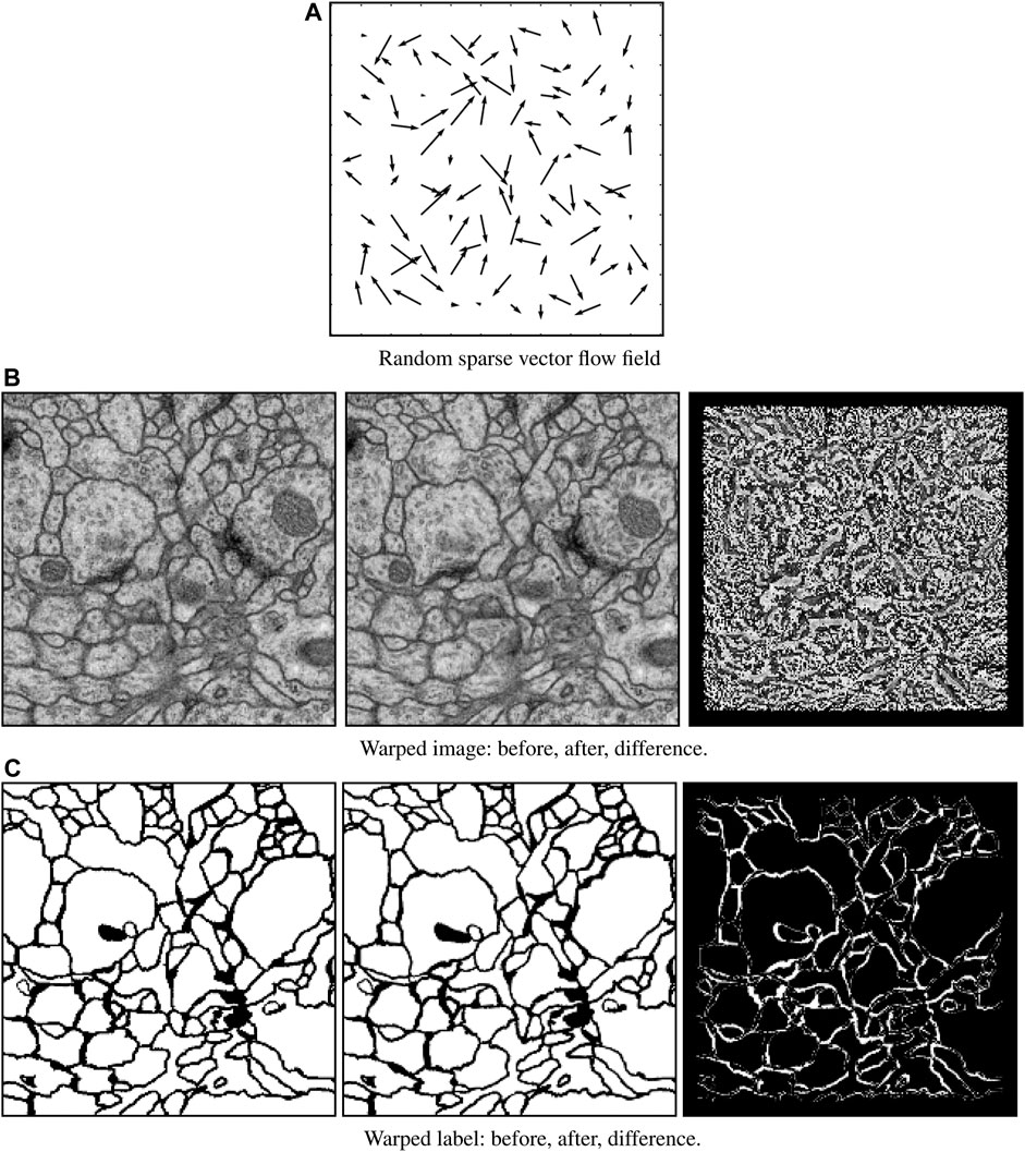
FIGURE 5. Elastic field deformation example. A randomly sparse vector field (A) is generated for each training image and label pair. This sparse vector field is then used to warp both the original image data (B, left) and its corresponding label (C, left) to form an augmentation pair consisting of warped image data (B, middle) and warped label (C, middle). The difference between the original and warped images (B, right) and labels (C, right) show the effect of deformation.

Random noise addition: During only the training phase, we randomly added Gaussian noise (mean µ = 0, variance $\sigma =0.1$) to each EM input image but not its corresponding label.

Boundary extension: FusionNet accepts an input image size of 512 × 512. Each input image, and in the case of training its corresponding label, was automatically padded with the mirror reflections of itself across the image border boundary (radius = 64 px) to maintain similar statistics for pixels that are near the edges. This padding is the reason why FusionNet starts with a 640 × 640 image, which is 128 px larger along each edge than the original input. However, we performed convolution with 3 × 3 kernel size and “SAME” mode, which leads the final segmentation to have the same padded size. To account for this, the final output prediction was cropped to eliminate the padded regions.

3.3 Experimental Setup

FusionNet was implemented using the Keras open-source deep learning library (Chollet, 2015). This library provides an easy-to-use, high-level programming API written in Python, with Theano or TensorFlow as a back-end engine. The model was trained with the Adam optimizer with a decaying learning rate of 2e⁻⁴ for over 50,000 epochs to harness the benefits of heavy elastic deformation on the small annotated datasets. FusionNet has also been translated to PyTorch and pure TensorFlow for other applications, such as Image-to-Image translation (Lee et al., 2018) and MRI reconstruction (Quan et al., 2018). All training and deployment presented here was conducted on a system with an Intel i7 CPU, 32 GB RAM, and a NVIDIA GTX GeForce 1080 GPU.

3.4 Network Chaining

FusionNet by itself performs end-to-end segmentation from the EM data input to the final prediction output. In typical real world applications of end-to-end segmentation approaches, however, manual proofreading by human experts is usually performed in an attempt to “correct” any mistakes in the output labels. We therefore reasoned that concatenating a chain of several FusionNet units could serve as a form of built-in refinement similar to proofreading that could resolve ambiguities in the initial predictions. Figure 6 shows an example case with four chained FusionNet units (FusionNetW⁴). To impose a target-driven approach across the chained network during training, we calculate the loss between the output of each separate unit and the training labels. As a result, chained FusionNet architectures have a single input and multiple outputs, where the end of each decoding path serves as a checkpoint between units attempting to produce better and better segmentation results.

FIGURE 6

FIGURE 6. FusionNetW⁴, a chain of four concatenated FusionNet units.

Since the architecture of each individual unit is the same, the chained FusionNet model can be thought of as similar to an unfolded Recurrent Neural Network (RNN) with each FusionNet unit akin to a single feedback cycle but with weights that are not shared across cycles. Each FusionNet can be considered as a V-cycle in the multigrid method (Shapira, 2008) commonly used in numerical analysis, where the contraction in the encoding path is similar to restriction from a fine to a coarse grid, the expansion in the decoding is similar to the prolongation toward the final segmentation, and the skip connections play a role similar to relaxation. The simplest chain of two V-cycle units forms a W shape, so we refer to FusionNet chains using a “FusionNetW” terminology. To differentiate various configurations, we use the superscript to indicate how many FusionNet units are chained and the subscript to show the initial number of feature maps in the original resolution. For example, $\mathrm{FusionNet}{\mathrm{W}}_{64}^4$ would signify a network that chains four FusionNet units, each of them with the base number of convolution kernels (in Keras, nb_filters parameter) set to 64. We chose this specific 4-chain example case as the maximum chain length used here ad hoc to roughly match the memory available on our GPU. We also used 64 for the base number of convolution kernels in every case to match the backbone architecture of U-net. During training, the weights of each FusionNet unit $\left({\theta }^k\left[i\right]\right)$ are updated independently, as opposed to the RNN strategy of averaging the gradients from shared weights. For the example FusionNetW⁴ case, we trained with the input images S and corresponding manual labels L. Each FusionNet unit in FusionNetW⁴, which can be indexed as FusionNetW⁴[i] where i = 1, 2, 3 or 4, generates the prediction P[i] by minimizing the MAE loss between its prediction values and the target labels L. For each epoch, we incrementally train FusionNetW⁴[i] and fix its weights before training FusionNetW⁴[i + 1]. This procedure can be summarized as follows:

$\begin{array}{l}\underset{{\theta }^4\left[1\right]}{\min }\mathrm{MAE}\left(P\left[1\right],L\right)s.t.P\left[1\right]=FusionNe{t}^4\left[1\right]\left(S\right)\\ \underset{{\theta }^4\left[2\right]}{\min }\mathrm{MAE}\left(P\left[2\right],L\right)s.t.P\left[2\right]=FusionNe{t}^4\left[2\right]\left(P\left[1\right]\right)\\ \underset{{\theta }^4\left[3\right]}{\min }\mathrm{MAE}\left(P\left[3\right],L\right)s.t.P\left[3\right]=FusionNe{t}^4\left[3\right]\left(P\left[2\right]\right)\\ \underset{{\theta }^4\left[4\right]}{\min }\mathrm{MAE}\left(P\left[4\right],L\right)s.t.P\left[4\right]=FusionNe{t}^4\left[4\right]\left(P\left[3\right]\right)\end{array}(1)$

The loss training curves decrease as i increases, eventually converging as the number of training epochs increases.

4 Results

4.1 Fruit Fly Data

The fruit fly (Drosophila) ventral nerve cord EM data used here was captured from a first instar larva (Cardona et al., 2010). Training and test datasets were provided as part of the ISBI 2012 EM segmentation challenge¹ (Arganda-Carreras et al., 2015). Each dataset consisted of a 512 × 512 × 30 volume acquired at anisotropic $4\times 4\times \sim 50\mathrm{n}{\mathrm{m}}^3\mathrm{v}{\mathrm{x}}^{-1}$ resolution with transmission EM. These datasets were originally chosen in part because they contained noise and small image alignment errors that frequently occur in serial-section EM. For training, the provided dataset included EM image data and publicly available manual segmentation labels. The first 20 of 30 slices of the training volume were used for training and the last 10 slices were used for validation. For testing, the provided dataset included only EM image data, while segmentation labels were kept private for the assessment of segmentation accuracy (Arganda-Carreras et al., 2015). Test segmentations were produced for all 30 slices of the test volume and were then uploaded for comparison to the hidden ISBI Challenge segmentation labels.

Figure 7 illustrates the $\mathrm{FusionNet}{\mathrm{W}}_{64}^2$ probability map extraction results from test data without any post-processing steps (middle) and with lifted multi-cut (LMC) algorithm post-processing (right) (Beier et al., 2017), which resulted in thinning of the probability map. As this shows, our chained FusionNet method is able to remove extraneous structures belonging to mitochondria (appearing as dark shaded textures) and vesicles (appearing as small circles). Uncertain regions in the prediction results without post-processing appear as blurry gray smears (highlighted by pink boxes). In cases like this, $\mathrm{FusionNet}{\mathrm{W}}_{64}^2$ must decide whether or not the highlighted pixels should be segmented as membrane, but the region is ambiguous because of membrane smearing, likely due to anisotropy in the data.

FIGURE 7

FIGURE 7. Example results of cellular membrane segmentation on test data from the ISBI 2012 EM segmentation challenge (slice 22/30) illustrating an input EM image (left), the probability prediction from $\mathrm{FusionNet}{\mathrm{W}}_{64}^2$(middle), and the thinned probability prediction after applying LMC (Beier et al., 2017) post-processing (right). Pink boxes highlight uncertain regions that are ambiguous because of membrane smearing, likely due to anisotropy in the data.

FusionNet approaches outperformed several other methods in segmenting the ISBI 2012 EM challenge data by several standard metrics. These metrics include foreground-restricted Rand scoring after border thinning $\left(V_{rand}\right)$ and foreground-restricted information-theoretic scoring after border thinning (V_info) (Arganda-Carreras et al., 2015). Quantitative comparisons with other methods are summarized in Table 2. Even using a single FusionNet unit ($\mathrm{FusionNet}{\mathrm{W}}_{64}^1$), we achieved better results compared to many well-known methods, such as U-net (Ronneberger et al., 2015), network-in-network (Lin et al., 2014), fused-architecture (Chen et al., 2016a), and long short-term memory (LSTM) (Stollenga et al., 2015) approaches. Using a chained FusionNet with two modules ($\mathrm{FusionNet}{\mathrm{W}}_{64}^2$) performed even better, surpassing the performance of many previous state-of-the-art deep learning methods (Chen et al., 2016b; Drozdzal et al., 2016). These results confirm that chaining a deeper architecture with a residual bottleneck helps to increase the accuracy of the EM segmentation task. Both with and without LMC post-processing, $\mathrm{FusionNet}{\mathrm{W}}_{64}^2$ ranks among the top 10 in the ISBI 2012 EM segmentation challenge leaderboard (as of June 2020).

TABLE 2

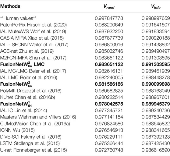
TABLE 2. Accuracy of various segmentation methods on the Drosophila EM dataset (ISBI 2012 EM segmentation challenge leaderboard, June 2020). Bold values correspond to the method presented here.

4.2 Zebrafish Data

The zebrafish EM data used here was taken from a publicly available database². It was captured from a 5.5 days post-fertilization larval specimen. This specimen was cut into ∼18,000 serial sections and collected onto a tape substrate with an automated tape-collecting ultramicrotome (ATUM) (Hayworth et al., 2014). A series of images spanning the anterior quarter of the larval zebrafish was acquired at $56.4\times 56.4\times \sim 60\mathrm{n}{\mathrm{m}}^3\mathrm{v}{\mathrm{x}}^{-1}$ resolution from 16,000 sections using scanning EM (Hildebrand, 2015; Hildebrand et al., 2017). All 2D images were then co-registered into a 3D volume using an FFT signal whitening approach (Wetzel et al., 2016). For training, two small sub-volume crops were extracted from a near-final iteration of the full volume alignment in order to avoid deploying later segmentation runs on training data. Two training volumes that contained different tissue features were chosen. One volume was 512 × 512 × 512 and the other was 512 × 512 × 256. The blob-like features of interest—neuronal nuclei—were manually segmented as area-lists in each training volume using the Fiji (Schindelin et al., 2012) TrakEM2 plug-in (Cardona et al., 2012). From each of these two training volumes, three quarters were used for training and one quarter was used for validation. These area-lists were exported as binary masks for use in the training procedure. For accuracy assessments, an additional non-overlapping 512 × 512 × 512 testing sub-volume and corresponding manual segmentation labels were used.

To assess the performance of $\mathrm{FusionNet}{\mathrm{W}}_{16}^4$ on this segmentation task, we first deployed it on 512 × 512 × 512 test volume alongside the U-net (Ronneberger et al., 2015) and RDN (Fakhry et al., 2017) methods. Figure 8 displays volume renderings of the zebrafish test set EM data, its manual cell nucleus segmentation, and segmentation results from U-net, RDN, and $\mathrm{FusionNet}{\mathrm{W}}_{16}^4$. As this shows, $\mathrm{FusionNet}{\mathrm{W}}_{16}^4$ introduced less false predictions compared to U-net and RDN. Table 3 compares U-net, RDN, and $\mathrm{FusionNet}{\mathrm{W}}_{16}^4$ using three quality metrics: foreground-restricted Rand scoring after border thinning (V_rand), foreground-restricted information theoretic scoring after border thinning (V_info), and the Dice coefficient (V_dice). By all of these metrics, $\mathrm{FusionNet}{\mathrm{W}}_{16}^4$ produced more accurate segmentation results.

FIGURE 8

FIGURE 8. Visual comparison of the larval zebrafish EM volume segmentation. (A) Input serial-section EM volume. (B) Manual segmentation (ground truth). (C) U-net (Ronneberger et al., 2015) result. (D) RDN (Fakhry et al., 2017) result. (E)$\mathrm{FusionNet}{\mathrm{W}}_{16}^4$ result. Red arrows indicate errors.

TABLE 3

TABLE 3. Segmentation accuracy on a test volume from the zebrafish EM dataset. Bold values correspond to the method presented here.

We also deployed the trained network to the complete set of 16,000 sections of the larval zebrafish brain imaged at $56.4\times 56.4\times \sim 60\mathrm{n}{\mathrm{m}}^3\mathrm{v}{\mathrm{x}}^{-1}$ resolution, which is about 1.2 terabytes in data size. Figure 9 shows EM dataset cross-sections in the transverse (top, x-y) and horizontal (bottom, x-z) planes of the larval zebrafish overlaid with the cell nucleus segmentation results. The transverse view overlay also shows the sphericity of each segmented cell nucleus in a blue to red color map, which can help to visually identify the location of false positives.

FIGURE 9

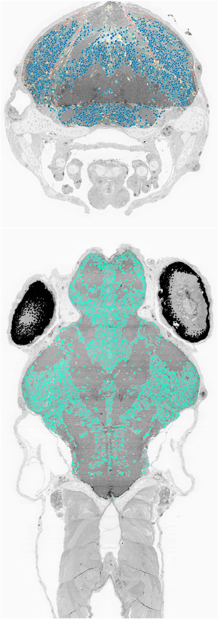
FIGURE 9. Cell nucleus segmentation results overlaid onto zebrafish EM volume cross-sections through the transverse (top, blue to red color map varies with cell sphericity) and horizontal (bottom) planes.

5 Conclusions

In this paper, we introduced a deep neural network architecture for image segmentation with a focus on connectomics EM image analysis. The proposed architecture, FusionNet, extends the U-net and residual CNN architectures to develop a deeper network for a more accurate end-to-end segmentation. We demonstrated the flexibility and performance of FusionNet in membrane- and blob-type EM segmentation tasks.

Several other approaches share similarities with FusionNet, particularly in concatenated chain forms. Chen et al. proposed concatenating multiple FCNs to build a RNN that extracts inter-slice contexts (Chen et al., 2016b). Unlike FusionNet, this approach takes as input multiple different resolutions of the raw image to produce a single segmentation output and uses a single loss function. Wu proposed iteratively applying a pixel-wise CNN (ICNN) to refine membrane detection probability maps (MDPM) (Wu, 2015). In this method, a regular CNN for generating MDPM from the raw input images and an iterative CNN for refining MDPM are trained independently. In contrast, FusionNet is trained as a single chained network. Additionally, FusionNet can refine errors in MDPM more completely using a chained network (i.e., by correcting errors in the error-corrected results) and scales better to larger image sizes due to the end-to-end nature of the network. More in-depth analyses into why chaining approaches are beneficial to improve the prediction accuracy of such deep networks will be an important goal for future work.

Data Availability Statement

The original contributions presented in the study are included in the article/Supplementary Material, further inquiries can be directed to the corresponding author.

Author Contributions

TMQ developed the methods and performed the experiments with input from W-KJ and DGCH. Project supervision and funding were provided by W-KJ. All authors wrote the paper.

Funding

This work was supported by a NAVER Fellowship to TMQ and by a Leon Levy Foundation Fellowship in Neuroscience to DGCH.

Conflict of Interest

The authors declare that the research was conducted in the absence of any commercial or financial relationships that could be construed as a potential conflict of interest.

Acknowledgments

We thank Woohyuk Choi and Jungmin Moon for assistance in creating the larval zebrafish EM volume renderings. This manuscript has been released as a pre-print at https://arxiv.org/abs/1612.05360 (Quan et al., 2016).

Footnotes

¹http://brainiac2.mit.edu/isbi_challenge/

²http://zebrafish.link/hildebrand16/

References

Arganda-Carreras, I., Turaga, S. C., Berger, D. R., Cireşan, D., Giusti, A., Gambardella, L. M., et al. (2015). Crowdsourcing the Creation of Image Segmentation Algorithms for Connectomics. Front. Neuroanat. 910, 142. doi:10.3389/fnana.2015.00142

PubMed Abstract | CrossRef Full Text | Google Scholar

Beier, T., Andres, B., Köthe, U., and Hamprecht, F. A. (2016). “An Efficient Fusion Move Algorithm for the Minimum Cost Lifted Multicut Problem,” in Proceedings of ECCV 2016, Amsterdam, Netherlands, October 8–16, 2016 (Springer, Cham), 715–730.

CrossRef Full Text | Google Scholar

Beier, T., Pape, C., Rahaman, N., Prange, T., Berg, S., Bock, D. D., et al. (2017). Multicut Brings Automated Neurite Segmentation Closer to Human Performance. Nat. Methods 14, 101–102. doi:10.1038/nmeth.4151

PubMed Abstract | CrossRef Full Text | Google Scholar

Bock, D. D., Lee, W.-C. A., Kerlin, A. M., Andermann, M. L., Hood, G., Wetzel, A. W., et al. (2011). Network Anatomy and In Vivo Physiology of Visual Cortical Neurons. Nature 471, 177–182. doi:10.1038/nature09802

PubMed Abstract | CrossRef Full Text | Google Scholar

Briggman, K. L., and Bock, D. D. (2012). Volume Electron Microscopy for Neuronal Circuit Reconstruction. Curr. Opin. Neurobiol. 22, 154–161. doi:10.1016/j.conb.2011.10.022

PubMed Abstract | CrossRef Full Text | Google Scholar

Briggman, K. L., Helmstaedter, M., and Denk, W. (2011). Wiring Specificity in the Direction-Selectivity Circuit of the Retina. Nature 471, 183–188. doi:10.1038/nature09818

PubMed Abstract | CrossRef Full Text | Google Scholar

Cardona, A., Saalfeld, S., Preibisch, S., Schmid, B., Cheng, A., Pulokas, J., et al. (2010). An Integrated Micro- and Macroarchitectural Analysis of the Drosophila Brain by Computer-Assisted Serial Section Electron Microscopy. PLoS Biol. 8 (10), e1000502. doi:10.1371/journal.pbio.1000502

PubMed Abstract | CrossRef Full Text | Google Scholar

Cardona, A., Saalfeld, S., Schindelin, J., Arganda-Carreras, I., Preibisch, S., Longair, M., et al. (2012). TrakEM2 Software for Neural Circuit Reconstruction. PLoS ONE 7 (6), e38011. doi:10.1371/journal.pone.0038011

PubMed Abstract | CrossRef Full Text | Google Scholar

Chen, H., Qi, X., Cheng, J., and Heng, P. (2016). “Deep Contextual Networks for Neuronal Structure Segmentation,” in Proceedings of the Thirtieth AAAI Conference on Artificial Intelligence, Phoenix, AZ, February 12–17, 2016 (AAAI Press), 1167–1173.

Google Scholar

Chen, J., Yang, L., Zhang, Y., Alber, M., and Chen, D. Z. (2016). “Combining Fully Convolutional and Recurrent Neural Networks for 3D Biomedical Image Segmentation,” in Proceedings of NIPS 2016, Barcelona, Spain, September 5, 2016 (Curran Associates, Inc.), 3036–3044.

Google Scholar

Chollet, F. (2015). Keras: Deep Learning Library for Theano and Tensorflow. Available at: http://keras.io/ (Accessed May 20, 2017).

Google Scholar

Cicek, O., Abdulkadir, A., Lienkamp, S. S., Brox, T., and Ronneberger, O. (2016). “3D U-Net: Learning Dense Volumetric Segmentation from Sparse Annotation,ˮ in Proceedings of MICCAI 2016, Athens, Greece, October 17–21, 2016 (Springer, Cham), 424–432.

CrossRef Full Text | Google Scholar

Ciresan, D., Giusti, A., Gambardella, L. M., and Schmidhuber, J. (2012). “Deep Neural Networks Segment Neuronal Membranes in Electron Microscopy Images,ˮ in Proceedings of NIPS 2012, Stateline, NV, December 3–8, 2012 (Curran Associates Inc.), 2843–2851.

Google Scholar

Drozdzal, M., Vorontsov, E., Chartrand, G., Kadoury, S., and Pal, C. (2016). “The Importance of Skip Connections in Biomedical Image Segmentation,ˮ in Proceedings of DLMIA 2016, Athens, Greece, October 21, 2016 (Springer, Cham), 179–187.

CrossRef Full Text | Google Scholar

Eberle, A. L., and Zeidler, D. (2018). Multi-Beam Scanning Electron Microscopy for High-Throughput Imaging in Connectomics Research. Front. Neuroanat. 12, 112. doi:10.3389/fnana.2018.00112

PubMed Abstract | CrossRef Full Text | Google Scholar

Ensafi, S., Lu, S., Kassim, A. A., and Tan, C. L. (2014). “3D Reconstruction of Neurons in Electron Microscopy Images,” in Proceedings of IEEE EMBS 2014, Chicago, Illinois, August 27–31, 2014 (IEEE), 6732–6735.

Google Scholar

Fakhry, A., Peng, H., and Ji, S. (2016). Deep Models for Brain EM Image Segmentation: Novel Insights and Improved Performance. Bioinformatics 32, 2352–2358. doi:10.1093/bioinformatics/btw165

PubMed Abstract | CrossRef Full Text | Google Scholar

Fakhry, A., Zeng, T., and Ji, S. (2017). Residual Deconvolutional Networks for Brain Electron Microscopy Image Segmentation. IEEE Trans. Med. Imaging 36, 447–456. doi:10.1109/tmi.2016.2613019

PubMed Abstract | CrossRef Full Text | Google Scholar

Gatys, L. A., Ecker, A. S., and Bethge, M. (2016). “Image Style Transfer Using Convolutional Neural Networks,ˮ in Proceedings of IEEE CVPR 2016, Las Vegas, NV, June 27–30, 2016 (IEEE), 2414–2423.

Google Scholar

Graham, B. J., Hildebrand, D. G. C., Kuan, A. T., Maniates-Selvin, J. T., Thomas, L. A., Shanny, B. L., et al. (2019). High-throughput Transmission Electron Microscopy With Automated Serial Sectioning. doi:10.1101/657346 Preprint. Available at: https://doi.org/10.1101/657346 (Accessed June 2, 2019).

CrossRef Full Text | Google Scholar

Hayworth, K. J., Morgan, J. L., Schalek, R., Berger, D. R., Hildebrand, D. G. C., and Lichtman, J. W. (2014). Imaging ATUM Ultrathin Section Libraries With WaferMapper: A Multi-Scale Approach to EM Reconstruction of Neural Circuits. Front. Neural Circuits 8, 68. doi:10.3389/fncir.2014.00068

PubMed Abstract | CrossRef Full Text | Google Scholar

He, K., Zhang, X., Ren, S., and Sun, J. (2016). “Deep Residual Learning for Image Recognition,ˮ in Conference on Computer Vision and Pattern Recognition (CVPR), Las Vegas, NV, June 27–30, 2016 (IEEE), 770–778.

Google Scholar

Helmstaedter, M. (2013). Cellular-Resolution Connectomics: Challenges of Dense Neural Circuit Reconstruction. Nat. Methods 10, 501–507. doi:10.1038/nmeth.2476

PubMed Abstract | CrossRef Full Text | Google Scholar

Hildebrand, D. G. C. (2015). Whole-Brain Functional and Structural Examination in Larval Zebrafish. PhD thesis. Cambridge (MA): Harvard University, Graduate School of Arts and Sciences.

Google Scholar

Hildebrand, D. G. C., Cicconet, M., Torres, R. M., Choi, W., Quan, T. M., Moon, J., et al. (2017). Whole-Brain Serial-Section Electron Microscopy in Larval Zebrafish. Nature 545, 345–349. doi:10.1038/nature22356

PubMed Abstract | CrossRef Full Text | Google Scholar

Hirsch, P., Mais, L., and Kainmueller, D. (2020). “Patchperpix for Instance Segmentation,” in Proceedings of ECCV 2020, Glasgow, United Kingdom, August 23–28, 2020 (Springer, Cham), 288–304.

CrossRef Full Text | Google Scholar

Isin, A., Direkoglu, C., and Sah, M. (2016). Review of MRI-Based Brain Tumor Image Segmentation Using Deep Learning Methods. Procedia Comput. Sci. 102, 317–324. doi:10.1016/j.procs.2016.09.407

CrossRef Full Text | Google Scholar

Jeong, W.-K., Beyer, J., Hadwiger, M., Blue, R., Law, C., Vázquez-Reina, A., et al. (2010). Secrett and NeuroTrace: Interactive Visualization and Analysis Tools for Large-Scale Neuroscience Data Sets. IEEE Comput. Graphics Appl. 30, 58–70. doi:10.1109/MCG.2010.56

PubMed Abstract | CrossRef Full Text | Google Scholar

Kaynig, V., Vazquez-Reina, A., Knowles-Barley, S., Roberts, M., Jones, T. R., Kasthuri, N., et al. (2015). Large-scale Automatic Reconstruction of Neuronal Processes From Electron Microscopy Images. Med. Image Anal. 22, 77–88. doi:10.1016/j.media.2015.02.001

PubMed Abstract | CrossRef Full Text | Google Scholar

Krizhevsky, A., Sutskever, I., and Hinton, G. E. (2012). “ImageNet Classification With Deep Convolutional Neural Networks, in Proceedings of NIPS 2012, Stateline, NV, December 3–8, 2012 (Curran Associates Inc.), 1097–1105.

Google Scholar

LeCun, Y., Bengio, Y., and Hinton, G. (2015). Deep Learning. Nature 521, 436–444. doi:10.1038/nature14539

PubMed Abstract | CrossRef Full Text | Google Scholar

Lee, G., Oh, J.-W., Kang, M.-S., Her, N.-G., Kim, M.-H., and Jeong, W.-K. (2018). “DeepHCS: Bright-Field to Fluorescence Microscopy Image Conversion Using Deep Learning for Label-Free High-Content Screening, ˮ in Medical Image Computing and Computer Assisted Intervention–MICCAI 2018, Granada, Spain, September 16–20, 2018 (Springer International Publishing), 335–343.

CrossRef Full Text | Google Scholar

Lichtman, J. W., and Denk, W. (2011). The Big and the Small: Challenges of Imaging the Brain’s Circuits. Science 334, 618–623. doi:10.1126/science.1209168

PubMed Abstract | CrossRef Full Text | Google Scholar

Lin, M., Chen, Q., and Yan, S. (2014). “Network in Network, ˮ in Proceedings of ICLR 2014. arXiv:1312.4400v3.

Google Scholar

Long, J., Shelhamer, E., and Darrell, T. (2015). “Fully Convolutional Networks for Semantic Segmentation,ˮ in Proceedings of IEEE CVPR 2015, Boston, MA, June 7–12, 2015 (IEEE), 3431–3440.

Google Scholar

Pape, C., Matskevych, A., Wolny, A., Hennies, J., Mizzon, G., Louveaux, M., et al. (2019). Leveraging Domain Knowledge to Improve Microscopy Image Segmentation with Lifted Multicuts. Front. Comput. Sci. 1, 657. doi:10.3389/fcomp.2019.00006

CrossRef Full Text | Google Scholar

Parag, T., Ciresan, D. C., and Giusti, A. (2015). “Efficient Classifier Training to Minimize False Merges in Electron Microscopy Segmentation,ˮ in Proceedings of IEEE ICCV 2015, Santiago, Chile, December 7–13, 2015 (IEEE), 657–665.

Google Scholar

Quan, T. M., Hildebrand, D. G. C., and Jeong, W.-K. (2016). FusionNet: A Deep Fully Residual Convolutional Neural Network for Image Segmentation in Connectomics. arXiv preprint arXiv:1612.05360.

Google Scholar

Quan, T. M., Nguyen-Duc, T., and Jeong, W.-K. (2018). Compressed Sensing MRI Reconstruction Using a Generative Adversarial Network With a Cyclic Loss. IEEE Trans. Med. Imaging 37, 1488–1497. doi:10.1109/tmi.2018.2820120

PubMed Abstract | CrossRef Full Text | Google Scholar

Ronneberger, O., Fischer, P., and Brox, T. (2015). “U-Net: Convolutional Networks for Biomedical Image Segmentation. ˮin Proceedings of MICCAI 2015, Munich, Germany, October 5–9, 2015 (Springer, Cham), 234–241.

CrossRef Full Text | Google Scholar

Russakovsky, O., Deng, J., Su, H., Krause, J., Satheesh, S., Ma, S., et al. (2015). ImageNet Large Scale Visual Recognition Challenge. Int. J. Comput. Vision 115, 211–252. doi:10.1007/s11263-015-0816-y

CrossRef Full Text | Google Scholar

Y. Shapira (Editor) (2008). Matrix-Based Multigrid. New York, NY: Springer US.

Schindelin, J., Arganda-Carreras, I., Frise, E., Kaynig, V., Longair, M., Pietzsch, T., et al. (2012). Fiji: an Open-Source Platform for Biological-Image Analysis. Nat. Methods 9, 676–682. doi:10.1038/nmeth.2019

PubMed Abstract | CrossRef Full Text | Google Scholar

Shen, W., Wang, B., Jiang, Y., Wang, Y., and Yuille, A. (2017). “Multi-stage Multi-Recursive-Input Fully Convolutional Networks for Neuronal Boundary Detection,ˮ in IEEE International Conference on Computer Vision (ICCV), Venice, Italy, October 22–29, 2017 (IEEE), 2391–2400.

Google Scholar

Simonyan, K., and Zisserman, A. (2014). Very Deep Convolutional Networks for Large-Scale Image Recognition. arXiv preprint arXiv:1409.1556

Google Scholar

Sommer, C., Strähle, C., Köthe, U., and Hamprecht, F. A. (2011). “Ilastik: Interactive Learning and Segmentation Toolkit,ˮ in Proceedings of IEEE ISBI 2011, Chicago, IL, March 30–April 2, 2011 (IEEE), 230–233.

Google Scholar

Stollenga, M. F., Byeon, W., Liwicki, M., and Schmidhuber, J. (2015). “Parallel Multi-Dimensional LSTM, with Application to Fast Biomedical Volumetric Image Segmentation,ˮ in Proceedings of NIPS 2015, June 24, 2015, Montreal, QC (Curran Associates, Inc.), 2998–3006.

Google Scholar

Szegedy, C., Liu, W., Jia, Y., Sermanet, P., Reed, S., Anguelov, D., et al. (2015). “Going Deeper with Convolutions,ˮ in Proceedings of IEEE CVPR, Boston, MA, June 7–12, 2015 (IEEE) 1–9.

Google Scholar

Turaga, S. C., Murray, J. F., Jain, V., Roth, F., Helmstaedter, M., Briggman, K., et al. (2010). Convolutional Networks can Learn to Generate Affinity Graphs for Image Segmentation. Neural Comput. 22, 511–538. doi:10.1162/neco.2009.10-08-881

PubMed Abstract | CrossRef Full Text | Google Scholar

Weiler, M., Hamprecht, F. A., and Storath, M. (2017). “Learning Steerable Filters for Rotation Equivariant cnns,ˮ in Computer Vision and Pattern Recognition, Honolulu, HI, July 21–26, 2017 (IEEE), 849–858.

Google Scholar

Wetzel, A. W., Bakal, J., Dittrich, M., Hildebrand, D. G. C., Morgan, J. L., and Lichtman, J. W. (2016). “Registering Large Volume Serial-Section Electron Microscopy Image Sets for Neural Circuit Reconstruction Using FFT Signal Whitening,ˮ in Proceedings of AIPR Workshop 2016, Washington, D.C., United States, October 18–20, 2016 (IEEE), 1–10.

Google Scholar

Wiehman, S., and Villiers, H. D. (2016). “Semantic Segmentation of Bioimages Using Convolutional Neural Networks,ˮ in Proceedings of IJCNN 2016, Vancouver, BC, July 24–29, 2016 (IEEE), 624–631.

Google Scholar

Wolf, S., Bailoni, A., Pape, C., Rahaman, N., Kreshuk, A., Köthe, U., et al. (2019). The Mutex Watershed and its Objective: Efficient, Parameter-Free Image Partitioning. IEEE Trans. Pattern Anal. Mach. Intell. doi:10.1109/TPAMI.2020.2980827

CrossRef Full Text | Google Scholar

Wu, X. (2015). An Iterative Convolutional Neural Network Algorithm Improves Electron Microscopy Image Segmentation. arXiv preprint arXiv:150605849.

Google Scholar

Xiao, C., Liu, J., Chen, X., Han, H., Shu, C., and Xie, Q. (2018). “Deep Contextual Residual Network for Electron Microscopy Image Segmentation in Connectomics,ˮ in IEEE 15th International Symposium On Biomedical Imaging (ISBI 2018), Washington, D.C., United States, April 4–7, 2018 (IEEE), 378–381.

Google Scholar

Zeiler, M. D., and Fergus, R. (2014). “Visualizing and Understanding Convolutional Networks,ˮ in Proceedings of ECCV 2014, Zurich, Switzerland, September 6–12, 2014 (Springer, Cham), 818–833.

CrossRef Full Text | Google Scholar

Zheng, Y., Liu, D., Georgescu, B., Nguyen, H., and Comaniciu, D. (2015). “3D Deep Learning for Efficient and Robust Landmark Detection in Volumetric Data,ˮ in Proceedings of MICCAI 2015, Munich, Germany, October 5–9, 2015 (Springer, Cham), 565–572.

CrossRef Full Text | Google Scholar

Zheng, Z., Lauritzen, J. S., Perlman, E., Robinson, C. G., Nichols, M., Milkie, D., et al. (2018). A Complete Electron Microscopy Volume of the Brain of Adult drosophila Melanogaster. Cell 174, 730–743. doi:10.1016/j.cell.2018.06.019e22

PubMed Abstract | CrossRef Full Text | Google Scholar

Zhu, Y., Torrens, Y., Chen, Z., Zhao, S., Xie, H., Guo, W., and Zhang, Y. (2019). “Ace-net: Biomedical Image Segmentation with Augmented Contracting and Expansive Paths,ˮin International Conference on Medical Image Computing and Computer-Assisted Intervention, Shenzhen, China, October 13–17, 2019 (Springer, Cham).712–720.

CrossRef Full Text | Google Scholar