Increasing Interpretability of Bayesian Probabilistic Programming Models Through Interactive Representations

Bayesian probabilistic modeling is supported by powerful computational tools like probabilistic programming and efficient Markov Chain Monte Carlo (MCMC) sampling. However, the results of Bayesian inference are challenging for users to interpret in tasks like decision-making under uncertainty or model refinement. Decision-makers need simultaneous insight into both the model's structure and its predictions, including uncertainty in inferred parameters. This enables better assessment of the risk overall possible outcomes compatible with observations and thus more informed decisions. To support this, we see a need for visualization tools that make probabilistic programs interpretable to reveal the interdependencies in probabilistic models and their inherent uncertainty. We propose the automatic transformation of Bayesian probabilistic models, expressed in a probabilistic programming language, into an interactive graphical representation of the model's structure at varying levels of granularity, with seamless integration of uncertainty visualization. This interactive graphical representation supports the exploration of the prior and posterior distribution of MCMC samples. The interpretability of Bayesian probabilistic programming models is enhanced through the interactive graphical representations, which provide human users with more informative, transparent, and explainable probabilistic models. We present a concrete implementation that translates probabilistic programs to interactive graphical representations and show illustrative examples for a variety of Bayesian probabilistic models.

1. Introduction

Bayesian probabilistic modeling has many advantages; it accounts for and represents uncertainty systematically; it allows precise incorporation of prior expert knowledge; and the intrinsic structure of models is well-defined in terms of relations among random variables: the mathematical and statistical dependencies are explicitly stated. Extremely flexible Bayesian probabilistic models can be implemented via Probabilistic Programming Languages (PPLs), which provide automatic inference via practical and efficient Markov Chain Monte Carlo (MCMC) sampling. However, tasks like decision-making under uncertainty or refinement of models require tools that could enable profound comprehension of model's structure and intuitive interpretation of Bayesian inference results.

A very simple probabilistic model with few parameters could allow a human decision-maker to contemplate the entire model at once and comprehend how parameters interact with each other and the predictions of the model. This becomes more challenging as the model becomes more complex, perhaps with hierarchical structure, multivariate distributions, complex inter-dependencies and increasingly abstract latent states. Mere understanding of model's parameters and their dependencies does not guarantee effective decision-making. Rational decisions should be based upon assessment of the risk of all possible states compatible with data; this is the key advantage of a Bayesian formulation. This requires authentic representation of the parameter uncertainty. We propose that it is essential to communicate the (conditional) uncertainty of the parameters alongside their dependency structure.

Communication of uncertainty has challenges. Bayesian reasoning is closely tied to reasoning about conditional probabilities. People with a weaker background in statistics can have difficulty reasoning about conditional probabilities (Tversky and Kahneman, 1974; Koller and Friedman, 2009). Some common difficulties are distinguishing conditional and joint probabilities, and the recognition that conditional probability involves a restriction in the sample space (Díaz and Inmaculada, 2007). But even in the cases that the decision-maker is fully aware of these issues in theory, it is practically difficult to reason about the conditional probabilities of a complex model.

Bayesian probabilistic modeling incorporates prior knowledge by defining probability distributions over a model's parameters based on knowledge before seeing data. These prior beliefs are transformed into posterior beliefs in the light of the observed data. We may also transform from a model's latent parameters space to observation space; if we do this before observing data we form the prior predictive distribution. After observing the data we form the posterior predictive distribution, which we may, for example, sample from to generate synthetic observations.

Bayesian statistics was largely confined to academic research since Thomas Bayes set the foundations in 1763 (Bayes and Price, 1763) until the late twentieth century, largely due to technical difficulties in inference and the specialized statistical knowledge required (Lambert, 2018). This started changing in the early 1990s with the appearance of practical Markov Chain Monte Carlo (MCMC) techniques (Spiegelhalter and Rice, 2009) and the emergence, some years later, of Probabilistic Programming Languages (PPLs). PPLs are used to concisely express a vast range of probabilistic models and offer efficient, well-tested algorithms for inference. PPLs hide technical details of inference from modelers, offering an integrated environment that automates inference once a model is specified.

There are visualization tools that seek to communicate inference results to users in a compact and relevant way, like ArviZ (Kumar et al., 2019), a unified library that provides tools for diagnostics and visualizations of Bayesian inference in Python. However, a complex Bayesian model could result in a high-dimensional posterior that would require unwieldy tables to present summary statistics or a multitude of visualizations that are difficult to grapple with. The more complex a Bayesian probabilistic model becomes, the more error-prone the specification process of a Bayesian probabilistic model becomes. We see a need for a tool that would automatically synthesize user interfaces to PPL inference results, creating a compact interactive graphical representation that would convey structural and inference-related information at varying granularity. This tool would replace large tables of statistics with interactive graphical representations which integrate the structural relation of parameters along with their inferred distributions. It would convey uncertainty accurately and support interactive sensitivity analysis.

This tool could support:

1. Decision-makers seeking to interpret inference results or make predictions;

2. Experts seeking to effectively express their prior beliefs and the implications of their beliefs on inference;

3. Data-scientists and statisticians seeking to refine and validate an inference process (debugging a PPL program such that it runs efficiently and correctly);

Therefore, in this work we propose a novel representation of Bayesian probabilistic models, the interactive probabilistic models explorer. The objectives are:

1. Automatic transformation of a PPL model into a graphical representation of the model's structure,

2. Seamless integration of uncertainty visualization into the graphical representation of the model,

3. Granularity in the presented visual information according to user's choices and needs,

4. Interactive exploration of inference MCMC sample space,

5. Inclusion of both prior and posterior beliefs, predictions and predictive checks.

The interactive probabilistic models explorer aims at increasing the informativeness of Bayesian probabilistic programming models by integrating uncertainty. It also enhances transparency of the model's structure by providing an at-a-glance representation of a PPL models' structure integrated with uncertainty representation. The transparency of the inference results is increased by the explorability introduced by the interactive elements.

The posterior (or prior) of a Bayesian probabilistic model is thought of as a high-dimensional entity. Users can interactively view different perspectives of this entity with low latency. These views could be thought of as projections of the posterior distribution. Through their explorations of the posterior, users can develop an intuitive understanding of the “fragility” of the model's uncertainty—in other words performing interactive sensitivity analysis—without having to explicitly reason about abstract conditional probabilities (Steegen et al., 2016). The interactive probabilistic models explorer offers an explorable explanation of the PPL model.

Finally, the proposed representation could enhance trust in the model by facilitating prior and posterior predictive checks that provide evidence for the model's consistency with the prior knowledge and the actual data generating processes. The interactive probabilistic models explorer could increase the interpretability of PPLs by providing more direct, visceral intuition about Bayesian reasoning, supplementing the abstract mathematical symbolic representation. As Bayesian probabilistic models increase penetration in science, research and industry, the demand for more interpretable Bayesian probabilistic models rises. This work aspires to provide a user interface to these models.

In section 2, we elaborate on the visual and functional objectives of the interactive probabilistic models explorer and present the main aspects of the design and implementation of a tool that we developed for the transformation of a PPL model into an interactive probabilistic models explorer. In section 3, we demonstrate illustrative examples of use. Finally, in section 4, we analyse the contributions of the proposed representation of probabilistic models and summarize our conclusions.

2. Method

2.1. Overview

Before we dive into the technical details of the design and development of the interactive probabilistic models explorer (IPME) tool, we elaborate the visual and functional objectives of the proposed representation. We then present the main aspects of the design and technical implementation of the IPME tool including some of the challenges that we had to face, and we discuss the limitations of the implementation.

2.2. Objectives of Interactive Probabilistic Models Explorer

The first objective of the interactive probabilistic models explorer is the transformation of a PPL model—some lines of code of a probabilistic programming language, potentially alongside some observed data—into a graphical representation of the model. We would like to be able to transform PPL models independently of the PPL and independently of the structure of the specific model implemented. By the term “graphical representation” we mean a coherent graph-like representation of the probabilistic model that would reveal the internal structure of dependencies among the model's parameters. By representing parameters as nodes and dependencies as directed edges, probabilistic models can be represented by directed acyclic graphs (DAGs) (Koller and Friedman, 2009) that visually capture the model's essence.

The second objective is the integration of the parameters' uncertainty into the graphical representation of the model. The prior and posterior distributions of a Bayesian probabilistic model are multi-dimensional joint distributions. The marginal distributions of the prior and posterior joint distributions of the model are slices, which reveal the uncertainty of a subset of (usually one of) the model's parameters. PPLs typically apply MCMC sampling to approximate prior and posterior distributions, and the marginal distribution that corresponds to each parameter of a model can easily be estimated from these samples. Figure 1A presents the posterior MCMC samples of a two-parameter model and Figure 1B shows the estimated 3D posterior distribution along with the 2D marginal distributions of the parameters (in dark blue). We could integrate the uncertainty of the model's parameters into the graphical representation of the model by including an uncertainty visualization (e.g., kernel density estimate, error bar, Box plot, CDF plot, dot quantile plot) of the parameter's estimated distribution into the node of the parameter.

FIGURE 1

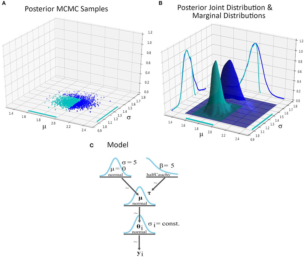
Figure 1. A two-parameter Bayesian model modeling the average minimum temperature in Scotland for the month November. The data provides the average minimum temperature in Scotland in month November for the years 1884–2020 and PyMC3 was used for the inference (see Supplementary Material for details). We explore the inference by setting two value range restrictions; μ ∈ [1.6, 2.0] and σ ∈ [1.0, 1.4]. (A) Posterior MCMC samples of the model's parameters. The samples that lie within the intersection of the value range restrictions are colored in cyan. (B) The estimated posterior distributions and marginal distributions based on the entire posterior MCMC sample set (dark blue) and the restricted sample set (cyan). (C) A DAG representation of the two-parameter Bayesian model as a Kruschke-style diagram (Kruschke, 2015). The posterior marginal distribution of μ (in cyan) in the subset of the posterior space became slightly tighter and shifted toward lower values of μ, which lead us to less uncertainty about expecting lower average temperature in Scotland for November given this particular conditioning.

The third objective of the interactive probabilistic models explorer is to provide adjustable granularity. Some users may wish to have a simplified summary view; while others may be involved in tasks like validating sampling and require detailed interactive visualizations. It would therefore make sense if the nodes of the model's graphical representation were collapsible in some way, and the user could interactively select the information that would be revealed to them.

The fourth objective is the interactive exploration of the model's uncertainty and ultimately, of the MCMC sample space. The exploration of the joint distribution would be important for providing answers to questions like the following ones:

1. What does the uncertainty of a parameter look like in a subset of the prior or posterior sample space based on the inference results of the model?

Answers to questions like this one could be crucial for decision-makers who would like to have estimates of a parameter's uncertainty under some specific conditions, which could, for example, represent a worst case scenario. This leads to some form of querying the results of an MCMC process; for example, a conjunctive restriction like 1.6 < μ <2.0 AND 1.0 < σ <1.4 for the mean and standard deviation of the average minimum temperature of the example in Figure 1. The sample space of the prior or posterior distribution can be restricted by setting bounds to the range of values of the individual parameters. Each restriction on the value range of a parameter defines a slice on the distribution. All the MCMC samples that belong to the subset of the restricted sample space define the uncertainty of the model within this subset of the sample space. In a conjunctive query, if we restrict the value range of more than one parameters, then the resulted subset of the sample space of the prior or posterior joint distribution is defined by the intersection of all the restricted value ranges of the parameters. For example, Figure 1A presents the MCMC samples that lie in the intersection of two value ranges restrictions in cyan and Figure 1B presents the re-estimated posterior distribution within the restricted sample space.

Such queries could be specified and reported visually if the user could interactively set value ranges and get the updated uncertainty visualizations for the entire model's joint distribution within the defined subset of the sample space. Such a query could be fed back to the sampler, so that a background sampling process could draw additional MCMC samples within the restricted sample space.

2. How sensitive is the uncertainty of a parameter to changes in the uncertainties of the rest of the parameters?

By restricting the value range of one or more parameters we can see the influence on the remaining parameters, because we only include the MCMC samples of the prior or posterior joint distribution that satisfy the constraints. We can therefore explore the sensitivity of parameters by observing how range restrictions on one parameter influence the uncertainty visualization of others. We could, for example, identify the parameters that are strongly coupled or, conversely, are wholly independent. This could be critical for decision-makers, who in the process of assessing the risk, would like to know how fragile the estimation of crucial parameters is.

The fifth objective is the inclusion of both prior and posterior parameter distributions, predictions and predictive checks. The Bayesian probabilistic models can provide estimations of the model's uncertainty both before and after seeing the observed data. In the first case, the estimations of the model for the uncertainty of the model and the predictions are based on the prior distributions. Exploring priors helps validate the realism of the prior beliefs once encoded in the PPL. Exploring posteriors reveals the results of the inference process following observations. Therefore we should include two visual representations in each node of the representation, one for the prior and one for the posterior distribution of the associated parameter.

The interactive probabilistic models explorer should also include prior and posterior predictions. A Bayesian model can simulate drawing samples in the space of observations, which is sometimes the ultimate task (e.g., in prediction), is sometimes essential for validation and calibration (e.g., in prior predictive checks) and is sometimes the most relevant way to explain consequences to users. The prediction of an observed variable's value by Bayesian probabilistic models is a distribution over possible (prior or posterior) observations (potentially approximated with samples, as in MCMC) and not just a single point estimate (see Supplementary Material for details about MCMC predictive sampling). This means that there is uncertainty about the predictions, which depends on the uncertainty of the rest of model's parameters. Nodes that represent observed variables should include an uncertainty visualization to present the predictions' uncertainty. This should be explored in conjunction with the distribution of the model's parameters; for example, any restriction on the prior or posterior sample space should propagate to the predictive distribution and vice versa.

2.3. Technical Implementation

In this section we will discuss the implementation of the tool we created for automatic transformation of a PPL model into interactive graphical representations. We will split our discussion into two parts. The first part will present the challenges of encoding any PPL model and associated inference results into a coherent structure. The second part will focus on the design and implementation of the interactive probabilistic models explorer itself.

2.3.1. PPL Model Encoding

One of the technical challenges that we had to overcome had to do with the ways that we could transform any PPL model into a graphical representation. We discriminate two types of information that the IPME tool will need; model-related information and inference-related information, and so we assume the input consists of:

• some transformation of the PPL source (i.e., the lines of code) that defines the model;

• the traces, the set of samples resulting from inference with an MCMC sampler; the output from “running” the model.

We restrict ourselves to MCMC approaches to inference in this paper, and so we always deal with collections of definite, (hopefully) independent samples representing possible model configurations. The traces can include samples from the prior, posterior, prior predictive and posterior predictive. We designed a pipeline to encode a PPL model and its inference results into a structure which is used as an input to the IPME tool. We defined steps that a modeler should take to export a PPL model and its inference results to the IPME tool. Figure 2 presents a diagrammatic representation of these steps. In this section, we will explain what these types of information should include and how their encoding is realized.

FIGURE 2

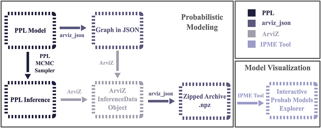
Figure 2. Flowchart showing the steps that a modeler should take to export the PPL-specified probabilistic model and the inference data into a standardized output, which will then be used as an input to the IPME module. The proposed pipeline adds three new steps to the typical model specification and inference running routine; the export of the PPL model graph into a JSON structure; the export of the inference data into an ArviZ InferenceData object, where we attach the structured description of the graph from the previous step; and finally, the export of all these into a collection of .npy arrays and metadata in a zipped file. We provide a concrete implementation of this pipeline through the arviz_json module, which was created for providing a standardized output for the PyMC3 models and inference data.

2.3.1.1. Model-related information

Model-related information is necessary for the construction of the graphical representation (DAG) of the model. The construction of a DAG requires, at minimum, the names of the nodes and their associations that define the edges. Therefore, the input of the IPME tool should include the model's variables names and a list of the parent nodes of each variable. We would also expect to be able to extract annotations for each parameter, including the distribution type (Gaussian, Poisson, binomial, Dirichlet etc.), data type (floating point, integer), tensor shape (uni-variate, N-d vector, MxN matrix, etc) and inferential type (observed, latent, deterministic).

A probabilistic model consists of either observed or unobserved variables. The observed variables are defined through a likelihood function and in a tree-like structure like a DAG, the lowest level of nodes consists of observed variables. The graph is “rooted” at the top with non-stochastic nodes with known, fixed values (e.g., constants used in specifying prior distributions). Unobserved variables could either be free parameters defined by prior distributions or they could be deterministic variables, transformations of other parameters; and it is also occasionally useful to define deterministic transformations of observed values. Thus, we define the inferential type of a probabilistic model's variable as one in the set {“observed”, “free”, “deterministic”}.

From our objectives, the interactive probabilistic models explorer should provide a collapsible view of the DAG. In the explorer, each node should provide some minimum information about the corresponding parameter. This could include the name of the parameter and the type of the parameter's distribution; this is sufficient to arrive at a graph similar to those of Kruschke (2015). The last model-related information needed is the dimensions and coordinates of the probabilistic model's variables; i.e., the tensor shape and its semantic structure. Parameters' dimensions usually correspond to dimensions of the observed data and they can be used to model groups of parameters. Interpreting tensor shapes in probabilistic programming is subtle (Ma, 2019) and may require additional annotation. The explorer depicts the uncertainty using 2D visualizations and allows the user to define the coordinates of the variables' dimensions.

We created a prototype structure that encodes the model-related information. The fields of this structure are defined by the model-related information that should be communicated as input to the IPME tool (see details about the JSON structure in the Supplementary Material). PPLs usually provide an API for allowing users to access this model-related information, though the provision and API to access this varies significantly. The modeler could access this information and produce the structure of the model's graph. For example, we have specifically developed a Python package called arviz_json¹ that provides an API for the transformation of PyMC3 (Salvatier et al., 2016) model objects into these structures.

2.3.1.2. Inference-related information and data

PPLs store inference results in different ways, which are usually backend-specific. For example, PyMC3 stores the MCMC samples in PyMC3 MultiTrace² objects, whereas PyStan stores inference results in PyStan StanFit objects. Thus, there is a need for a standardized backend-agnostic way of organizing and storing the inference-related information and results before forwarding it to the IPME tool. First of all, the MCMC samples that estimate the prior and posterior distributions of the unobserved variables of the model and the MCMC prior and posterior predictive samples for the observed variables of the model should be included to the tool's input. These samples should be stored in standardized structures and linked to the PPL model's variable names.

One solution to this problem is provided by the ArviZ library (Kumar et al., 2019), which provides an API for transforming the inference data of different inference back-ends and programming languages (PyMC3, PyStan, CmdStanPy, Pyro, NumPyro, emcee, and TensorFlow Probability objects) into ArviZ InferenceData³ data structures. The ArviZ InferenceData is a standardized data structure for inference results (MCMC samples) that is dependent on xarray's⁴ multi-dimensional array structures that introduce “labels in the form of dimensions, coordinates and attributes on top of raw NumPy-like multidimensional arrays.” InferenceData objects group various data sets that could be produced by a Bayesian analysis (prior or posterior samples, prior or posterior predictive samples, sample statistics etc.). ArviZ provides an API for exporting the InferenceData data structures in netcdf ⁵ files. Although our implementation of the interactive probabilistic models explorer was based on Python, we wanted to provide a generic solution that could work with any browser-based front end; we used the arviz_json package for exporting ArviZ InferenceData objects into a zip file containing JSON metadata with the model DAG and a collection of npy⁶ format arrays from the InferenceData object. There is also JSON metadata that link the model's variables to the data arrays and provide information about the type of the samples (prior, posterior), the dimensions and the coordinates (see details in the Supplementary Material).

2.3.2. Design and Implementation of the Explorer

We created a Python tool that takes as an input the output of the arviz_json module and creates the interactive graphical representation of the model. For the visualization we used Bokeh⁷, a Python interactive visualization library for modern web browsers, and Panel⁸, a Python library for interactive web apps and dashboards. The IPME tool provides a web-browser-based visualization of the interactive probabilistic models explorer and thanks to Bokeh that affords high-performance interactivity over large data sets, it provides a low-latency interactivity with the MCMC sample set.

The interactive probabilistic models explorer presents the model's DAG in a tree-like structure. We simplify the tree into rows of nodes ordered vertically from hyper-priors down to observed values. This format is a vertically ordered representation which orders nodes such that constant values (which are not shown) would be placed at the very top of the graphical representation and the lowest nodes in the graph are observed parameters. Parameter nodes are organized such that child nodes appear on rows lower than their parent prior distributions. In most hierarchical models, which have well-separated hyper-priors, this leads to a neat separation of the graph into rows and an obvious reading of the graph from top to bottom. There are, of course, graphs which are hard to arrange well in this format. Each node is a cell in a Panel GridSpec⁹ object. Each node of the graph has a toggle button, some text and a kernel density estimation (KDE) distribution plot. The toggle button is labeled by the variable's name, the tilde (~) symbol and the variable's distribution type, if the variable is observed or a free parameter, or the term “deterministic,” if the variable is deterministic. The text below the toggle button states the parent nodes and the dimensions of the parameter. The KDE curve can be hidden with the toggle button.

We present the uncertainty of parameters using a kernel density estimate¹⁰ (KDE), computed based on the corresponding MCMC samples, using Silverman bandwidth estimation. The KDE curve of the non-observed variables is estimated based on the MCMC samples of the (prior) posterior marginal distribution of the variable, while the KDE curve of the observed variables is estimated based on the (prior) posterior predictive MCMC samples. A rug plot is presented below the KDE curve to display the corresponding MCMC samples as ticks and give a better perception of the conditioning process on the sample space. We present two views of the DAG, one showing distribution in the nodes for the prior and one for the posterior space, in separate tabs so that users can both compare quickly.

The interactive probabilistic models explorer provides an interface for predictive model checking with predictive p-values. One way of checking the validity of a Bayesian model is by testing statistics of the observed data against the predictions of the model. The aspects of the observed data that are usually investigated could be defined as statistical metrics over the data. For example, the extreme observed values could be interpreted as the min and max value of the observations. Other common aspects of the data that could be checked are the mean and sd values.

A common metric for checking how well these statistics of the observed data are represented by the predictions of the model is the p-value; the probability Pr(metric_j(y_j) ≥ metric_j(obs)), where metric ∈ {“min”, “max”, “mean”, “sd”}, j ∈ {0, 1, .., N} and N is the size of the indexing dimension of the observed variable, y_j indicates the predictive samples of the model for the j coordinate of the indexing dimension, and obs the actual observed data (Sinharay and Stern, 2003). The prior and posterior histograms of these four statistical metrics over the posterior predictive samples are presented in two extra separate tabs. The actual observed value of each test statistics is indicated by a vertical black line on the corresponding histogram. The (Bayesian) p-values are also noted on the x-axis labels.

The IPME tool uses the dimensions and coordinates information to automatically create a widget box on the left-side of the graphical representation. Each indexing dimension of the model is converted into a drop-down menu or a slider presenting to the users the semantically meaningful coordinates of the indexing dimensions and allow them to change their values and get a different view of the data. The user can perform interactive sub-setting of any parameter by drawing a variable-width selection box to define a value range for the specific parameter. The part of the KDE curve that is enclosed into the selection box is highlighted and a second KDE curve that is computed based on the restricted MCMC sample set is drawn in a different color. The rug plot is updated accordingly. The color palette of the “arviz-darkgrid” style was used because it was designed to be color-blind friendly and it would add a tone of familiarity for the users of the ArviZ library. The user can update their initial selection by drawing a new selection box or can draw additional selection boxes on other distributions to add constraints to the query.

Every time the user draws a selection box, both the prior and the posterior spaces are restricted to include only samples that lay within the selected subset. The user can restrict the value range of any parameter at any coordinate of any indexing dimension and the restriction to the sample space will be reflected in both the prior and posterior, as well as to the prior and posterior predictive histograms. This kind of interaction allows the user compare the changes in the uncertainty in the restricted space between the prior and posterior beliefs about the model parameters. The user can also remove the restriction of a parameter by clicking on the “x” button that accompanies the updated KDE. Finally, the user can reset all the uncertainty visualizations by globally removing all the restrictions by pressing a “Global Reset” button.

2.4. Limitations of the Implementation

In this section, we will discuss the limitations of the IPME tool implementation. First of all, feeding back re-specified prior distributions and rerunning the inference is something that would be useful, but requires additional engineering to implement the feedback path to the sampler. For this reason, there might be cases where restrictions on the sample space exhaust the available samples and result in very small or empty sample sets. The IPME tool currently does not handle these cases well. We currently only support a single restriction in value range per parameter.

There are two issues connected to the presentation of the tree-like structure of the graph and the KDEs that we came across during the implementation of the tool. First, because a tree level with many nodes is not uncommon, we have to limit the number of nodes in each row to avoid horizontal scrolling. If a tree level has more than some maximum number of nodes, we break the row into two or more rows. Because this presentation spoils the tree-like feeling of the structure, we left-aligned the rows that correspond to the same level of the tree to give the feeling of the continuation for these rows. This is analogous to typesetting text: nodes are words, which are broken at the end of lines for visual presentation, and separated into paragraphs which are semantically distinct levels, offset with vertical spacing and indentation.

The second presentation issue had to do with the scaling of the KDEs. We did not apply any normalization to the KDEs so that we present the prior and posterior distributions as valid probability distributions, namely the area under the KDE graph sums to 1. If we apply normalization, this would obscure changes in the uncertainty in the subsets of the MCMC sample set. However, this lack of normalization could lead to significant differences in the maximum a posteriori (MAP) estimation¹¹ of the initial and updated KDE in cases of restricting the sample space to highly dense subsets. In these cases the overlap of the KDEs retaining their scales will present a very tiny initial KDE in comparison to the updated one and the user might need to use the “zoom wheel” tool to inspect the initial KDE.

3. Results

3.1. Presentation of the Probabilistic Programming Model's Graph

In this section, we discuss how other PPL-linked available tools display the graph structure of probabilistic models and compare this with the IPME tool. Figure 3B presents the probabilistic graphical model of the centered hierarchical model of the eight schools problem (see Supplementary Material) created with DoodleBUGS¹². Figure 3C presents the probabilistic graphical model of the same model using the PyMC3 Graphviz interface¹³. Although both ways present the structure of the probabilistic model as a graph providing an at-a-glance representation of the model's parameters and dependencies derived from the PPL specification of the model, they both lack the presentation of the parameters' uncertainty. Figure 3D presents (a manually created) Kruschke-style diagram of the same model, which is more informed since it presents the prototypes of the prior distributions of the model's parameters. But still, this latter representation of the probabilistic model does not give us any indication of the actual distributions of latent parameters.

FIGURE 3

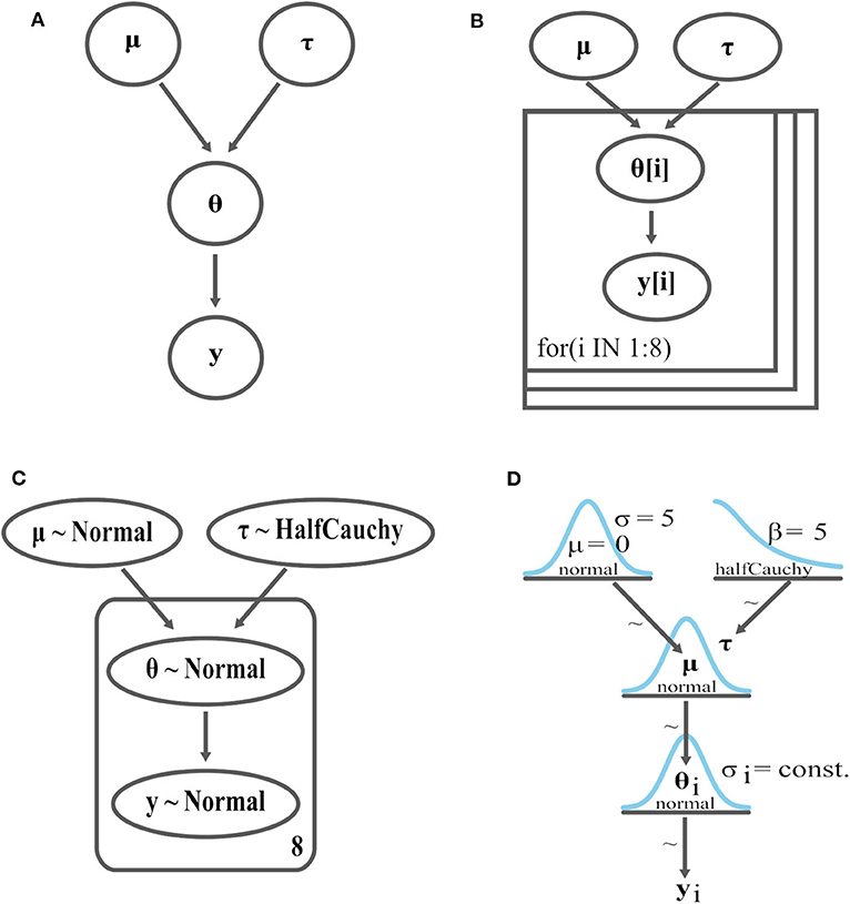
Figure 3. Graphical representations of the eight schools model, (A) Bayesian network, (B) DoodleBUGs graph, (C) PyMC3 graph using the Graphviz interface, (D) Kruschke-style diagram. These representations do not include estimations of the parameters' posterior uncertainty based on the simulation of real-data (i.e., MCMC samples).

Using the framework presented in Figure 2, we created the interactive probabilistic models explorer of the centered hierarchical model of the eight schools problem. Figures 4A,B presents the interactive probabilistic models explorer for the prior and posterior space, respectively, as an expanded DAG and Figure 4C presents its collapsed form. The interactive probabilistic models explorer seamlessly integrates the actual uncertainty estimations into the graph's nodes and provides variable granularity by allowing users to collapse certain elements. The widget box on the left-hand side contains one widget per indexing dimension and allows selecting different views of the inference data. Finally, the top tab switches between prior and posterior.

FIGURE 4

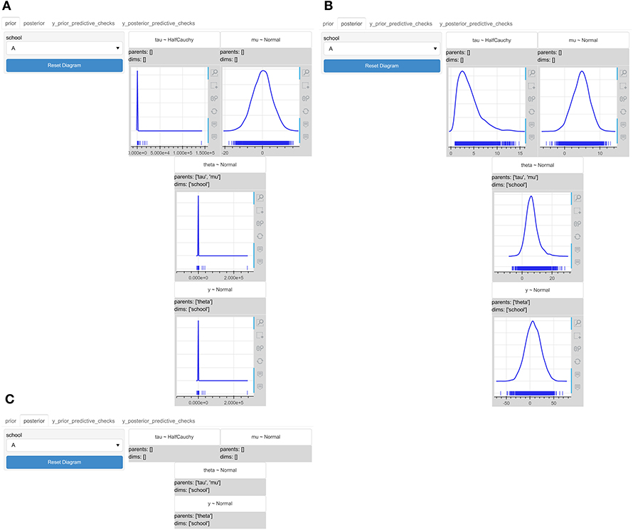
Figure 4. The interactive probabilistic models explorer of the centered hierarchical model of the eight schools problem. PyMC3 was used for the model's specification and inference. (A) The prior graphical representation. (B) The posterior graphical representation. (C) The collapsed graphical representation. The interactive probabilistic models explorer integrates the simulated inference data and provides variable granularity in the amount of the presented information.

3.2. Presentation of the Inference Results

In this section we compare the way that inference results are presented using typical presentation practices with the way the IPME achieves this, and discuss how the IPME was designed to provide a more compact and flexible presentation of the inference data. The most common practice in the reporting of inference results in Bayesian analysis is tables that present summary statistics of the posterior distributions. As model parameters or coordinates of indexing dimensions increase, these tables become unwieldy. For example, Silva et al. (2015) use a rather massive table of summary statistics when analyzing data of wildfires in Portugal between 1990 and 1994. The limited capacity of human cognition could be a hurdle for users like decision-makers to grasp the uncertainty presented in tables of this sort and assess the risk appropriately. The numerical data presented are usually statistics like mean, standard deviation or confidence intervals, which could mislead or overwhelm unfamiliar users.

A static representation of the inference data in summary tables cannot communicate sensitivity of the parameters, which would allow decision-makers to assess the impact of parameter inter-dependencies and associated risks. Communicating the prior would imply communicating a second table of similar complexity, which is often omitted in reports of Bayesian probabilistic models. For example, Table 1 presents the summary statistics of the posterior of the centered hierarchical model for the eight schools problem. We used the ArviZ API (arviz.summary) to produce this table.

TABLE 1

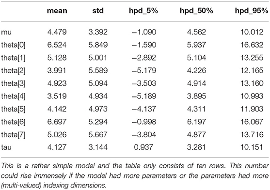
Table 1. Posterior statistics in a tabular format for the centered hierarchical model of the eight schools problem.

Another way of communicating inference results is by generating an uncertainty visualization for each model's parameter independently. This solution is not very common, although it is more informative than the tables of summary statistics. The reason is that it leads to a high number of visualizations in the case of many-parameter models, which are difficult to communicate in a concise way. For example, Figure 5 presents the posterior densities for the parameters of the centered hierarchical model of the eight schools problem. Although, this is a rather simple model, we can see that it can produce ten different uncertainty visualizations. This number could rise even more if the parameters of the model had more indexing dimensions or the indexing dimensions had more coordinates.

FIGURE 5

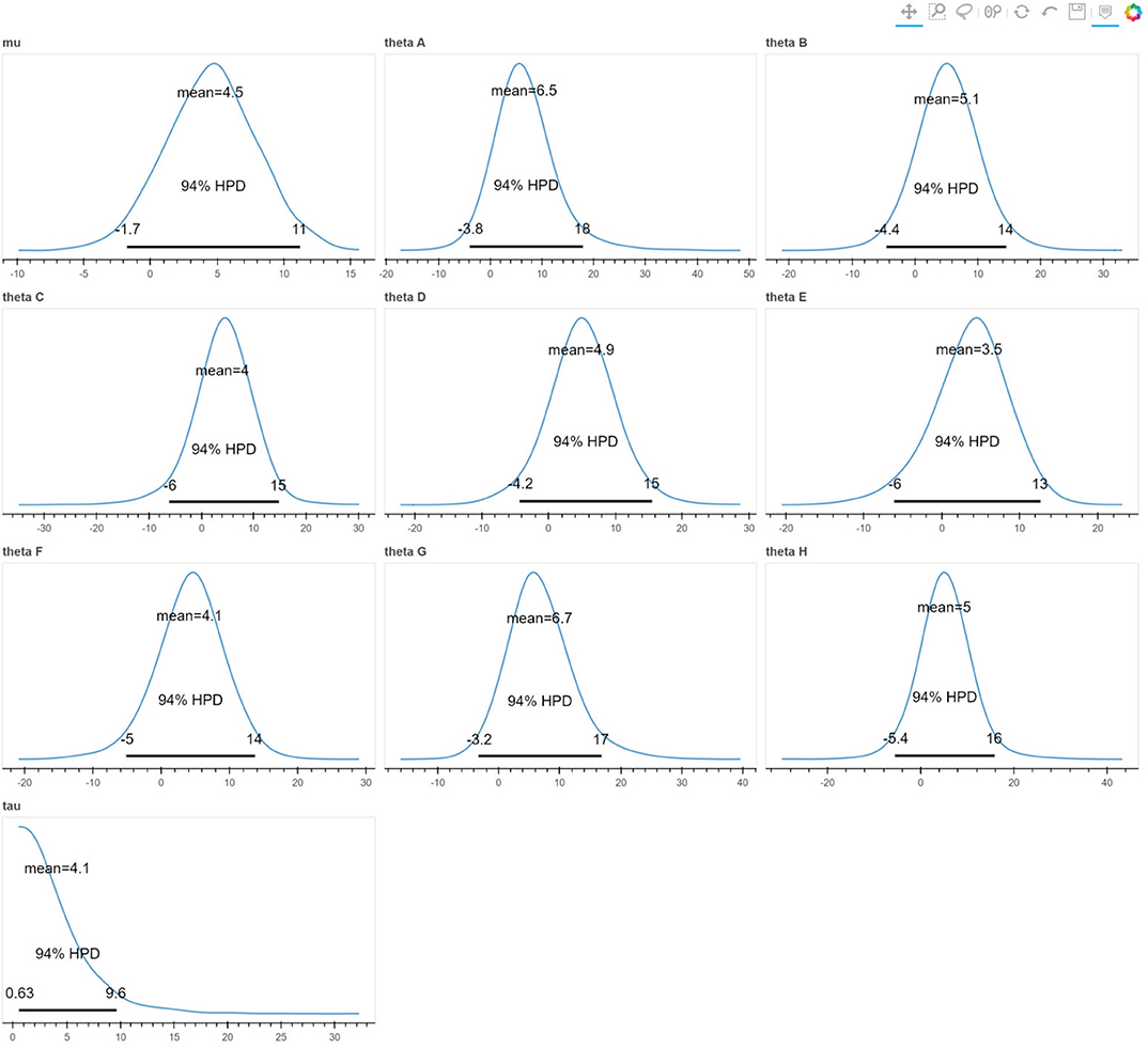
Figure 5. The posterior densities of the centered hierarchical model of the eight schools problem presented in the style introduced by Kruschke (2015). Although, this is a rather simple model, we can see that it can produce ten different uncertainty visualizations. This number could rise even more if the parameters of the model had more (multi-valued) indexing dimensions.

The IPME tool presents a summary presentation of the model's parameters in two similar tree-like structures (prior, posterior) that are as big as the number of the models parameters. The number of the indexing dimensions or coordinates does not affect the size of the graphical representations, in comparison with the summary statistics tables or uncertainty visualizations approach where each extra coordinate results in an extra row in the table or an extra visualization. The presentation of inference results with the IPME tool becomes more compact and concise. Users have more flexibility in the exploration of inference results with IPME; they can define the coordinates of the indexing dimensions, expand the nodes of interest and collapse the rest, compare priors to posteriors.

3.3. Use Case Scenarios

In this section, we present use case scenarios, where IPME is used to deal with a realistic modeling problem. The IPME tool could assist modelers in model checking and validation. The IPME provides two possibilities for checking the model. The first arises through the prior interactive graphical representation, where users could explore and observe the prior beliefs that were set during the model definition process and the prior predictive distributions along the various coordinates of the indexing dimensions. The consistency of the model's priors with the prior knowledge and experience could be investigated in this way. The second arises from the prior and posterior predictive model checking with predictive p-values. Users could observe how well aspects of the observed data are represented in the predictions of the model.

The IPME tool could also help users acquire a more intuitive comprehension of various aspects of the model and the inference results. This could be achieved through the interactivity. The IPME offers two types of interactivity; the interaction with the indexing dimensions that allows the exploration of the data from different viewpoints, and the interactive conditioning on the sample space that allows the exploration of the prior and posterior sample spaces. The first type of interactivity could reveal similarities or differences between groups of data. The second type of interactivity could reveal associations between parameters, changes in the parameters and predictions uncertainty under certain circumstances (conditions), or the effects of priors on posteriors. The following use case scenarios illustrate the ways that IPME could deal with realistic modeling problems.

3.3.1. Drivers Reaction Times

A common task in the working routine of a logistics company is the allocation of routes to drivers. A logistics company wants to optimize the allocation process by minimizing the risk of accidents when allocating long routes to drivers that are susceptible to tiredness under sleep-deprivation conditions. The data scientist of the company retrieved from the company's database the reaction times of the drivers in 10 consecutive days of driving under sleep-deprivation conditions, and fitted a pooled and a hierarchical linear regression model to predict the reaction times of the drivers on each day of driving (see more details in Supplementary Material). The bigger the slope of the regression line is, the more tired (bigger reaction times) the drivers get after consecutive days of driving.

3.3.1.1. Model check

The data scientist first used the IPME to check the models. The models were both predicting a priori negative slopes (Figure 6) meaning that drivers could have faster reaction times as days were passing by. That was not very realistic, but could happen with a small probability. The models were also predicting negative reaction times meaning that drivers could react before even they see a stimulation. Very big reaction times, close to tens of seconds, were also predicted as were moving closer to the 10th day. It seems that the priors might need to be updated. The data scientist was wondering which model of the two is the most appropriate one to trust, and thus, observed the posterior predictive test statistics of both models. Figures 7A,B present the four histograms for the pooled and hierarchical model, respectively. If none of the p-values of the test statistics is too high or low, the model is considered to generate “replicate data” similar to actual observed one based on the criteria of the provided test statistics. For example, the pooled model gives a very low posterior p-value for the “min” test statistics, which is improved in the hierarchical model. The hierarchical model improves the p-values of the “min,” “max,” and “std” test statistics of the observations in the predictions.

FIGURE 6

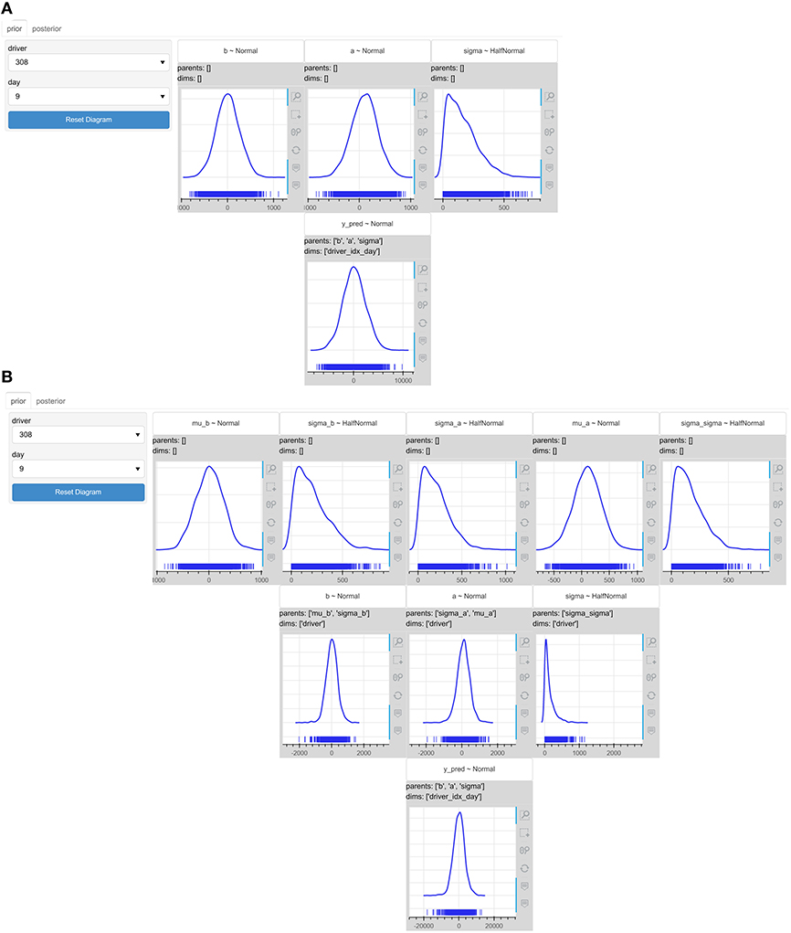
Figure 6. The interactive probabilistic models explorer of the reaction times models. PyMC3 was used for the models' specification and inference. (A) The prior graphical representation of the pooled model. (B) The prior graphical representation of the hierarchical model. The models predict negative slopes, and negative or very big (tens of seconds) values of reaction times a priori, which indicate that the priors might need to be updated.

FIGURE 7

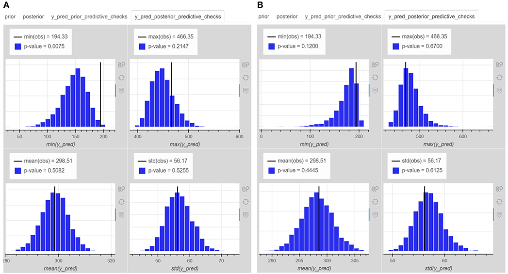
Figure 7. The posterior predictive test statistics of (A) the pooled reaction times model, (B) the hierarchical reaction times model. The hierarchical model improves representation of the “min” “max”, and “std” test statistics of the observations in the predictions.

3.3.1.2. Interactivity

Using the interactive drop-down menus, the data scientist observed the posterior predictive distribution of each driver on the same day of driving and realized that the pooled model did not present significant differences in the uncertainty of the predicted reaction times among drivers in contrast to the hierarchical one, which actually did (Figure 8). The data scientist kept the hierarchical model and passed it over to the logistics manager.

FIGURE 8

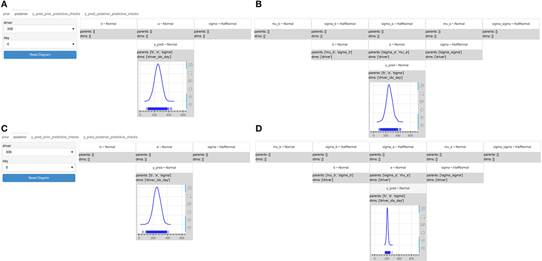
Figure 8. The interactive probabilistic models explorer of the reaction times models, where we set the driver to 308 and 309 and observe the posterior predictive distribution of the reaction times on the same day of driving for the pooled and hierarchical model. The posterior predictive distribution of the reaction times (A) for driver 308 in the pooled model, (B) for driver 308 in the hierarchical mode, (C) for driver 309 in the pooled mode, and (D) for diver 309 in the hierarchical model. The pooled model does not reveal significant differences among drivers.

The logistics manager had to choose between two available drivers, driver 310 and 335, who would take over an urgent shipping of a cargo that had to be delivered in 6 days, although it would normally require 9. Using the drivers drop-down menu, the logistics manager observes the uncertainty of the predicted reaction times for both drivers on the 6th day of driving (Figure 9); driver 310 has a wider distribution (more uncertainty), but centered to lower reaction times, whereas driver 335 has a tighter distribution (less uncertainty), but centered to higher reaction times.

FIGURE 9

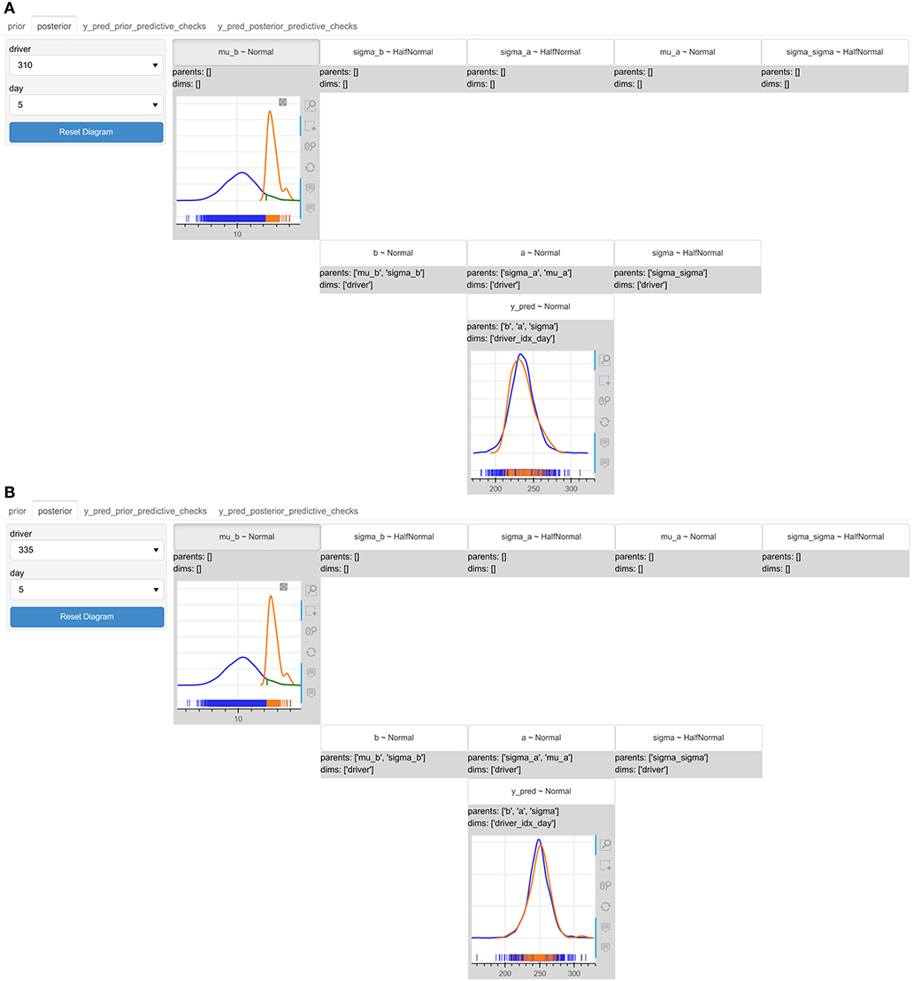
Figure 9. The interactive probabilistic models explorer of the reaction times hierarchical model. We compare drivers 310 and 335 and observe the posterior predictive distribution of the reaction times on day 6 (indexed by 5) setting a condition mu_b > 12.1. (A) The initial (in blue) and re-estimated (in orange) posterior predictive distribution of the reaction times for driver 310 on day 6. (B) The initial (in blue) and re-estimated (in orange) posterior predictive distribution of the reaction times for driver 335 on day 6. Driver 310 seems more robust to a possible worst case of high slopes predictions.

The logistics manager would like to see how the uncertainty of the predicted reaction times would look like in the worst case of the model's predictions; the bigger values of slope. He sets a condition on the hyper-prior of the mean value of the slopes to restrict the posterior sampling space to higher values of slopes. The distribution of driver 310 becomes wider with a slight shift to lower reaction times, whereas the distribution of driver 335 becomes again wider with a slight shift to higher reaction times. It seems that driver 310 is more robust to the worst case conditioning, although initially he was having more uncertainty over his predictions in comparison to driver 335.

3.3.2. Stochastic Volatility

There are periods of time when assets' returns are highly variable, which implies greater uncertainty about the actual values of the returns of the assets the next day. The day returns of assets is defined as the difference in asset's price at the end of the day in comparison to the start of the day over the initial asset price at the start of the day, R_t = (P_t − P_t−1)/P_t−1. The models that are used to predict the assets' returns use a latent volatility variable, volatility. The following probabilistic statements relate the returns variable to the volatility parameter based on the specification of such a model (see more details in Supplementary Material):

$\begin{array}{ll}\nu ~\text{Exp}(\lambda =0.1)& (1)\end{array}$

$\begin{array}{ll}\text{volatility }~\text{ GaussianRandomWalk}(\sigma =\text{step}\_\text{size})& (2)\end{array}$

$\begin{array}{ll}\text{returns }~\text{ StudentT}(\nu =\nu ,\lambda =\text{exp}(-2*\text{volatility}))& (3)\end{array}$

3.3.2.1. Model check

Looking at the prior predictive distribution of the returns variable in Figure 10, we realize that the model produces extremely large values of prior predictive returns, which are not reasonable, especially if we think that “the total value of all goods and services the world produces is $10⁹”¹⁴. We might need to change our prior distributions because they seem to fail to capture the prior knowledge well.

FIGURE 10

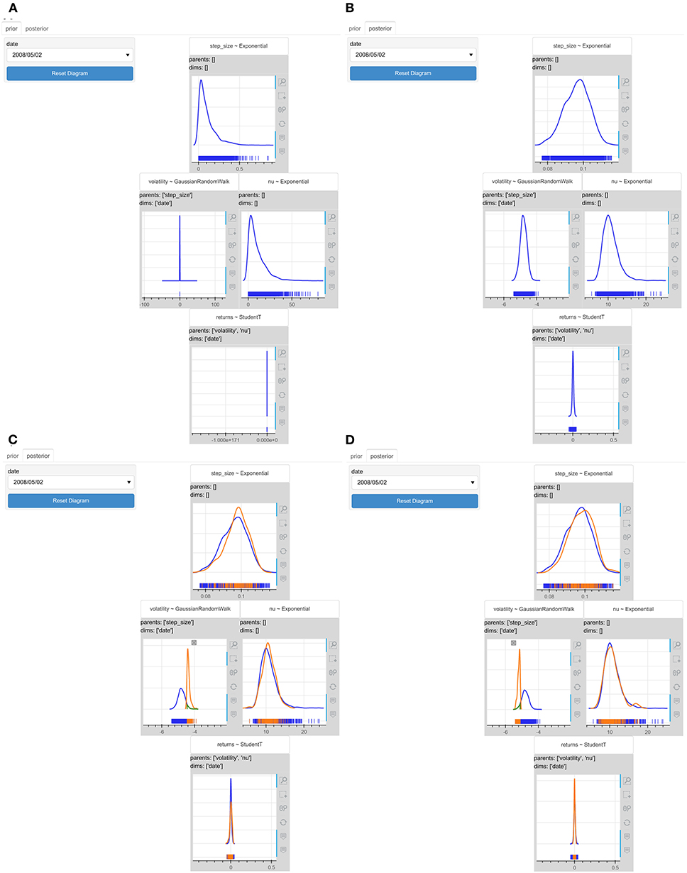
Figure 10. The interactive probabilistic models explorer of the stochastic volatility model. PyMC3 was used for the models' specification and inference. (A) The prior graphical representation. (B) The posterior graphical representation. (C) The updated posterior graphical representation after restricting the volatility to values greater than −4.5. (D) The updated posterior graphical representation after restricting the volatility to values smaller than −5.1. The greater the value of the volatility, the more uncertain the model becomes about the predicted values of the returns.

3.3.2.2. Interactivity

It is difficult to explain how volatility affects the predictive distribution of returns based solely on the model specification. To reason about this, users would need to be familiar with the λ parameter of the StudentT distribution and with the exponential transformation. The IPME could help into this as Figures 10C,D illustrate. When we restrict the volatility to values higher than −4.5 (Figure 10C), the predictive distribution of the returns variable becomes wider and therefore, the model becomes more uncertain about the values of the returns. On the other hand, when we restrict the volatility to values lower than −5.1 (Figure 10D), the predictive distribution of the returns variable becomes tighter and the model becomes less uncertain about the values of the returns.

In this example we could also use interaction to observe the effect of priors informativeness into the posteriors. The model uses a quite wide exponential distribution (with λ = 0.1) as a prior for the degrees of freedom parameter (ν) of the StudentT distribution. We could set a condition on the prior distribution of (ν) to make it tighter and see how the posteriors will change. We restrict ν ∈ [21.0, 30.0] in Figure 11A. The posterior distribution of volatility and the posterior predictive distribution of returns on day “02/05/2008” become tighter in Figure 11B. It is obvious that the more informative a prior is, the less uncertainty the model gives to its predictions.

FIGURE 11

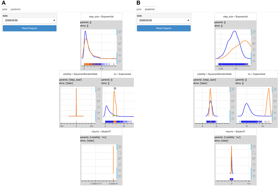
Figure 11. The interactive probabilistic models explorer of the stochastic volatility model where we set the condition ν ∈ [21.0, 30.0]. (A) The prior graphical representation. (B) The posterior graphical representation. The posterior distribution of volatility and the posterior predictive distribution of returns become tighter. More informative priors make model be more certain about its predictions.

3.3.3. Coal Mining Disasters

The coal mining disasters model (see more details in Supplementary Material) models the recorded coal mining disasters in the UK from 1851 to 1962 (Figure 12). During this period changes in the safety regulations are thought to have influenced the frequency of disasters. Thus, the model tries to predict a switch-point, when the disasters seemed to start declining. According to the probabilistic model presented in Figure 12B, the posterior probability mass function of the switchpoint variable indicates that the switch most probably took place at some point around the year 1890.

FIGURE 12

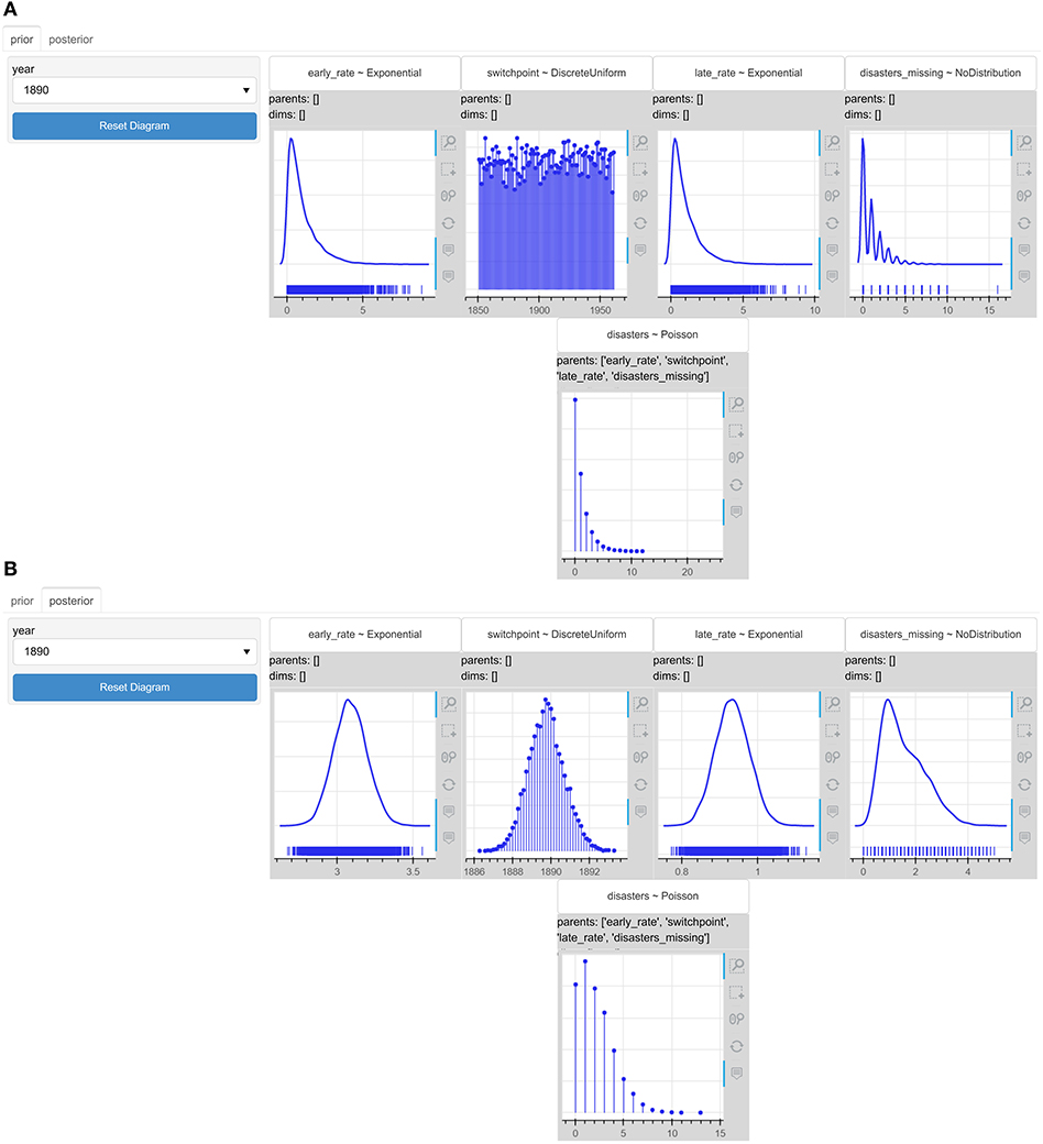
Figure 12. The interactive probabilistic models explorer of the coal mining disasters model. PyMC3 was used for the models' specification and inference. (A) The prior graphical representation. (B) The posterior graphical representation.

3.3.3.1. Interactivity

We could select the year 1890 from the year drop-down menu so that we can observe the uncertainty of the posterior predictions about the number of disasters in this year. Most of the probability mass is concentrated around the values of 1 or 2 disasters. What would happen to the uncertainty of the model about the number of disasters in year 1890 if the switch happened between 1893 and 1897?

Figure 13A presents how the uncertainty about the disaster number changes a priori based on the this condition on the switchpoint variable. The prior predictive probability mass function of the disasters variable becomes more dispersed, but the model does not seem to believe that the number of the disasters in year 1890 could be increased given the change in the regulations happens after 1890. Figure 13B shows the posterior predictive probability mass function of disasters becomes more dispersed and the probability mass gets slightly shifted toward 4. The model becomes more uncertain about the number of disasters and the mean increases slightly. This is reasonable, because if regulations changed after 1890, the number of disasters in year 1890 is expected to be increased.

FIGURE 13

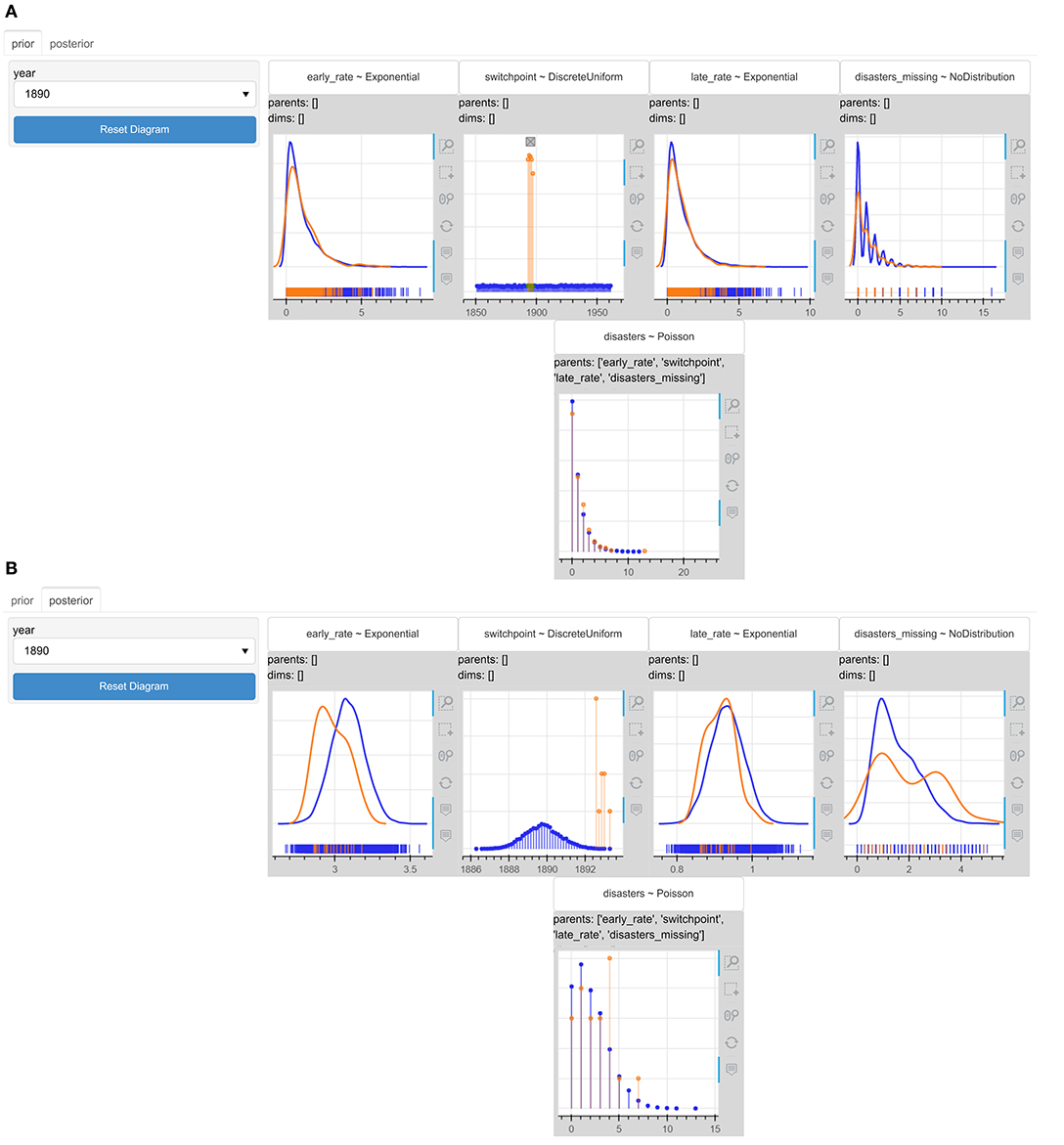
Figure 13. The interactive probabilistic models explorer of the coal mining disasters model. PyMC3 was used for the models' specification and inference. The updated (A) prior graphical representation, and (B) posterior graphical representation after restricting the switchpoint to values within the interval 1893−1897. The posterior predictive probability mass function of the number of disasters in year 1890 shifts toward 4. This is reasonable as we assumed with our conditioning that the regulations changed at a later time.

4. Discussion

4.1. Related Work

4.1.1. Probabilistic Graphical Models

One common representation of probabilistic models is Bayesian networks (Koller and Friedman, 2009). Bayesian networks model conditional dependencies among random variables, represented as nodes with conditional dependencies represented as edges in a directed acyclic graph (DAG). For example, the edge (μ, θ) that connects nodes μ and θ and is directed from μ to θ in Figure 3A expresses the conditional probability P(θ|μ) in the centered hierarchical model of the eight schools problem. Bayesian networks satisfy the local Markov property, which states that a node is conditionally independent of its non-descendants given its parents. For example, the conditional probability of node y given its parent node θ is conditionally independent of nodes μ and τ:

$\begin{array}{ll}P(y|\theta ,\mu ,\tau )=P(y|\theta ).& (4)\end{array}$

A posterior distribution can be expressed as a product of conditional probabilities based on the chain rule of probability:

$\begin{array}{l}P(y,\theta ,\mu ,\tau )=P(y|\theta ,\mu ,\tau )·P(\theta |\mu ,\tau )·P(\mu |\tau )·P(\tau )\\ =P(y|\theta )·P(\theta |\mu ,\tau )·P(\mu )·P(\tau )& (5)\end{array}$

From equation 5 we can see how Bayesian networks provide a factorized representation of joint probability distributions, where each edge expresses one factor in the joint probability.

PPLs do not usually provide tools or interfaces for automatic transformation of a probabilistic programming model into a DAG. Two PPLs that provide some form of graphical model interchange are BUGS (via DoodleBUGS) and PyMC3. DoodleBUGS is a software component of WinBUGs (Spiegelhalter et al., 2003) that provides a Doodle editor for creating probabilistic graphical models as DAGs and automatically transcribing DAGs into BUGs language (Lunn et al., 2009). However it cannot do the opposite, namely transform a model written in BUGS into a DAG. Figure 3B presents the graphical probabilistic model of the eight schools' hierarchical model that was created with DoodleBUGs. PyMC3 (Salvatier et al., 2016) provides the pymc3.model_graph.model_to_graphviz(model =None) method that converts a PyMC3 model into a graphviz Digraph using the Graphviz graph visualization software (Ellson et al., 2004). Figure 3C presents the graphical model of the PyMC3 eight schools' model.

Kruschke (2015) introduced a more informative DAG that shows iconic “prototypes” of the distributions on each node of the diagram. Kruschke (2012) argues that this type of diagram (in comparison to the ones created with DoodleBUGS) has “a much more direct correspondence to lines of code in JAGS/BUGS: (Usually) each arrow in this diagram corresponds to a line of code in the JAGS/BUGS model specification.” Kruschke (2012) explains that this type of diagram indicates which parameters participate in the same distribution, which is not visible in DoodleBUGs graphs. There is no automatic tool for the creation of this Kruschke-style diagram, but Kruschke (2013) presents two drawing tools that were created specifically for the creation of this type of diagram; a set of distribution and connector templates in LibreOffice Draw and R; and LaTeX/TikZ scripts. Figure 3D presents the Kruschke-style diagram of the eight schools hierarchical model created with the LibreOffice Draw template.

4.1.1.1. Visualization for Bayesian reasoning

Although a diagrammatic representation of a probabilistic model could provide a “comprehensive overview of the relations between parameters and their meanings with respect to each other and to the data” and sketching out a diagram like the ones presented in the previous subsection could facilitate the process of the model specification (Kruschke, 2018), Bayesian reasoning needs more than this. For example, Gabry et al. (2019) highlight the importance of visualization in all the stages of a Bayesian workflow that comprise of an iterative process of model building, inference, model checking and evaluation, and model expansion.

Kumar et al. (2019) created ArviZ, a unified Python tool for exploratory analysis, processing and visualization of the inference results of probabilistic programming models. ArviZ integrates seamlessly with various established probabilistic programming languages, which makes it a very powerful tool in the field of Bayesian data analysis. While it has sophisticated tools for visualizing trace statistics and model diagnostics, it does not analyse the model graph, nor does it offer interactive visualization tools. A corresponding tool in R is bayesplot¹⁵ (Gabry and Mahr, 2020), which provides a variety of plotting functions and MCMC diagnostics for users working with a variety of R packages for Bayesian modeling, such as RStan or packages powered by RStan, such as rstanarm or brms packages. Another visualization tool of Bayesian analysis in R is tidybayes¹⁶ (Kay, 2020). Tidybayes extracts, manipulates, and visualizes prior and posterior samples from Bayesian models of a range of PPLs and Bayesian analysis packages (“JAGS,” “Stan,” “rstanarm,” “brms,” “MCMCglmm,” “coda,”) in a tidy data format. Common visualization primitives (ggplot geometries) are exploited for the visualization of priors and posteriors like quantile dot-plots, eye plots, point/interval summaries, and fit curves with multiple, arbitrary uncertainty bands.

Shinystan¹⁷ (Stan Development Team, 2017) is a web-based interactive Bayesian exploratory tool in R, which is PPL-agnostic and offers “customizable visual and numerical summaries of model parameters and convergence diagnostics for MCMC simulations.” This tool, although it exploits interactivity to customize the visual presentation of the data, it does not offer the possibility of exploring prior and posterior sample space through interactive conditioning or any analysis of the model's graph. Table 2 provides a comparative summary presentation of all these tools including the IPME, based on a set of visualization and analysis criteria in Bayesian analysis.

TABLE 2

Table 2. Comparative summary presentation of existing Bayesian analysis visualization tools including the IPME.

Some studies in the existing literature have showed that visual representations of probabilistic data in Bayesian contexts could facilitate Bayesian reasoning. For example, Sedlmeier and Gigerenzer (2001) compared two approaches of teaching Bayesian inference; representation training and rule training. In the first type of training, people learned how to construct frequency representations by means of frequency grids and trees, whereas in the second type of training, people were taught how to insert probabilities into Bayes' formula. The results of the conducted studies showed that representation training had a higher immediate learning effect and greater temporal stability.

Micallef et al. (2012) showed that visualizations like Euler diagrams, frequency grids or combinations of both along with some explanatory text and no numerical information significantly reduced the errors in the estimation of probabilities by crowd-source workers, but they stressed the need for more studies in evaluating visualizations in Bayesian workflows under real-life decision-making conditions that may address people of various backgrounds. They also indicated the potential value of interactive visualizations for Bayesian workflows. Therefore, we will review the interactive techniques used in the existing literature for the communication of various difficult and counter-intuitive concepts including Bayesian inference.

4.1.2. Interactive Techniques

Exploiting interaction for communicating complex ideas, methods, and results in science, research, or education is well-established in the research literature. In this section, we cover interactive visualization techniques and effects on comprehension. In particular, there is an extensive literature on interactive projection of high dimensional data. These occur in Bayesian models with many parameters in the joint distribution. For example, Faith (2007) presented a novel general-purpose method that allowed users to interactively explore the space of possible views of the high-dimensional data through simple mouse actions. Sankaran and Holmes (2018) introduced methods for interactive visualization of hierarchically structured collections of time series and demonstrated a practical analysis workflow of the impact of bacteria on human health to better allocating units in commuter bike-sharing systems based on these methods.

Other studies focused on the importance of interaction for comprehension and engagement. For example, Tsai et al. (2011) created an interactive visualization to help people with limited-to-no knowledge in Bayesian reasoning in solving conditional probability problems without prior training. They suggested that people using the interactive models exhibited higher accuracy in Bayesian reasoning compared to previous methods. Hullman et al. (2018) suggested a novel interactive, graphical uncertainty prediction technique for communicating uncertainty in experimental results by letting users to graphically predict the possible effects from experiment replications prior to seeing the true sampling distribution. The study showed that users were able to make better predictions about replications of new experiments through this technique.

Kim et al. (2017) found that graphical elicitation of users' prior expectations about trends in data and presentation of the gap between users' predictions and the visualized data improved users' short term recall of the data. This was followed by Kim et al. (2018), who showed that viewing others' expectations improves a user's ability to remember data when others' expectations were reasonably consistent. When users' expectations were contradicted, viewing others' beliefs could prompt users to think more critically about the data. The results of these studies led to a new authoring tool for interactively eliciting people's prior beliefs [Midwest Uncertainty (MU) Collective, 2019].

A novel interactive reporting method for scientific and research results brings interaction in the center of attention for statistical reporting. Dragicevic et al. (2019) presented a new approach to statistical reporting where readers of research papers can explore alternative analysis options by interacting with the paper. The “explorable multiverse analysis reports” allow authors to report the outcomes of many different statistical analyses and readers to dynamically change some elements of the analysis and get new “versions” of the paper based on the new produced results. This relies on two key concepts that relate to the proposed interactive probabilistic models explorer.

The first idea is “multiverse analysis” in statistical reporting (Steegen et al., 2016), where all processed data sets that are generated from raw data based on different choices of processing are analyzed to produce a multiverse of statistical results. This multiverse reveals the fragility of the results across various processing options. The second point of inspiration for Dragicevic et al. (2019) was the idea of “explorable explanations” (Victor, 2011a), which aims at encouraging active reading through active engagement of the readers with a new form of interactive narratives (e.g., reactive documents, explorable examples, contextual information) that could allow readers dynamically change some elements and get a new “version” of the narrative.

Victor has also expounded how interaction, simulation and visualization could be used for simplifying abstract ideas to provide an intuitive understanding. For example, he suggests the creation of a high-level mathematical tool that could become “as ubiquitous as the pocket calculator,” which would transcribe mathematical problems into software simulations of simple physical models instead of abstract equations and symbols (Victor, 2009). He argues that this kind of software could introduce a new form of practical mathematics that could “provide a broader context, allowing a deeper understanding of the problem; easily handle problems which are difficult or impossible to solve analytically; and be used to actively create, not just passively understand.” An illustrative example was the scrubbing calculator (Victor, 2011b) that interactively explores parameter spaces of algebraic problems by scrubbing over numbers until the desired result is reached.

Finally, Victor (2011c) highlights the importance of a “ladder of abstraction.” By moving between levels of abstraction starting from the lower one that indicates a concrete working system and stepping down to the higher one that indicates abstract equations or aggregate statistics, the system designers' intuition and their design develop “side-by-side.” Victor (2011c) argues that interaction in this iterative process of exploring a system design is an essential element to move around the “ladder of abstraction.”

4.2. Contributions

The interactive probabilistic models explorer of Bayesian probabilistic programming models that is suggested in this work was heavily influenced by these ideas, concepts, visualizations and tools. In this section we will provide an overview of the contributions of this novel representation of probabilistic models in the field of Bayesian modeling, reasoning, and visualization. We will also discuss how the interactive probabilistic models explorer could enhance the interpretability of Bayesian probabilistic programming models in terms of informativeness, transparency, and explainability of the model to humans, and finally, the potential of more trust into the model.

The IPME is an extension of the Kruschke-style diagram (Kruschke, 2015), where MCMC samples from the prior and posterior distributions are integrated into a visualization of parameter distributions. This seamlessly integrates the inference results with the structural representation in a single compact representation with varying levels of abstraction to provide modelers and decision-makers with a powerful visualization tool. This increases the informativeness of a Bayesian probabilistic model.

We provide a generic framework to transform PPLs into an interactive probabilistic models explorer. A probabilistic programming model, expressed as PPL source, can be too abstract for a user to understand or too difficult to allow model validity checks during the model specification process. The proposed interactive graphical representation provides a broader overview of a model's structure. Modelers can at a glance observe the structure of the model and the specifications of its parameters. Variable granularity makes the IPME adaptable to users' needs, skills and experience. The IPME increases transparency of the model's structure by balancing levels of visual abstraction to avoid potential overwhelming of the users.

The most important feature of the interactive probabilistic models explorer is interaction. This includes sub-setting, indexing/plate dimension selection and prior/posterior comparisons. Users can restrict the prior or posterior space by selecting ranges for individual parameters, can slice inference across indexing dimensions and they can quickly compare prior and posterior beliefs. Users can interactively create projections on the 2D plane of a high-dimensional entity that consists of the model's parameters, their indexing dimensions, and the prior and posterior MCMC samples. Users can explore this multiverse of different views of the model's inference results (Steegen et al., 2016). In this way, the proposed interactive graphical representation increases the transparency of the model's inference results and observed data.

The interactive graphical representation could be seen as a Bayesian “scrubbing calculator” (Victor, 2011b). Users can iteratively update the restrictions of the sample space based on one or more parameters/indexing dimensions until they reach certain levels of uncertainty for a parameter or prediction of interest. This explorability allows the investigation of the sensitivity of the distribution about any parameter or the predictions of the model as the “multiverse analysis” in statistical reporting suggests (Steegen et al., 2016). Although Bayesian reasoning requires reasoning about joint distributions and conditional probabilities, which are usually prone to misconceptions and biases (Tversky and Kahneman, 1974; Koehler, 1996), the IPME avoids the abstraction of distributions and numerical probabilities by allowing “explorable explanations” (Victor, 2011a). Users develop an intuitive understanding of the mechanics of the Bayesian inference through active engagement. The proposed interactive graphical representation increases the explainability of the model to the users.

The IPME tool integrates visualizations to present prior and posterior predictive checks as part of a Bayesian workflow. Prior predictive checks could provide evidence of the consistency of the model with the domain expertise and posterior predictive checks could provide evidence of the degree that the model is rich enough to capture the essentials of the true data generating process according to Betancourt (2018). This is very important in cases where trust in models inference is questionable and modelers or decision-makers need evidence that the assumptions made led to a model that works as expected. The interactive probabilistic models explorer could enhance the trust of the users in the model's inference results.

Our last contribution is the development of a Python package that automates the creation of interactive probabilistic models explorers from PPLs. This is a unified tool that could become a valuable tool for users of any PPL. We offer this tool to the research community with the hope of fulfilling an existing gap in the field of Bayesian probabilistic programming models and with the hope of raising valuable feedback and possibly contribution for improving its design and features, and extending its functionalities.

The interactive probabilistic models explorer aims at shedding light to the abstraction of the PPL code and the conditional probabilities of Bayesian inference by actively engaging users in exploring the inference results and developing an intuition about the inherent possibility space of the model's parameters and predictions. The interactive probabilistic models explorer allows users to move around the “ladder of abstraction” (Victor, 2011c) starting from an abstract representation of PPL code and climbing up to a multiverse of concrete fully-expandable views of inference results in the pursuit of a profounder understanding of the model and the inference.

4.3. Future Work

The IPME tool could be further extended and elaborated with new functionalities to improve aspects like the navigation of the DAG or users' flexibility in customization of visual presentation of inference results and predictive test statistics. For example, interaction could be used to highlight parent nodes when user is interacting with a specific node or user sub-setting of coordinates of interest for indexing dimensions of big sizes could be enabled to narrow down the options in drop-down menus of indexing dimensions and make navigation of data easier. More visual primitives (Box plots, CDF plots, quantile dot plots etc.) or more predictive test statistics could be included in a list of pre-implemented features for users to select from and enable customization according to users preferences and scenario requirements. Another future extension of this tool could incorporate recommendations of sets of “interesting” parameters based on the scenario to provide, for example, some sort of guidance through decision-making tasks.

The most important future extension of this work that we could see is a closed-loop system, where the user interaction will play a leading role in closing the loops between the user interface and the rest of the components in a typical inference system; the observed data, the model, and the inference. A closed-loop system where the loop is closed between the user interface and the inference allows for retrieval of more inference data possibly in subsets of the sampling space, update of the priors, or even disbelief of the presented data. A closed loop between the user interface and the data would allow new data in the model and updated inference results according to the new observations, whereas between the user interface and the model would allow update and refinement of the model. We see a great potential of users' interactivity in closed-loop systems and believe that this is the future in probabilistic programming.

4.4. Conclusions

We have presented a generic pipeline for transforming a probabilistic programming model and associated sample-based MCMC inference results into a standardized format that can then be automatically translated into an interactive probabilistic models explorer, a novel representation of Bayesian probabilistic models that fuses structural and distributional display. We developed an initial tool that renders these interactive graphical representations from standard PPL definitions. This representation aims at a threefold representation effort; the representation of a collapsible tree-like structure of the model's variables and parameters to reveal internal levels of statistical or mathematical dependencies among them; the representation of each inferred parameter as a node that presents graphically the marginal prior or posterior distribution of the inferred parameter's MCMC samples; the representation of the observed variables through prior or posterior predictive distributions of the model's predictive samples. Appropriate uncertainty visualization techniques are used to graphically represent the marginal distributions.

The added value of this representation lies in the interaction. We support slicing on indexing dimensions or forming conjunctive restrictions on parameters by interacting with distribution visualizations. Each user interaction with the explorer triggers the reestimation and visualization of the model's uncertainty based on the users' preferences. This closed-loop exchange of responses between the user and the explorer allows the user to gain a more intuitive comprehension of Bayesian model.

The interactive probabilistic models explorer provides at-a-glance communication of a probabilistic program's structure and uncertainty of latent parameters, and allows interactive exploration of the multi-dimensional prior or posterior MCMC sample space. The representation was designed with the principles of enhancing informativeness, transparency and explainability and ultimately, the potential of increasing trust in models. Probabilistic programming languages have made sophisticated statistical methods available to the mainstream, but the user interface lags behind. We see enormous potential in interactive exploration models that support the elicitation, validation and presentation of Bayesian probabilistic models.

Data Availability Statement

The project described in this paper has two main contributions in software components: first, a Python package for the export of ArviZ InferenceData into a JSON and binary npy arrays (platform-independent, written in Python, with a project link at https://github.com/johnhw/arviz_json); second, the tool for the creation of the interactive probabilistic models explorer which is offered as a Python package [platform independent (but run on Windows), written in Python, with a project link at https://github.com/evdoxiataka/ipme]. There are no restrictions on the use of these two components.

Author Contributions

ET did all the implementation of the interactive probabilistic models explorer tool and wrote the manuscript. JW proposed the project, supervised the research, implemented the arviz_to_json package. SS co-supervised the research and was overseeing the development. All authors contributed to manuscript revision, read, and approved the submitted version.

Funding

This work was supported by the Closed-Loop Data Science for Complex, Computationally- and Data-Intensive Analytics, EPSRC Project: EP/R018634/1.

Conflict of Interest

The authors declare that the research was conducted in the absence of any commercial or financial relationships that could be construed as a potential conflict of interest.

Acknowledgments

The aforementioned funding source was gratefully acknowledged. The authors of this article would like to thank the reviewers, Kris Sankaran and Matthew Kay, for their helpful comments and suggestions that improved the clarity of this manuscript.

Supplementary Material

The Supplementary Material for this article can be found online at: https://www.frontiersin.org/articles/10.3389/fcomp.2020.567344/full#supplementary-material

Footnotes

1. ^https://github.com/johnhw/arviz_json

2. ^https://docs.pymc.io/api/inference.html?highlight=multitrace#pymc3.backends.base.MultiTrace

3. ^https://arviz-devs.github.io/arviz/schema/schema.html

4. ^https://xarray.pydata.org/en/stable/why-xarray.html

5. ^https://www.unidata.ucar.edu/software/netcdf/

6. ^https://numpy.org/devdocs/reference/generated/numpy.lib.format.html

7. ^https://docs.bokeh.org/en/latest/

8. ^https://panel.holoviz.org/index.html

9. ^https://panel.holoviz.org/user_guide/Components.html

10. ^https://en.wikipedia.org/wiki/Kernel_density_estimation

11. ^https://en.wikipedia.org/wiki/Maximum_a_posteriori_estimation

12. ^https://www.mrc-bsu.cam.ac.uk/wp-content/uploads/manual14.pdf

13. ^https://docs.pymc.io/api/model_graph.html

14. ^https://docs.pymc.io/notebooks/stochastic_volatility.html

15. ^https://cloud.r-project.org/web/packages/bayesplot/bayesplot.pdf

16. ^https://cloud.r-project.org/web/packages/tidybayes/tidybayes.pdf

17. ^https://cran.r-project.org/web/packages/shinystan/shinystan.pdf

References

Midwest Uncertainty (MU) Collective (2019). TheyDrawIt!: An Authoring Tool for Belief-Driven Visualization. Medium. Available online at: https://medium.com/multiple-views-visualization-research-explained/theydrawit-an-authoring-tool-for-belief-driven-visualization-b3267a001480 (accessed May 5, 2020).

Bayes, T., and Price, R. (1763). LII. An essay towards solving a problem in the doctrine of chances. By the late Rev. Mr. Bayes, F. R. S. communicated by Mr. Price, in a letter to John Canton, A. M. F. R. S. Philos. Trans. R. Soc. Lond. 53, 370–418.

Google Scholar

Betancourt, M. (2018). Towards a Principled Bayesian Workflow. Available online at: https://betanalpha.github.io/assets/case_studies/principled_bayesian_workflow.html#6_discussion (accessed May 5, 2020).

PubMed Abstract

Díaz, C., and Inmaculada, F. (2007). Assessing students' difficulties with conditional probability and Bayesian reasoning. Int. Electron. J. Math. Educ. 2, 128–148.

Google Scholar

Dragicevic, P., Jansen, Y., Sarma, A., Kay, M., and Chevalier, F. (2019). “Increasing the transparency of research papers with explorable multiverse analyses,” in Proceedings of the 2019 CHI Conference on Human Factors in Computing Systems, CHI '19 (New York, NY: Association for Computing Machinery).

Google Scholar

Ellson, J., Gansner, E. R., Koutsofios, E., North, S. C., and Woodhull, G. (2004). “Graphviz and dynagraph — static and dynamic graph drawing tools,” in Graph Drawing Software, eds M. Jünger and P. Mutzel (Berlin; Heidelberg: Springer Berlin Heidelberg), 127–148. doi: 10.1007/978-3-642-18638-7_6

CrossRef Full Text | Google Scholar

Faith, J. (2007). “Targeted projection pursuit for interactive exploration of high- dimensional data sets,” in 2007 11th International Conference Information Visualization (IV '07) (Zurich), 286–292.

Google Scholar

Gabry, J., and Mahr, T. (2020). bayesplot: Plotting for Bayesian Models. R package version 1.7.2. Available online at: https://mc-stan.org/bayesplot (accessed October 14, 2020).

Gabry, J., Simpson, D., Vehtari, A., Betancourt, M., and Gelman, A. (2019). Visualization in Bayesian workflow. J. R. Stat. Soc. Ser. A 182, 389–402. doi: 10.1111/rssa.12378

CrossRef Full Text | Google Scholar

Hullman, J., Kay, M., Kim, Y.-S., and Shrestha, S. (2018). Imagining replications: graphical prediction discrete visualizations improve recall estimation of effect uncertainty. IEEE Trans. Visual. Comput. Graph. 24, 446–456. doi: 10.1109/TVCG.2017.2743898

PubMed Abstract | CrossRef Full Text | Google Scholar

Kay, M. (2020). tidybayes: Tidy Data and Geoms for Bayesian Models. R package version 2.1.1.9000. Available online at: http://mjskay.github.io/tidybayes/ (accessed October 14, 2020).

Kim, Y.-S., Reinecke, K., and Hullman, J. (2017). Explaining the gap: visualizing one's predictions improves recall and comprehension of data. In Proceedings of the 2017 CHI Conference on Human Factors in Computing Systems, CHI 1́7 (New York, NY: ACM), 1375–1386.

Google Scholar

Kim, Y.-S., Reinecke, K., and Hullman, J. (2018). Data through others' eyes: the impact of visualizing others' expectations on visualization interpretation. IEEE Trans. Visual. Comput. Graph. 24, 760–769. doi: 10.1109/TVCG.2017.2745240

PubMed Abstract | CrossRef Full Text | Google Scholar

Koehler, J. J. (1996). The base rate fallacy reconsidered: descriptive, normative, and methodological challenges. Behav. Brain Sci. 19, 1–17.

Google Scholar

Koller, D., and Friedman, N. (2009). Probabilistic Graphical Models: Principles and Techniques - Adaptive Computation and Machine Learning. Cambridge, MA; London: The MIT Press.

Google Scholar

Kruschke, J. (2012). Graphical Model Diagrams in Doing Bayesian Data Analysis Versus Traditional Convention. Available online at: http://doingbayesiandataanalysis.blogspot.com/2012/05/graphical-model-diagrams-in-doing.html (accessed May 5, 2020).

Kruschke, J. (2013). Diagrams for Hierarchical Models: New Drawing Tools. Available online at: http://doingbayesiandataanalysis.blogspot.com/2013/10/diagrams-for-hierarchical-models-new.html (accessed May 5, 2020).

Kruschke, J. (2015). Doing Bayesian Data Analysis, 2nd Edn. Boston, MA: Academic Press, 193–219.

Google Scholar

Kruschke, J. (2018). Make Model Diagrams for Human Comprehension and Ease of Programming. Available online at: http://doingbayesiandataanalysis.blogspot.com/2018/02/make-model-diagrams-for-human.html (accessed May 5, 2020).

Kumar, R., Carroll, C., Hartikainen, A., and Martin, O. A. (2019). ArviZ a unified library for exploratory analysis of Bayesian models in Python. J. Open Source Softw. 4:1143. doi: 10.21105/joss.01143

CrossRef Full Text | Google Scholar

Lambert, B. (2018). “Chapter 12: leaving Conjugates Behind: Markov Chain Monte Carlo,” in A Student's Guide to Bayesian Statistics, ed J. Seaman (London: SAGE Publications), 264–289.

Lunn, D., Spiegelhalter, D., Thomas, A., and Best, N. (2009). The BUGS project: evolution, critique and future directions. Stat. Med. 28, 3049–3067. doi: 10.1002/sim.3680

CrossRef Full Text | Google Scholar

Ma, E. J. (2019). Reasoning About Shapes and Probability Distributions. Available online at: https://ericmjl.github.io/blog/2019/5/29/reasoning-about-shapes-and-probability-distributions/ (accessed May 25, 2020).

Micallef, L., Dragicevic, P., and Fekete, J. (2012). Assessing the effect of visualizations on bayesian reasoning through crowdsourcing. IEEE Trans. Visual. Comput. Graph. 18, 2536–2545. doi: 10.1109/TVCG.2012.199

PubMed Abstract | CrossRef Full Text | Google Scholar

Salvatier, J., Wiecki, T. V., and Fonnesbeck, C. (2016). Probabilistic programming in Python using PyMC3. PeerJ Comput. Sci. 2:e55. doi: 10.7717/peerj-cs.55

CrossRef Full Text | Google Scholar

Sankaran, K., and Holmes, S. W. (2018). Interactive visualization of hierarchically structured data. J. Comput. Graph. Stat. 27, 553–563. doi: 10.1080/10618600.2017.1392866

PubMed Abstract | CrossRef Full Text | Google Scholar

Sedlmeier, P., and Gigerenzer, G. (2001). Teaching Bayesian reasoning in less than two hours. J. Exp. Psychol. Gen. 130, 380–400. doi: 10.1037//0096-3445.130.3.380

PubMed Abstract | CrossRef Full Text | Google Scholar

Silva, G. L., Soares, P., Marques, S., Dias, M. I., Oliveira, M. M., and Borges, J. G. (2015). “A bayesian modelling of wildfires in Portugal,” in Dynamics, Games and Science, eds J. P. Bourguignon, R. Jeltsch, A. A. Pinto, and M. Viana (Cham: Springer International Publishing), 723–733.

Google Scholar

Sinharay, S., and Stern, H. S. (2003). Posterior predictive model checking in hierarchical models. J. Stat. Plann. Inference 111, 209–221. doi: 10.1016/S0378-3758(02)00303-8

CrossRef Full Text | Google Scholar

Spiegelhalter, D., and Rice, K. (2009). Bayesian statistics. Scholarpedia 4:5230. doi: 10.4249/scholarpedia.5230

PubMed Abstract | CrossRef Full Text | Google Scholar

Spiegelhalter, D., Thomas, A., Best, N., and Lunn, D. (2003). WinBUGS Version 2.0 Users Manual. Available online at: https://www.mrc-bsu.cam.ac.uk/wp-content/uploads/manual14.pdf (accessed May 5, 2020).

Stan Development Team (2017). Shinystan: Interactive Visual and Numerical Diagnostics and Posterior Analysis for Bayesian Models. R package version 2.5.0. Available online at: http://mc-stan.org/shinystan/ (accessed October 14, 2020).

Steegen, S., Tuerlinckx, F., Gelman, A., and Vanpaemel, W. (2016). Increasing transparency through a multiverse analysis. Perspect. Psychol. Sci. 11, 702–712. doi: 10.1177/1745691616658637

PubMed Abstract | CrossRef Full Text | Google Scholar

Tsai, J., Miller, S., and Kirlik, A. (2011). Interactive visualizations to improve bayesian reasoning. Proc. Hum. Fact. Ergon. Soc. Annu. Meet. 55, 385–389. doi: 10.1177/1071181311551079

CrossRef Full Text | Google Scholar

Tversky, A., and Kahneman, D. (1974). Judgment under uncertainty: heuristics and biases. Science 185, 1124–1131.

Google Scholar

Victor, B. (2009). Simulation as a Practical Tool. Available online at: http://worrydream.com/#!/SimulationAsAPracticalTool (accessed May 5, 2020).

Victor, B. (2011a). Explorable Explanations. Available online at: http://worrydream.com/ExplorableExplanations/ (accessed May 5, 2020).

Victor, B. (2011b). Scrubbing Calculator. Available online at: http://worrydream.com/#!/ScrubbingCalculator (accessed May 5, 2020).

Victor, B. (2011c). Up and Down the Ladder of Abstraction. Available online at: http://worrydream.com/#!/LadderOfAbstraction (accessed May 5, 2020).