Quantum logic automata generalizing the edge of chaos in complex systems

Background: Historically, although researchers in the science of complex systems proposed the idea of the edge of chaos and/or self-organized criticality as the essential feature of complex organization, they were not able to generalize this concept. Complex organization is regarded at the edge of chaos between the order phase and the chaos phase and a very rare case. Additionally, in cellular automata, the critical property is class IV, which is also rarely found. Therefore, there can be overestimation for natural selection. More recently, developments in cognitive and brain science have led to the free energy principle based on Bayesian inference, while quantum cognition has been established to explain various cognitive phenomena. Since Bayesian inference results in the perspective of a steady state, it can be described in Boolean logic. Considering that quantum logic consists of multiple Boolean logic in terms of lattice theory, the perspective of the free energy principle is the perspective of order, and the perspective of quantum logic might be the perspective of multiple worlds, which is strongly relevant for the edge of chaos.

Problem: The next question arises whether the perspective derived from quantum logic can be generalized for the complex behavior consisting of both order and chaos, instead of the edge of chaos or self-organized criticality, to reveal the property of critical behavior such as a power-law distribution.

Solution: In this study, we define quantum logic automata, which entail quantum logic (orthomodular lattice) in terms of lattice theory and have the features of a dynamical system. Because quantum logic automata are applied to a binary sequence, one can estimate the behavior of those automata with respect to patterns and a time series. Here, we show that most of a group of quantum logic automata display class IV-like behavior, in which oscillatory traveling waves collide with each other, leading to complex behavior; moreover, a time series of binary sequences displays $1/f$ noise. Therefore, one can see that quantum logic automata generalize and expand the idea of the edge of chaos.

1 Introduction

While artificial intelligence (AI) has been developed as a technology by which a given problem can be solved, it entails optimization and prediction (Minsky, 1961; Russel and Norving, 2010). This suggests that the whole world can be seen without ambiguity and that phenomena can be repeated so far as their boundary conditions can be determined (Krizhevsky et al., 2012; LeCun et al., 2015; Linardatos et al., 2020; Khan et al., 2022). Complex system science has indicated the existence of deviations from steady states and/or oscillation, chaotic dynamics, and open-ended evolution (Haken, 1977; Peitgen et al., 2004; Abraham et al., 1990; Ott et al., 1990; Kauffman, 1993; Shinbrot et al., 1993; Kaneko, 1994; Prigogine and Stengers, 2018). After the development of chaotic dynamics with many degrees of freedom (Kaneko, 1985; Bunimovich and Sinai, 1988; Kaneko, 1990; Kaneko, 1992), researchers of complex systems approached the issue of living systems, consciousness, and the mind, thus producing studies in complex systems and AI that have tended to be strongly relevant for brain science (Tsuda, 2001; Kaneko, 2006; Santos et al., 2017; Nukh et al., 2019; Kauffman, 2019).

Recently, AI and brain science have been unified in terms of the free energy principle (FEP), by which the Kullback‒Leibler divergence between a priori probability and a posteriori probability is minimized under surprise minimization (Friston et al., 2006; Friston and Kiebel, 2009a; Friston and Kiebel, 2009b; Friston, 2010; Friston, 2019). Thus, the FEP implies that human consciousness regards the world as an experienced world based on Bayesian inference and that any phenomena are regarded as experienced phenomena. This principle is, therefore, consistent with conventional thinking taken after AI research. However, this idea might be inconsistent with alternative ideas for human consciousness called quantum cognition (Khrenikov, 2001; Aerts, 2009; Aerts et al., 2012; Busemeyer and Burza, 2012; Haven and Khrenikov, 2013) and in conflict with complex systems revealing open-ended evolution (Kaneko, 2006; Kauffman, 2019). We first describe quantum cognition, complex systems, and, especially, edge of chaos (EOC) (Langton, 1990; Kauffman and Johnsen, 1991) and self-organized criticality (Bak, 1996), and then we describe the relationships among them, including FEP.

Quantum cognition shows that humans can make decisions based on quantum theory (Khrenikov, 2010; Asano et al., 2015; Burza et al., 2015; Khrenikov, 2021). There are many cognitive illusions that cannot be explained by classical probability theory. The guppy effect and/or the Linda fallacy suggest that humans tend to presume the conditional probability is larger than the underlying probability, which is inconsistent with classical probability theory. The order effect suggests that humans sometimes distinguish the joint probability of A and B from that of B and A. These cognitive illusions can be explained by using quantum theory (Aerts et al., 2013; Aerts et al., 2019). Because quantum mechanics is defined as a vector space whose coefficients are complex numbers equipped with Hilbert space, the probability of an event is defined by the norm of the vector, and various cognitive illusions can be explained through the interference of some probabilities that are essential properties of quantum mechanics. Quantum cognition posits that quantum mechanics is used not as a physical entity but only as information theory (Busemeyer et al., 2011; Blutner & beim Graben, 2016; Gunji and Haruna, 2022) in macroscopic cognitive phenomena. This is in explicit contrast to the idea of the quantum brain (Hameroff, 2012).

Because the FEP shows that a system converges to the experienced world, any event can be repeated and predicted. Any predictable event is a certain thing without ambiguity, and the world consists of any combinations of predictable events. In that sense, the world is subject to a set theoretic logic or classical logic. A propositional logic is transformed by a lattice that is a partially ordered set closed with respect to some binary operations (Davey and Priesley, 2002). In that sense, a lattice has an algebraic structure. Classical logic is equivalent to a Boolean lattice in lattice theory, and the FEP can be described in a Boolean lattice (Gunji et al., 2022).

Quantum cognition based on quantum mechanics can be described in an orthomodular lattice that is equivalent to quantum logic (Svozil, 1993; Atmanspacher et al., 2002). The quantum logic is also formalized with respect to formal concept analysis (Shivhare and Cherukuri, 2017; Ishwarya and Cherukuri, 2020a; Ishwarya and Cherukuri, 2020a). If an orthomodular lattice satisfies the distributive law, it is a Boolean lattice. In this paper, we call a lattice satisfying the complementary law and the orthomodular law, but not the distributive law, an orthomodular lattice or quantum logic. The distributive law implies the essential property of set-theoretic logic. Thus, it can be said that the FEP realizes the world in which anything can be reduced to atoms. In contrast, the world is divided into subworlds in an orthomodular lattice. If two events are taken from the same subworld, they obey the distributive law, and those combinations can be reduced to atoms. However, if two events are taken from different subworlds, they break the distributive law. While FEP compared to classical logic entails a closed predictable world, quantum cognition compared to quantum logic entails an open-ended world (Gunji et al., 2016; Gunji et al., 2017; Gunji and Nakamura, 2022; Gunji and Nakamura, 2023).

How about complex systems? Chaotic systems with many degrees of freedom seem to have the ability to balance order with chaos. The property of such systems is called homeochaos, suggesting implicitly critical phenomena (Kaneko and Ikegami, 1992). There is an explicit critical state in the first-order phase transition. The critical state has the properties of both phases in the phase transition and displays a characteristic power-law distribution (Bak, 1996; Newman, 2005). However, few behaviors showing a power-law distribution are found in homeochaos in the strict sense (Kaneko and Ikegami, 1992; Solé et al., 1992).

Critical phenomena were previously studied in the context of self-organized criticality (Bak et al., 1987; Bak and Tang, 1989; Bak and Sneppen, 1993; Sneppen et al., 1995) and/or the edge of chaos (Kauffman and Johnsen, 1991) in the science of complex systems. The two phases are generalized as the order phase and the chaos phase. The critical state between the chaos and order phases shows cluster-like spatial and temporal patterns and a power-law distribution. The self-organized criticality proposed by Bak is illustrated by the earthquake model, sand pile model (Bak et al., 1987; Bak and Tang, 1989), and evolution model (Bak and Sneppen, 1993). In the sand pile model, sand grains fall from above and constitute sand piles. Each sand pile grows until the slope of the pile exceeds the stable angle. Once it exceeds the stable angle, a sand pile is broken like an avalanche. The distribution of avalanche size and avalanche time span shows a power-law distribution. The EOC concept proposed by Kauffman is based on the “rugged landscape” in which attractors face other attractors through rugged walls (Kauffman and Johnsen, 1991). The rugged landscape leads to rare transitions from one attractor to another attractor, which entails the power-law distribution of the transits. The idea of criticality is also used to reach the optimal solution (Erskine and Hermann, 2015; Cordero, 2017).

In cellular automata, an idea similar to the edge of chaos can be found (Langton, 1990; Barbu, 2013). Time–space patterns of elementary cellular automata are divided into three types: class I (homogeneous pattern) and II (locally stable pattern), showing an order pattern; class III, showing a chaotic pattern; and class IV, showing a complex pattern consisting of chaos and order. Thus, class IV cellular automata, which are very rare, are regarded at the location between the order and chaos (Wolfram, 1983; Wolfram, 1984; Wolfram, 2002). While the explicit comparison between the edge of chaos and class IV automata is clear, class IV automata show some explicit characteristics of the critical state, such as the power-law distribution (also see Uragami and Gunji, 2018).

Recently, it was reported that neural data in real brains show power-law distributions (Kello et al., 2010; Fontenele et al., 2018; Lendner et al., 2020), neuronal avalanches (Jannessai et al., 2020), maximized Lempel–Ziv complexity (Toker, et al., 2022), maximal active information storage (Boedecker et al., 2012), and eigenspectrum of the covariance matrix (Dahmen et al., 2019, Moreles et val., 2021), which indicates a critical state in the phase transition between order and chaos. Therefore, these observations of electrophysiological data show that the brain moves at the critical state (Wilting and Proessemann, 2019; Plenz et al., 2021). As even FEP cannot ignore the properties in critical phenomena such as the power-law distribution, an additional idea of a transition is introduced as the interface balancing the steady state obtained by Bayesian inference and its environments in the external world or chaos. That interface is a Markov blanket that was originally proposed in AI research (Pearl, 1988). The interactions revealing a predictable, experienced world seem to be protected by the Markov blanket, and they sometimes communicate with the external world outside the Markov blanket (Clark, 2017; Kirchhoff et al., 2018). However, the idea of a Markov blanket is sometimes general but speculative (Friston et al., 2020) and sometimes rigorous but specific (Friston et al., 2021) to indicate the power-law distribution in terms of the connectivity of neurons.

We can summarize the history of cognitive science, brain science, and the science of complex systems with respect to critical phenomena. Although it is clear that real brain data show the properties of critical phenomena, there is no general model to explain critical phenomena showing a power-law distribution or scale-free property. While homeochaos has generality, it does not display a power-law distribution. Although the idea of self-organized criticality and/or the edge of chaos shows a power-law distribution, the mechanism balancing chaos and order is too specific and loses generality. This is also true for the Markov blanket, which has generality, but if it shows a power-law distribution, then it is specifically implemented. How about quantum cognition? While quantum cognition suggests the interaction among multiple subspaces, which is similar to the idea of homeochaos, no relationship has been found between quantum cognition and the properties of critical phenomena.

However, there might be a breakthrough showing the critical phenomena and quantum cognition. Quantum cognition and Bayesian inference have recently been connected by the idea of excess Bayesian or inverse Bayesian inference (Gunji et al., 2016; Gunji et al., 2017; Gunji et al., 2022). While Bayesian inference works well, as the likelihood of each hypothesis (i.e., the distribution of data in a hypothesis) does not overlap with each other, it is assumed that each hypothesis has a steep peak and that the peak of each hypothesis does not overlap in advance. This assumption is not trivial. In AI or machine learning, this assumption is implemented in advance. How about the brain? In the brain, it is necessary to generate this hypothesis by a specific mechanism. The excess Bayesian inference is one of the hopeful candidates for the mechanism. While the excess Bayesian inference can generate a set of nonoverlapping hypotheses for a region of experienced data, the relationship between the hypotheses and unexperienced data is generated as a nonzero joint probability between the hypotheses and unexperienced data (Gunji et al., 2022). This structure entails multiple Bayesian subworlds connected to each other via stochastic transients. That is, there is nothing but the structure of the orthomodular lattice, and it is verified that the structure entails quantum logic. In other words, excess Bayesian inference can be one of the candidates for Markov blankets.

Therefore, the excess Bayesian inference of inverse Bayesian inference connects the perspective of FEP to quantum cognition via quantum logic. The next important question arises whether quantum cognition or quantum logic entails explicit properties characterized by a power-law distribution. That is the aim of this paper. Here, we define the dynamics of quantum logic in terms of cellular automata, which we call “quantum logic automata,” and we estimate the behavior of quantum logic automata with respect to the power-law distribution, especially the power spectrum of time series.

2 General logic automata

2.1 Definition of logic automata

The logic automata are defined by a triplet of the input‒output table, a binary sequence, and the method of application. Given the input‒output table, logic in the form of a lattice is determined. The input‒output table is defined by a binary relation, $R$, between a set of inputs in the form of $I=\left\{000,001,010,011,100,101,110,111\right\}$ and a set of outputs in the form of $O=\left\{u\left(0\right),u\left(1\right),u\left(2\right),u\left(3\right),u\left(4\right),u\left(5\right),u\left(6\right),u\left(7\right)\right\}$, where $u\left(k\right)\in \left\{000,001,010,100,101,111\right\}$ with $k=0,1,\dots ,7.$ The input‒output table represents a possible transition from an input triplet to an output triplet. For instance, the binary relation is defined as $000Ru\left(0\right),000Ru\left(1\right),001Ru\left(2\right),010Ru\left(5\right)$, and $u\left(0\right)=000,u\left(1\right)=001,u\left(2\right)=001,u\left(3\right)=010,u\left(4\right)=100,u\left(5\right)=100,u\left(6\right)=111,u\left(7\right)=100.$ Based on the binary relation, $000$ is transited to either 000 or 001, 001 is transited to 001, 010 is transited to 100, and for any other input triplet, 011, 100, 101, 110, and 111, the transition is not defined. If any element in $\left\{u\left(0\right),u\left(1\right),u\left(2\right),u\left(3\right),u\left(4\right),u\left(5\right),u\left(6\right),u\left(7\right)\right\}$ has a relation with only one of $O$, the transition is defined as a map in the form of a triplet to a triplet.

Figure 1 shows some examples of input‒output tables, where the blue square represents a relation between the input and output triplet and the blank represents no relation. The left diagram shows one-to-many type mapping and that there are multiple relations in some rows. The central diagram does not show a map because some rows consist only of blanks. The right diagram, a diagonal relation, shows a map in the form of a triplet to triplet, and that there is only one relation in each row. A map of a triplet to a triplet is expressed only as a diagonal relation because the location of the row is changeable, and any map can be expressed as a diagonal relation. Therefore, the input‒output table assigning a map is always expressed as

$xRu\left(x\right),x={\displaystyle {\sum }_{k=0}^2}{2}^{2-k}{c}_k,(1)$

where $c_0{c}_1{c}_2$ is a triplet of the input state. In this paper, only maps and one-to-many type maps are discussed.

Figure 1

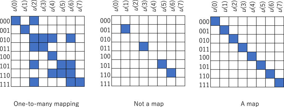
Figure 1. Examples of the input‒output table showing one-to-many type mapping, not a map, and a map in the form of an input triplet to an output triplet.

A binary sequence is expressed as a sequence of $a_i^t\in \left\{0,1\right\},i=1,2,\dots ,N$. Given a binary sequence $a_i^0\in \left\{0,1\right\},i=1,2,\dots ,N$, the input‒output table is applied to a binary sequence, and binary generation at the next step is carried out. Since a binary relation assigns an input as a triplet of binary states, a binary state is divided into a series of triplets such as $\left(a_1^t,a_2^t,a_3^t\right),\left(a_4^t,a_5^t,a_6^t\right),\dots$. The method of application is divided into two cases with respect to the style of the input‒output tables: 1) map style and 2) one-to-many type map style.

The method of application for the map style is expressed as

$a_i^{t+1}=d_0,a_{i+1}^{t+1}=d_1,a_{i+2}^{t+1}=d_2,(2)$

$i\%3=0$

where $a_i^t=c_0$, $a_{i+1}^t=c_1$, $a_{i+2}^t=c_2$, $x={\displaystyle {\sum }_{k=0}^2}{2}^{2-k}{c}_k$, $xRu\left(x\right)$, and

$u\left(x\right)=d_0{d}_1{d}_2.(3)$

For instance, if $a_{15}^t=1$, $a_{16}^t=1$, and $a_{17}^t=0$, for $15\%3=0$, then $x=6$. If $u\left(6\right)=001$, the next states are obtained as $a_{15}^{t+1}=0,a_{16}^{t+1}=0,a_{17}^{t+1}=1.$

The method of application for the one-to-many type map style is divided into two rules: a deterministic rule and a stochastic rule. Given the input‒output table as $xRu\left(x_1\right),xRu\left(x_2\right),\dots ,xRu\left(x_m\right)$, the possible next states are $u\left(x_1\right),u\left(x_2\right),\dots ,u\left(x_m\right)$, and one of the possible states is determined as the next state. First, a deterministic rule is defined. The next state is determined dependent on the neighbors of the triplet. If $2^{2\left(n-1\right)}<m\le 2^{2n}$, the $n$ number of neighbors is used to determine the next state. If $a_i^t=c_0$, $a_{i+1}^t=c_1$, $a_{i+2}^t=c_2$, $i\%3=0$, and $x={\displaystyle {\sum }_{k=0}^2}{2}^{2-k}{c}_k$, $2^{2n}$ number $2n$-bit binary sequences are divided into $m$ number sets, $D_1,D_2,\dots ,D_m$. That is the definition of the deterministic rule of the method of application for the one-to-many type map style. If

$\left(a_{i-n}^t,a_{i-n+1}^t,\dots ,a_{i-1}^t,a_{i+3}^t,a_{i+4}^t,\dots ,a_{i+3+n}^t\right)\in D_s(4)$

with $s\in \left\{1,2,\dots ,m\right\}$, $a_i^{t+1}=d_0$, $a_{i+1}^{t+1}=d_1$, and $a_{i+2}^{t+1}=d_2$, where

$u\left(x_s\right)=d_0{d}_1{d}_2.(5)$

By the stochastic rule, one of the possible states, $u\left(x_1\right),u\left(x_2\right),\dots ,u\left(x_m\right)$ is chosen, dependent on the probability function $P\left(k\right),k=1,2,\dots ,m$ with ${\displaystyle {\sum }_{k=1}^m}P\left(k\right)=1$.

Figure 2 shows an example of the deterministic rule of the method of application for the one-to-many type map. The right diagram is the input‒output table, where input triplets are arranged vertically and out triplets are arranged horizontally, at the location of which the input triplet has a relation to the output triplet, a pair of input and output triplets, and its neighbors. It is clear that $000R000,000R101,000R110$, and $000R111$. This implies that 000 can be transitioned to four possible outputs, namely, 000, 101, 110, and 111. Because $2^{2\left(n-1\right)}<4\le 2^{2n}$ is satisfied by $n=1$, binary states of ($a_{i-1}^t,$ $\left.a_{i+3}^t\right)$ are divided into four sets, $D_1=\left\{\left(0,0\right)\right\}$, $D_2=\left\{\left(0,1\right)\right\}$, $D_3=\left\{\left(1,0\right)\right\}$, and $D_4=\left\{\left(1,1\right)\right\}$. Thus, dependent on the state of the neighbors of the triplet, the next triplet is deterministically obtained. The left diagrams of Figure 2 show four different time developments of binary sequences generated by the input‒output table with a deterministic rule. The numbers surrounded by red lines represent some examples of applications of the input‒output table with deterministic rules.

Figure 2

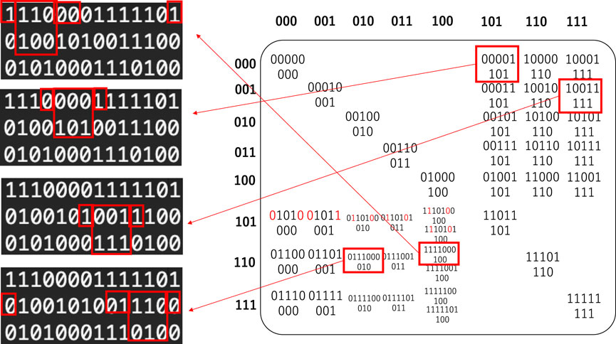
Figure 2. Illustration of the method of application for the one-to-many type map, deterministic rule. The left diagrams show some examples of time development generated by the input‒output table in which the deterministic rule is described at the location of the relation, such as $000R000$.

Similarly, it is clear that $110R000,110R001,110R010,110R011,110R100$, and $110R110$ and that 110 can transition to six possible triplets. Since $2^{2\left(n-1\right)}<6\le 2^{2n}$ is satisfied by $n=2$, binary states of (${a_{i-2}^t,a}_{i-1}^t,$ $\left.a_{i+3}^t,a_{i+4}^t\right)$, that is, 16 binary sequences, are divided into six sets:

$D_1=\left\{\left(0,0,0,0\right),\left(0,0,0,1\right),\left(1,0,0,0\right),\left(1,0,0,1\right)\right\}=\left\{\left(0,0\right)\right\},(6)$

$D_2=\left\{\left(0,0,1,0\right),\left(0,0,1,1\right),\left(1,0,1,0\right),\left(1,0,1,1\right)\right\}=\left\{\left(0,1\right)\right\},(7)$

$D_3=\left\{\left(0,1,0,0\right)\right\},(8)$

$D_4=\left\{\left(0,1,0,1\right)\right\},(9)$

$D_5=\left\{\left(1,1,0,0\right),\left(1,1,0,1\right)\right\},(10)$

$D_6=\left\{\left(0,1,1,0\right),\left(0,1,1,1\right),\left(1,1,1,0\right),\left(1,1,1,1\right)\right\}=\left\{\left(1,1\right)\right\}.(11)$

We note that $D_1=\left\{\left({a_{i-2}^t,a}_{i-1}^t,a_{i+3}^t,a_{i+4}^t\right)|\left(0,0,0,0\right),\left(0,0,0,1\right),\left(1,0,0,0\right),\left(1,0,0,1\right)\right\}=\left\{\left(a_{i-1}^t,a_{i+3}^t\right)\left.\right|\left(0,0\right)\right\}$ and all combinations of $\left(a_{i-2}^t,a_{i+4}^t\right)$ are contained and redundant and thus, omitted. $D_2$ and $D_6$ are the same situation. Each $D_k$ corresponds to $R\left(x_k\right)$; $D_1$ to $R\left(x_1\right)=000,D_2$ to $R\left(x_2\right)=001$, $D_3$ to $R\left(x_3\right)=010$, $D_4$ to $R\left(x_4\right)=011$, $D_5$ to $R\left(x_5\right)=100$, and $D_6$ to $R\left(x_6\right)=110$. The application of the deterministic rule is shown in the time development shown in the left diagram of Figure 2. See the numbers surrounded by red lines at the bottom. Since $a_i^t=1$, $a_{i+1}^t=1$, $a_{i+2}^t=0$, and (${a_{i-2}^t,a}_{i-1}^t,$ $a_{i+3}^t,a_{i+4}^t)=\left(0,1,0,0\right)\in D_3$, the next triplet is $R\left(x_3\right)=010$, and then, $a_i^t=0$, $a_{i+1}^t=1$, and $a_{i+2}^t=0$.

2.2 Logic in the form of a lattice entailed by an input‒output table

Any binary table entails logic in terms of lattice theory (Davey and Priestley, 2002). Although most researchers studying complex systems are not familiar with lattice theory, a lattice is compact and useful for estimating the logical structure. The states of dynamical systems are usually defined by integers or real numbers that constitute a totally ordered set. While any two elements, $x$ and $y$, exist in a totally ordered set, $x\le y$ or $y\le x$. Thus, one can estimate the states with respect to quantity. Partially ordered sets are generalized from totally ordered sets, where some elements, $x$ and $y$, may be neither $x\le y$ nor $y\le x$, which implies differences in quality. One can say that a partially ordered set deals not only with quantity but also quality. Strictly speaking, the order relation is defined as follows. For any elements $x,y,z$ in $P$,

$x\le x,(12)$

$x\le y,y\le x\Rightarrow x=y,(13)$

$x\le y,y\le z\Rightarrow x\le z.(14)$

A set equipped with an order relation is called a partially ordered set.

If a partially ordered set, $L$, is closed with respect to two binary operations, meet and join, $L$ is called a lattice. The meet of $x$ and $y$ in $L$, represented by $x\wedge y$, is defined by $z$ in $L$

$z\le x,z\le y\Rightarrow z\le x\wedge y.(15)$

Similarly, the union of $x$ and $y$ in $L$, represented by $x\vee y$, is defined by $z$ in $L$

$x\le z,y\le z\Rightarrow x\vee y\le z.(16)$

Given a binary relation, one can obtain a lattice in various ways. The first way is a concept lattice in which an element of an object set, $O$, has a relation to an element of an attribute set, $M$, and the binary relation is called a formal context. A pair of $A\subseteq O$ and $B\subseteq M$, $\left(A,B\right)$, is called a formal concept if each element of $A$ has a relation to all elements of $B$ and vice versa. A collection of formal concepts constitutes a lattice. This implies that the formal concept is too mathematical and is not consistent with the real-world concept proposed by cognitive linguistics. The second way is abstract chemical, in which the neighborhood of chemical species is defined, and a set of internal points and closures are defined. By using these two operations, one can constitute a fixed point, and a collection of fixed points constitutes a lattice. The third way is a rough set lattice, which is consistent with the abstract chemical approach. Therefore, a rough set lattice is a universal way to construct a lattice from a binary relation.

Given a set, $S$, an equivalence relation $K$ is defined as follows. For any $x,y,z$ in $S$,

$xKx,(17)$

$xKy\Rightarrow yKx,(18)$

$xKy,yKz\Rightarrow xKz.(19)$

The expression $xKy$ implies that $x$ is equivalent to $y$ in terms of $K$. A set consisting of equivalent elements in terms of $K$ is called an equivalent class, and such a set is defined as

${\left[a\right]}_K=\left\{x\in S|xKa\right\}.(20)$

By using an equivalent class such as neighborhood, in a term of rough set (Yao, 2004; Gunji and Haruna, 2010), upper approximation, $K^{*}\left(X\right)$, and lower approximation, $K_{*}\left(X\right)$, of $X\subseteq S$ are defined by

$K^{*}\left(X\right)=\left.\left\{x\in S\right.\right|{\left[x\right]}_K\bigcap X\ne \left.\varnothing \right\},(21)$

$K_{*}\left(X\right)=\{x\in \left.S\right|{\left[x\right]}_K\subseteq \left.X\right\}.(22)$

It is easy to see that the upper and lower approximations of $X$ correspond to necessary and sufficient conditions for $X$ since

$K_{*}\left(X\right)\subseteq X\subseteq K^{*}\left(X\right).(23)$

Therefore, the necessary and sufficient condition for $X$ in terms of $K$ is expressed as $K_{*}\left(K^{*}\left(X\right)\right)=X$. It is easy to verify that a collection of fixed points is a lattice, expressed as

$L_K=\{X\subseteq \left.S\right|K_{*}\left(K^{*}\left(X\right)\right)\left.=X\right\}.(24)$

This lattice consists of subsets of $S$, and the order relation is defined by inclusion. It is easy to see that inclusion satisfies conditions (17)–(19). For any equivalent class that satisfies $K_{*}\left(K^{*}\left(X\right)\right)=X$, any combinations of equivalent classes (i.e., union of equivalent classes) are elements of a lattice, $L_K$. A true subset of the equivalent class never satisfies $K_{*}\left(K^{*}\left(X\right)\right)=X$. $Y\subset {\left[x\right]}_K$, $K^{*}\left(Y\right)={\left[x\right]}_K$, and $K_{*}\left(K^{*}\left(X\right)\right)=$ ${\left[x\right]}_K\ne Y$. Therefore, the least elements (i.e., atoms), except for the empty set, in the lattice are equivalent classes. This implies that there exists both a union of and an intersection of any two elements of a lattice and that meet and join can be expressed as an intersection and union, respectively. In other words, lattice $L_K$ is a set lattice that is based on set theory.

Given a binary relation, one can regard a row element as an equivalent class of $K$ and a column element as an equivalent class of another equivalent class $T$. It can also be verified that

$L_{KT}=\{X\subseteq \left.S\right|K_{*}\left(T^{*}\left(X\right)\right)\left.=X\right\}(25)$

is a lattice, called a rough set lattice. While $K$ and $T$ are different equivalent relations, $L_{KT}$ is not generally a set lattice.

${\left[x\right]}_{K}I{\left[y\right]}_T:\iff \exists z\in S\left(z\in {\left[x\right]}_K,z\in {\left[y\right]}_T\right).(26)$

In the left-hand side of Figure 3, if ${\left[x\right]}_{K}I{\left[y\right]}_T$, the corresponding cell is painted blue; otherwise, it is blank. Thus, $T^{*}\left(X\right)$ is a collection of ${\left[y\right]}_T$ that has a relation to elements of $X$. If $X=\left\{a,b\right\}$, then $T^{*}\left(\left\{a,b\right\}\right)=\left\{A,B,C\right\}$ for $aIA,aIC$ and $bIB$. In contrast, $K_{*}\left(Y\right)$ is a collection of ${\left[x\right]}_K$ whose all relations are included in $Y$ (i.e., ${\left[x\right]}_K$, which has no relation to elements other than $Y$). If $Y=\left\{A,B,C\right\}$, then $K_{*}\left(\left\{A,B,C\right\}\right)=\left\{a,b\right\}$ since $aIA,aIC$ and $bIB$, and $c$ and $d$ have a relation to elements other than $\left\{A,B,C\right\}$ (e.g., $cID,dID$). Finally, one can see that $K_{*}\left(T^{*}\left(\left\{a,b\right\}\right)\right)=\left\{a,b\right\}$, which implies that $\left\{a,b\right\}$ is an element of the lattice.

Figure 3

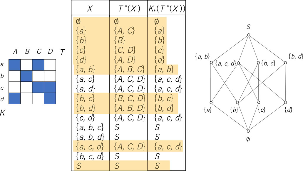
Figure 3. Construction of a lattice in the form of $L_{KT}=\left\{X\subseteq S|K_{*}\left(T^{*}\left(X\right)\right)=X\right\}$. From a binary relation between equivalence classes of $K$ and $T$ defined in a set $S$ (left), for all subsets of $S$, $K_{*}\left(T^{*}\left(X\right)\right)$ are calculated in a table, where subsets satisfying a fixed point are highlighted (center). The corresponding lattice is shown in the form of a Hasse diagram (right). See the text for details.

The right-hand side of Figure 3 shows a graphical display of the corresponding lattice in the form of a Hasse diagram. Each element of a lattice is represented by a circle accompanied by the name of the corresponding element. If one element is smaller than the other and if there is no element between the two, two elements are linked by a line, where the smaller element is located lower than the other.

As mentioned above, given a binary relation, one can obtain a lattice. In terms of a rough set lattice, rows and columns are regarded as different equivalent classes. In other words, rows and columns show two kinds of partitions based on different equivalent relations. Therefore, given an input‒output table, input triplets and output triplets are regarded as different kinds of partitions, $K$ and $T$ of a virtual world, and then, $K_{*}\left(T^{*}\left(X\right)\right)=X$ is a structure by which different partitions are connected to each other, which is nothing but a logical structure of dynamics.

3 Quantum logic automata

3.1 Traumatic relations and orthomodular lattice

Some of the input‒output tables entail quantum logic or orthomodular lattice. First, the orthocomplemented lattice is defined. A lattice $L$ is an orthocomplemented lattice if and only if for any $a\in L$ there exists $a^{\perp }\in L$ such that

$a\wedge a^{\perp }=0\text{\hspace{0.17em}or\hspace{0.17em}}a\vee a^{\perp }=1,(27)$

$a\le b\Rightarrow b^{\perp }\le a^{\perp },(28)$

$a^{\perp \perp }=a.(29)$

The distributive lattice is also defined. For any $a,b,c\in L$, a lattice,

$a\wedge \left(b\vee c\right)=\left(a\wedge b\right)\vee \left(a\wedge c\right).(30)$

$L$ is a distributive lattice. Indeed, a lattice $L$ is a complemented lattice, if and only if for any $a\in L$, there exists $a^{\perp }\in L$ such that

$a\wedge a^{\perp }=0\text{\hspace{0.17em}and\hspace{0.17em}}a\vee a^{\perp }=1.(31)$

In particular, a distributive and complemented lattice is called a Boolean lattice.

Finally, we define an orthomodular lattice. An orthocomplemented lattice $L$ is an orthomodular lattice if and only if

$a\le b\Rightarrow b=a\bigvee \left(b\bigwedge a^{\perp }\right)(32)$

for $\forall a,b\in L,a^{\perp }\in L$. An orthomodular lattice is called quantum logic. Now, all background details are prepared (Gunji and Nakamura, 2022).

Here, we define quantum logic automata. Quantum logic automata are the logic automata whose input‒output table entails quantum logic. Figure 4 illustrates two examples of quantum logic automata. It is easy to construct an input‒output table whose corresponding lattice is an orthomodular lattice. Given an $8\times 8$ binary relation, $I$, in which each row is represented by $a_k,k=1,2,\dots ,8$, which is an equivalence class of equivalence relations, $K$, on a set $S$, and each column is represented by $A_k,k=1,2,\dots ,8$, which is an equivalence class of equivalence relations, $T$, on a set $S$, if the relation consists of diagonal relations with $m\times m$, $2\le m\le 6$, and the background of the diagonal relations is filled with $a_{p}I{A}_q$, the relation is called the traumatic relation and entails an orthomodular lattice. Here, the $m\times m$ diagonal relation is defined by $k=1+s,2+s,\dots ,m+s$, $a_{k}I{A}_k$, and if $p\ne q$, $a_p$ has no relation to $A_q$. In that sense, the two input‒output tables shown in Figure 4 are traumatic relations (also see Gunji et al., 2022; Gunji and Haruna, 2022; Gunji and Nakamura, 2022; 2023).

Figure 4

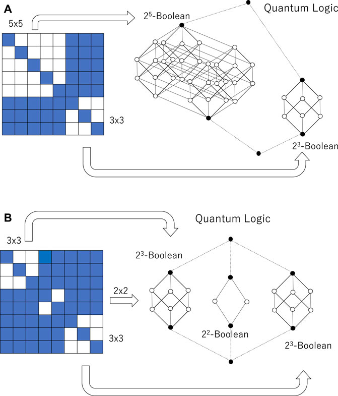
Figure 4. Two quantum logic automata entailing orthomodular lattices. (A) An orthomodular lattice is constructed as an almost disjoint union of 2⁵- and 2³-Boolean algebras. (B) An orthomodular lattice is constructed as an almost disjoint union of two 2³- and 2²-Boolean algebras.

It is easy to see that the traumatic structure entails the orthomodular lattice. Let us consider the binary relation shown in Figure 4A. We confirm that the $5\times 5$ diagonal relation is surrounded by relations to $\left\{A_6,A_7,A_8\right\}$. Thus, for a subset of $\left\{a_1,a_2,{\dots ,a}_5\right\}$ such as $\left\{a_1,a_2\right\}$,

$\left.T^{*}\left(\left\{a_1,a_2\right\}\right)={\left\{A_1,A_2\right\}\cup \left\{A\right.}_6,A_7,A_8\right\},(33)$

and then

$K_{*}\left(\left.{\left\{A_1,A_2\right\}\cup \left\{A\right.}_6,A_7,A_8\right\}\right)=\left\{a_1,a_2\right\}.(34)$

This implies that $\left\{a_1,a_2\right\}$ is a fixed point satisfying $K_{*}\left(T^{*}\left(X\right)\right)=X$. While this can be generalized to any true subset of $\left\{a_1,a_2,{\dots ,a}_5\right\}$, the set, $\left\{a_1,a_2,{\dots ,a}_5\right\}$, never satisfies $K_{*}\left(T^{*}\left(X\right)\right)=X$ because $K_{*}\left(T^{*}\left(\left\{a_1,a_2,{\dots ,a}_5\right\}\right)\right)=K_{*}\left(S\right)=S$. Any subsets of $S$ consisting of components of different diagonal relations such as $\left\{a_1\right\}\cup \left\{a_8\right\}$ also do not satisfy $K_{*}\left(T^{*}\left(X\right)\right)=X$.

From these considerations, one can say that any diagonal relation entails a set lattice, which is a Boolean algebra where the least element is an empty set and the greatest element is $S$. In other words, each Boolean sublattice shares the greatest and least element. In Figure 4, the solid line represents the order relation, while the broken line connecting black circles represents the equivalent relation. Therefore, Figure 4 shows that the traumatic relation entails a lattice consisting of multiple Boolean algebras sharing the greatest element represented by 1 and least element represented by 0.

The lattice is an orthomodular lattice. For a Boolean lattice that is a complementary lattice, one can define an orthocomplement by the complement satisfying conditions (27) and (29) in each Boolean sublattice. Except for the least and the greatest elements, if one of the two elements is larger than the other, those two belong to the same Boolean sublattice. Therefore, $a\le b$ implies $a\wedge b=a$ and $a^{\perp }={\left(a\wedge b\right)}^{\perp }=a^{\perp }\vee b^{\perp }$ because condition (30) holds in Boolean algebra, and then, $a^{\perp }\wedge b^{\perp }=\left(a^{\perp }\vee b^{\perp }\right)\wedge b^{\perp }=b^{\perp }$. This finding verifies $a\le b\Rightarrow b^{\perp }\le a^{\perp }$, condition (28). This implies that the lattice is an orthocomplemented lattice. Condition (32) can be verified similarly. Since $a\le b$ and they belong to the same Boolean sublattice, $a\bigvee \left(b\bigwedge a^{\perp }\right)=\left(a\bigvee b\right)\wedge \left(a\vee a^{\perp }\right)=b\wedge 1=b$. This implies that $a\le b\Rightarrow b=a\bigvee \left(b\bigwedge a^{\perp }\right)$, condition (32). Thus, an orthocomplemented lattice is an orthomodular lattice. Finally, one can say that the traumatic relation entails an orthomodular lattice, i.e., quantum logic.

Here, we call the logic automata whose input‒output table is the traumatic relation quantum logic automata. In quantum logic, the distributive law in the form of (30) does not hold for elements belonging to different Boolean sublattices. In contrast, the distributive law holds in Boolean algebra. If the input‒output table consists of one diagonal relation, it entails a Boolean lattice. For this case, we call it Boolean logic automata.

3.2 The behavior of quantum logic automata

Here, we show the behavior of quantum logic automata compared with that of the Boolean logic automata. Figure 5 shows a schematic diagram of the input‒output table and the method of application. Since the input‒output table is applied to a binary sequence, for every triplet without overlapping, the background of the diagonal relation plays an essential role in the interactions of triplets. In Figure 5, triplet 001, for instance, can transit to four possible triplets, $\left(1\right),u\left(5\right),u\left(6\right),u\left(7\right)$, depending on the state of the neighbors of the triplet. Therefore, due to the dependency on the state of the neighbors, the triplet can interact with each other.

Figure 5

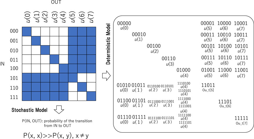
Figure 5. Input‒output table and the method of application for quantum logic automata. The output values, $u\left(k\right),k=0,1,...,7$, are defined by a triplet of 0 and 1. The right table of the method of application corresponds to the input‒output table. See the text for details.

Compared to quantum logic automata, Boolean logic automata cannot realize the interactions among triplets. While quantum logic automata reveal a one-to-many type map style with respect to triplets, Boolean logic automata reveal a map since the transit of a triplet is uniquely determined. That is why the time development of the binary sequence generated by Boolean logic automata converges into locally stable oscillations, with at most eight states per period. In terms of classifications of cellular automata, patterns generated by Boolean logic automata belong to class II. What is the pattern generated by quantum logic automata? Even if the same triplets are given for $\left(k\right),k=0,1,...,7$, the patterns generated by quantum logic automata are different from those generated by Boolean logic automata.

Figure 6 shows the patterns generated by quantum logic automata compared to those generated by Boolean logic automata, where the value of $u\left(k\right),k=0,1,...,7$ is common to both logic automata. The patterns shown in Figure 6A are typical patterns generated by quantum logic automata and are similar to patterns generated by cellular automata assigned by class IV. Periodic waves from the right to the left propagate, and the collisions of waves lead to complex behaviors. In particular, the patterns generated by quantum logic automata in Figure 6A reveal a complex background pattern that consists of dense oscillatory waves propagating from left to right. Thus, the inference between the propagating waves and background waves also leads to complex behavior.

Figure 6

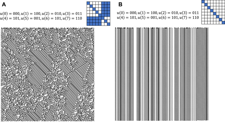
Figure 6. Patterns generated by quantum logic automata (A) and Boolean logic automata (B) under the same $u\left(k\right),k=0,1,...,7$. Boundary conditions are periodic boundaries. The binary relations shown above correspond to the input‒output table for quantum logic automata and Boolean logic automata. In the generated patterns, a state of 1 is represented by a black square and 0 by a blank, where the horizontal line represents space and the vertical line represents time.

As mentioned before, patterns generated by Boolean logic automata display patterns generated by cellular automata assigned by class II. Since $u\left(k\right),k=0,1,...,7$ are common to both logic automata, the complex behavior found in quantum logic automata may result from multiple transitions appearing in the input‒output table of quantum logic automata. Locally stable oscillations found in patterns generated by Boolean logic automata (Figure 6B) are propagated diagonally depending on the neighbors of the oscillatory state and generate propagating waves, collision of waves, and very complex behavior.

Class IV-like behavior is not a rare case in quantum logic automata. To estimate it with respect to the pattern in appearance, a collection of quantum logic automata is systematically constructed. The input‒output table and the method of application are shown in Figure 5, where $u\left(k\right),k=0,1,...,7$ is randomly determined as one of $\left\{000,001,\dots ,111\right\}$ to make $u:\left\{0,1,\dots ,7\right\}\to \left\{000,001,\dots ,111\right\}$ bijective. Once $u\left(k\right),k=0,1,...,7$ is randomly determined, time development for the rule is generated. Two hundred samples of rules are collected, and the time development patterns are classified, as shown in Figure 7. It results in 17% of the samples as class II, 5% as class III, and most of the samples, 78%, as class IV.

Figure 7

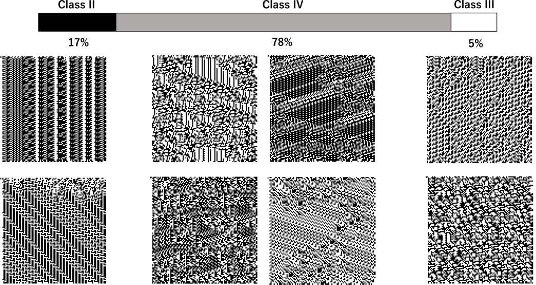
Figure 7. Percentage of class II, III, and IV patterns generated by quantum logic automata (above) and time development generated by quantum logic automata showing class II (left two patterns), class IV (central four patterns), and class III (right two patterns).

Classification with respect to the pattern in appearance seems not to be arbitrary. The percentage of class IV might be much higher. The class II pattern is characterized by locally stable oscillations that propagate either vertically or diagonally. Because the pattern is identified with class II, whether the transient time is long or short, potential class IV might be included in class II. The class IV pattern is characterized by interactions of multiple propagating waves that oscillate. Some waves are propagated vertically, and some are propagated diagonally. The collision of waves leads to a complex shift in the propagating direction and/or a period of oscillation. Patterns in which it is not easy to find multiple propagating waves are identified as class III. Therefore, potential class IV might be included in class III. The time development of class III shown in Figure 7 reveals such a property. Although it is difficult to determine, a pattern consists of waves propagating vertically.

Figure 8 shows examples of a pair of time developments generated by quantum logic automata and Boolean logic automata, where the pattern of quantum logic automata shows class IV. The input‒output table and the method of application are shown in Figure 5, and $u\left(k\right),k=0,1,...,7$ is randomly determined as a bijective map from $\left\{0,1,\dots ,7\right\}$ to $\left\{000,001,\dots ,111\right\}$. It is easy to see that there are vertically propagating waves and diagonally propagating waves that sometimes collide with each other. Collisions lead to various interferences, such as changes in the propagating direction, velocity, and/or period of oscillation. A pattern left and the third from the top and a pattern right and top in Figure 8 show the velocity change in diagonally propagating waves after the collision. The right and second patterns from the top show the shift in the propagating direction of the vertical wave after the collision. Other various patterns show the change in the period of oscillation and the amplitude of the waves after the collision.

Figure 8

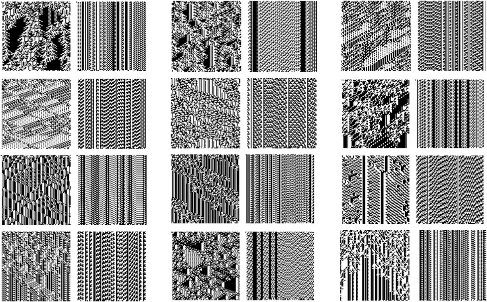
Figure 8. Comparison of patterns generated by quantum logic automata and Boolean logic automata. In each pair, the left diagram shows the pattern generated by quantum logic automata, and the right diagram shows the pattern generated by Boolean logic automata.

When a pattern generated by quantum logic automata is compared to a pattern generated by Boolean logic whose $u\left(k\right)$ is the same as that of quantum logic automata, one can see that the locally stable oscillation found in a pattern of Boolean logic automata is propagated diagonally in a pattern of quantum logic automata. If broad black massive patterns are stable in a pattern of Boolean logic automata, massive black patterns are found as the background in which traveling waves are propagated in a pattern of quantum logic automata. They are illustrated in patterns in the top left and central, in the second from the top right, and in bottom central in Figure 8. Periodic oscillations found in a pattern of Boolean logic automata are found in oscillatory traveling waves in quantum logic automata, for instance, in patterns located left the second and fourth from the top and located center the second from the top in Figure 8. Periodic oscillations found in a pattern of Boolean logic automata are sometimes found as the background pattern in a pattern of quantum logic automata and are illustrated in the patterns located right the third from the top in Figure 8. From these observations, it is clear that patterns generated by quantum logic automata are influenced by patterns generated by Boolean logic automata.

The next question arises regarding the property of critical phenomena or the edge of chaos. To estimate this property, the power spectrum of a time series of time development is estimated here. Because the power-law in a time series is found in class IV with respect to the time series of the number of state 1 at each time step, the value, $c\left(t\right)$, at each time step of the binary sequence is defined as

$c\left(t\right)=\frac{1}{N}{\displaystyle {\sum }_{i=1}^N}{a}_i^t.(35)$

For some class IV patterns found in quantum logic automata that consist of traveling waves and an oscillatory background, binary sequences are modified by the filter, such as

$\left(a_i^t=1,a_{i+1}^t=1,a_{i+2}^t=0\right)\to \left(b_i^t=0,b_{i+1}^t=0,b_{i+2}^t=0\right),(36)$

$\left(a_i^t=0,a_{i+1}^t=1,a_{i+2}^t=1\right)\to \left(b_i^t=0,b_{i+1}^t=0,b_{i+2}^t=0\right).(37)$

The modification of values (i.e., filtering [Boccara et al., 1991; Martinez et al., 2006]) in (36) and (37) never reflects the time development, and the value at each time step is expressed as

$c^{fileterd}\left(t\right)=\frac{1}{N}{\displaystyle {\sum }_{i=1}^N}{b}_i^t.(38)$

Due to the filtering, a time series of binary sequences is evaluated to focus on the interactions of oscillatory traveling waves, which is nothing but a characteristic of the class IV pattern. The equations of filtering are not universal and must be defined depending on the background pattern generated by quantum logic automata.

Figure 9 shows some results of power spectrum analysis for a filtered time series of binary sequences generated by quantum logic automata. The input‒output table and the method of application are given in Figure 5, and $u:\left\{0,1,\dots ,7\right\}\to \left\{000,001,\dots ,111\right\}$, which is bijective, is randomly determined. In particular, the rule by which a pattern shown in Figure 9 on the left is expressed as $u\left(0\right)=010,u\left(1\right)=100,u\left(2\right)=000,u\left(3\right)=110,u\left(4\right)=001,u\left(5\right)=011,u\left(6\right)=101,u\left(0\right)=111$. The amplitude of the spectrum, $A$, shows a power-law distribution dependent on frequency, $\nu$, such that

$A\propto {\nu }^{-\alpha }.(39)$

Figure 9

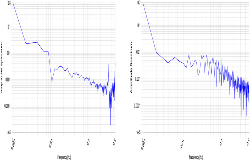
Figure 9. Power spectrum of a time series of Eq. 38 generated by quantum logic automata.

In the case of the power spectrum shown on the left-hand side of Figure 9, $\alpha =1.01$ for the low-frequency components. Any other power spectrum for the time series generated by quantum logic automata generally shows a power-law distribution if patterns show class IV behavior. From these observations, one can say that quantum logic automata generate class IV-like behaviors that are characterized by complex interactions of oscillatory traveling waves and display a power-law distribution, which is the essential property of the edge of chaos or critical phenomena.

4 Discussion

Scale-free properties suggesting critical phenomena and/or the edge of chaos are generally found in natural biological phenomena, including brain activity (Fontenele et al., 2018; Lender et al., 2020, Jannessai et al., 2020, Toker, et al., 2022). Although various attempts have been made to generalize the idea of the edge of chaos, most attempts conversely claim that the edge of chaos is so rare that natural selection essentially plays a role in choosing the natural biological phenomena at the edge of chaos (Bak et al., 1987; Bak and Tang, 1989; Bak and Sneppen, 1993; Sneppen et al., 1995; Kauffman and Johnsen, 1991;). Since the idea of a wedged landscape and self-organized criticality is implemented in the form of nonlinear dynamics, chaotic behavior must be balanced with oscillatory order through the rugged boundary by which attractors are isolated.

The classification of cellular automata also claims that class IV cellular automata located at the boundary between classes I and II (order) and class III (chaos) are very rare and that class IV automata can be at the critical state of the phase transition (Langton, 1990; Wolfram, 2002; Barbu, 2013). It has also been verified that a universal Turing machine can be implemented by class IV elementary cellular automata (Cook, 2004), which suggests that class IV cellular automata have high computability. While class IV cellular automata might be relevant for self-organized criticality, a power-law distribution was discovered very recently.

While the idea of the edge of chaos or self-organized criticality is specific but displays the power-law distribution, the ideas of homeochaos and/or Markov blanket do not show power-law distribution, notwithstanding claiming that it is proposed as a general theory. On the other hand, the newly defined Markov blanket (Friston et al., 2021) might not be generalized as the interface connecting the external environment and empirical world due to the specific recurrent structure. In that sense, while it shows scale-free connectivity, it is too specific to claim general theory.

Figure 10 shows a schematic diagram of various theories relevant for the interface between chaos and order. Various theories are plotted in the phase space, where the horizontal line represents generality and the vertical line represents rigor. While the idea of the edge of chaos and self-organized criticality is rigorously constructed in the form of nonlinear dynamics to show the power-law distribution, they lose generality. That is why they are located at high rigor plotted against low generality. In contrast, homeochaos and Markov blanket are located at low rigor plotted against high generality in the phase space, as shown in Figure 10. In that sense, one might see the trade-off between the rigor and generality of the theories relevant for the behavior in which order and chaos coexist. That trade-off might be found in the “normal” idea of complex systems. The term “normal” suggests synchronous updating in discrete dynamics and nonlinear dynamics isolated from perturbation.

Figure 10

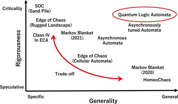
Figure 10. Schematic diagram of the trade-off between rigorousness and generality in the model revealing the edge of chaos and/or criticality. Quantum logic automata might break the trade-off.

One of the potential candidates breaking the trade-off is asynchronous cellular automata. In asynchronously updated automata, various ways of updating are proposed such that only some randomly determined cells are updated at each step (Fatès et al., 2006; Fatès, 2014), the order of updating is randomly determined at each time step (Gunji, 1990; Gunji and Uragami, 2020), and the two kinds of updating interact with each other (Gunji, 2015; Uragami and Gunji, 2018; Gunji and Uragami, 2021; Uragami and Gunji, 2022). The third implementation is called asynchronously tuned automata. Due to asynchronous updating, multiple rules are mixed up as the transition rule, even if the transition rule is uniquely determined. This results in various rules appearing randomly in time and space. In that sense, dynamics itself contains the interface of chaos and order. Indeed, even if some transition rules show various behaviors such as classes I, II, and III, the devices of asynchronous updating entail class IV behavior, accompanied by the power-law distribution. This suggests that asynchronous cellular automata might break the trade-off to some extent.

From these considerations, one can say that quantum logic automata break the trade-off between rigor and generality. Figure 7 shows the percentage of order, chaos, and critical behavior of quantum logic automata. If quantum logic automata show similar tendencies of elementary cellular automata, class IV behaviors are destined to be rare. However, most of the rules in the quantum logic automata defined by Figure 5 show class IV behavior, which is characterized by the collision and interactions among oscillatory traveling waves. Indeed, quantum logic automata showing class IV behavior show a power-law distribution in the form of $1/f$ noise. These observations show that quantum logic automata are located at high rigor against high generality in the phase space of rigor and generality (Figure 10).

Although quantum logic automata are variously defined, the whole behavior of quantum logic automata is still unclear. Only one input‒output table revealing traumatic relations is discussed in this paper. There are various traumatic relations that are to be estimated as quantum logic automata. Even if the input‒output table is uniquely given, there are many methods of applications since there are various ways assigning the states of neighbors into the output. We used only one method of application in this paper.

How is the traumatic relation generated entailing quantum logic? We previously showed that inverse and/or excess Bayesian inference can lead to a traumatic structure. The traumatic structure consists of multiple diagonal relations and the related background surrounding the diagonal relations. Each diagonal relation corresponds to a Boolean lattice reflecting the empirical individual world resulting from Bayesian inference, and the related background corresponds to the interface connecting multiple Boolean lattices. In that sense, a traumatic relation itself can correspond to the Markov blanket. Inverse and/or excess Bayesian inference might result in quantum logic automata as dynamics.

Our research could be related to bipolar dynamic logic (BDL) and bipolar quantum cellular automata (BQCA). BDL consists of bipolar elements, (−1, 1), (−1, 0), (0, 1), and (0, 0). In ignoring the symbol “−,”the corresponding Hasse diagram shows 2²-Boolean lattice. While binary operations defined in a lattice are only join and meet, various operations are defined in BDL. The operations & and $\oplus$ normally correspond to the meet and the join, respectively, as if the symbol “−” was ignored. The operations $\otimes$ and $\varnothing$ are newly defined to show a variety of operations (Zhang, 2013; Zhang, 2021).

Quantum mechanics has specificity compared to classical mechanics with respect to both the operand and operator. Normal lattice theory focuses on the operand, and the operator is constrained only to the join and meet. Diversity of the operand is expressed as specific elements revealing “entanglement.” Boolean lattice whose number of atoms is $n$ consists of any possible unions of atoms, and then, the number of elements is 2ⁿ. The orthomodular lattice (i.e., quantum logic) consists of some Boolean sublattices overlapping each other. In other words, there exist elements belonging to multiple Boolean sublattices that reveal the entanglement. That is why orthomodular lattice reveals the specificity of quantum mechanics with respect to the operand.

In contrast, BDL focuses on operators. The strategy focusing on the operator is also found in modal logic. Notwithstanding the 2²-Boolean lattice, closure operation is added and defined to extend the Boolean algebra. Similarly, notwithstanding 2²-Boolean lattice, &, $\oplus$, ${\&}^{-}$, ${\oplus }^{-}$, $\otimes ,\varnothing$, ${\otimes }^{-}$, and ${\varnothing }^{-}$ are defined, and that leads to show the richness of quantum mechanics with respect to the operator. Bipolar quantum linear algebra is naturally extended by replacing $\left\{-1,0\right\}\times \left\{0,1\right\}$ with $\left[-\infty ,0\right]\times \left[0,+\infty \right]$. These extensions can make it possible to define tensor multiplication and addition. In that sense, a variety of operators are added.

By using a rough set lattice, our approach shows how an orthomodular lattice results from combining Boolean lattices. Boolean lattice corresponds to classical logic and/or classical mechanics, and it is clear to see how orthomodular lattice and Boolean lattice are unified. Indeed, our approach is related to the dynamical system in terms of cellar automata and shows that the orthomodular lattice entails irreversible complex behavior or a non-equilibrium system, and the Boolean lattice entails reversible simple behavior or an equilibrium system.

Our approach claims that multiple Boolean lattices are connected via the “entanglement,” and the time development of quantum cellular automata transients from one Boolean lattice to another and vice versa. A single Boolean lattice (i.e., classical mechanics) implies a dynamical system, revealing one-to-one mapping, and that implies order (classes I and II) in terms of cellular automata. Therefore, quantum cellular automata could transient from one Boolean lattice to multiple Boolean lattices via entanglement, which implies one-to-many type mapping. Thus, quantum cellular automata can reveal the intermediate dynamics consisting of order and disorder or class IV behavior in terms of cellular automata. Our approach is consistent with bipolar quantum geometry and can focus on the operand compared to the bipolar quantum approach focusing on the operator.

5 Conclusion

While a diagonal relation entails Boolean logic, a traumatic relation consisting of multiple diagonal relations and related background entails quantum logic. On one hand, the conflict between Boolean logic and quantum logic reveals the conflict between quantum cognition and the free energy principle in cognitive and brain science. On the other hand, it reveals the conflict of open-ended dynamics and steady-state dynamics. Although open-ended dynamics can be strongly relevant for the idea of the edge of chaos, self-organized criticality, and a power-law distribution, no theory of quantum cognition has been proposed to reveal a power-law distribution.

To clarify the relationship between quantum logic and the edge of chaos, we propose quantum logic automata. The binary relation used as the input‒output table entails quantum logic; if the binary relation is applied to a binary sequence, then the time development of the binary sequence is generated. The method of application is defined by a deterministic rule and a stochastic rule. In particular, we discuss the behaviors of quantum logic automata implemented by deterministic rules in which one of the possible multiple outputs is deterministically determined depending on the state of neighbors.

Here, we show that most quantum logic automata reveal class IV-like behavior characterized by the interactions of oscillatory traveling waves and reveal a power-law distribution in the form of $1/f$ noise. This suggests that quantum logic as a dynamical system features chaotic transitions among multiple attractors and that the idea of self-organized criticality and/or the edge of chaos can be generalized through quantum logic or quantum theory.

Data availability statement

The original contributions presented in the study are included in the article/Supplementary Material; further inquiries can be directed to the corresponding author.

Author contributions

Y-PG: conceptualization, formal analysis, investigation, visualization, and writing–original draft. YO: conceptualization, visualization, writing–original draft, and investigation. YT: writing–original draft, conceptualization, and investigation. KE: conceptualization, investigation, and writing–original draft.

Funding

The author(s) declare that financial support was received for the research, authorship, and/or publication of this article. This work was supported by JSPS 22K12231.

Acknowledgments

The authors thank students for discussing the topic in the laboratory.

Conflict of interest

The authors declare that the research was conducted in the absence of any commercial or financial relationships that could be construed as a potential conflict of interest.

Publisher’s note

All claims expressed in this article are solely those of the authors and do not necessarily represent those of their affiliated organizations, or those of the publisher, the editors, and the reviewers. Any product that may be evaluated in this article, or claim that may be made by its manufacturer, is not guaranteed or endorsed by the publisher.

References

Abraham, F. D., Abraham, R. H., and Shaw, C. D. (1990). A visual introduction to dynamical systems theory for psychology. China: Aerial Press.

Google Scholar

Aerts, D. (2009). Quantum structure in cognition. J. Math. Psychol. 53, 314–348. doi:10.1016/j.jmp.2009.04.005

CrossRef Full Text | Google Scholar

Aerts, D., Aerts Arguëlles, J., Beltran, L., Geriente, S., Sassoli de Bianchi, M., Sozzo, S., et al. (2019). Quantum entanglement in physical and cognitive systems: a conceptual analysis and a general representation. Eur. Phys. J. Plus 134, 493. doi:10.1140/epjp/i2019-12987-0

CrossRef Full Text | Google Scholar

Aerts, D., Broekaert, J., Gabora, L., and Veroz, T. (2012). The guppy effect as interference. Quantum Interaction 2012. Germany: Springer, 36–74.

CrossRef Full Text | Google Scholar

Aerts, D., Gabora, L., and Sozzo, S. (2013). Concepts and their dynamics: a quantum-theoretic modeling of human thought. Top. Cognitive Sci. 5, 737–772. doi:10.1111/tops.12042

PubMed Abstract | CrossRef Full Text | Google Scholar

Asano, M., Khrennikov, A., Ohya, M., Tanaka, Y., and Yamato, I. (2015). Quantum adaptivity in biology: from genetics to cognition. Heidelberg-Berlin-New York: Springer.

Google Scholar

Atmanspacher, H., Römer, H., and Walach, H. (2002). Weak quantum theory: complementarity and entanglement in physics and beyond. Found. Phys. 32 (3), 379–406. doi:10.1023/a:1014809312397

CrossRef Full Text | Google Scholar

Bak, P. (1996). How nature works: the science of self-organized criticality. New York: Copernicus.

Google Scholar

Bak, P., and Sneppen, K. (1993). Punctuated equilibrium and criticality in a simple model of evolution. Phys. Rev. Lett. 71, 4083–4086. doi:10.1103/physrevlett.71.4083

PubMed Abstract | CrossRef Full Text | Google Scholar

Bak, P., and Tang, C. (1989). Earthquakes as a self-organized critical phenomenon. J. Geophys. Res. Solid Earth 94 (15), 15635–15637. doi:10.1029/jb094ib11p15635

CrossRef Full Text | Google Scholar

Bak, P., Tang, C., and Wiesenfeld, K. (1987). Self-organized criticality: an explanation of 1/f noise. Phys. Rev. Lett. 59, 381–384. doi:10.1103/physrevlett.59.381

PubMed Abstract | CrossRef Full Text | Google Scholar

Barbu, V. (2013). Self-organized criticality of cellular automata model; absorbtion in finite-time of supercritical region into the critical one. Math. Methods Appl. Sci. 36, 1726–1733. doi:10.1002/mma.2718

CrossRef Full Text | Google Scholar

Blutner, R., and beim Graben, P. (2016). Quantum cognition and bounded rationality. Synthese 193, 3239–3291. doi:10.1007/s11229-015-0928-5

CrossRef Full Text | Google Scholar

Boccara, N., Nasser, J., and Roger, M. (1991). Particle like structures and their interactions in spatio-temporal patterns generated by one dimensional deterministic cellular automaton rules. Phys. Rev. A 44 (2), 866–875. doi:10.1103/physreva.44.866

PubMed Abstract | CrossRef Full Text | Google Scholar

Boedecker, J., Obst, O., Lizier, J. T., Mayer, N. M., and Asada, M. (2012). Information processing in echostate networks at the edge of chaos. Theory Biosci. 131, 205–213. doi:10.1007/s12064-011-0146-8

PubMed Abstract | CrossRef Full Text | Google Scholar

Bruza, P. D., Wang, Z., and Busemeyer, J. R. (2015). Quantum Cognition: a new theoretical approach to psychology. Trends Cognitive Sci. 19, 383–393. doi:10.1016/j.tics.2015.05.001

PubMed Abstract | CrossRef Full Text | Google Scholar

Bunimovich, L. A., and Sinai, Y. G. (1988). Spacetime chaos in coupled map lattices. Nonlinearity 1, 491–516. doi:10.1088/0951-7715/1/4/001

CrossRef Full Text | Google Scholar

Busemeyer, J. R., and Bruza, P. D. (2012). Quantum models of cognition and decision. Cambridge: Cambridge University Press.

Google Scholar

Busemeyer, J. R., Pothos, E. M., Franco, R., Trueblood, J. S., and Trueblood, J. S. (2011). A quantum theoretical explanation for probability judgment errors. Psychol. Rev. 118 (2), 193–218. doi:10.1037/a0022542

PubMed Abstract | CrossRef Full Text | Google Scholar

Clark, A. (2017). “How to knit Your own Markov blanket,” in Philosophy and predictive processing. Editors T. K. Metzinger, and &W. Wiese (Frankfurt am Main, Germany: MIND Group).

Google Scholar

Cook, M. (2004). Universality in elementary cellular automata. Complex Syst. 15 (1), 1–40.

Google Scholar

Cordero, C. G. (2017). Parameter adaptation and criticality in particle swarm optimization. arXiv:1705.06966x1[cs.NE] May 19, 2017).

Google Scholar

Dahmen, D., Grün, S., Diesmann, M., and Helias, M. (2019). Second type of criticality in the brain uncovers rich multiple-neuron dynamics. Proc. Natl. Acad. Sci. U. S. A. 116, 13051–13060. doi:10.1073/pnas.1818972116

PubMed Abstract | CrossRef Full Text | Google Scholar

Davey, B. A., and Priestley, H. A. (2002). Intr5oduction to lattice and order. Cambridge: Cambridge Univ. Press.

Google Scholar

Erskine, A., and Hermann, J. M. (2015). CriPS: critical particle swarm optimization. Proc. Eur. Conf. Art. Life, 207–214.

Google Scholar

Fatès, N. (2014). A guided tour of asynchronous cellular automata. J. Cell. Autom. 9, 387–416.

Google Scholar

Fatès, N., Thierry, É., Morvan, M., and Schabanel, N. (2006). Fully asynchronous behavior of double-quiescent elementary cellular automata. Theor. Comput. Sci. 362, 1–16. doi:10.1016/j.tcs.2006.05.036

CrossRef Full Text | Google Scholar

Fontenele, A. J., de Vasconcelos, N. A. P., Feliciano, T., Aguiar, L. A. A., Soares-Cunha, C., Coimbra, B., et al. (2018). Criticality between cortical states. bioRxiv Prepr. doi:10.1101/454934

CrossRef Full Text | Google Scholar

Friston, K. (2019). A free energy principle for a particular physics, arXiv:1906.10184.

Google Scholar

Friston, K., Da Costa, L., and Parr, T. (2020). Some interesting observations on the free energy principle. arXiv:2002.04501.

Google Scholar

Friston, K. J. (2010). The free-energy principle: a unified brain theory? Nat. Rev. Neurosci. 11, 127–138. doi:10.1038/nrn2787

PubMed Abstract | CrossRef Full Text | Google Scholar

Friston, K. J., Fagerholm, E. D., Zarghami, T. S., Parr, T., Hipólito, I., Magrou, L., et al. (2021). Parcels and particles: Markov blankets in the brain. Netw. Neurosci. 5 (1), 211–251. doi:10.1162/netn_a_00175

CrossRef Full Text | Google Scholar

Friston, K. J., and Kiebel, S. (2009a). Cortical circuits for perceptual inference. Neural Netw. 22, 1093–1104. doi:10.1016/j.neunet.2009.07.023

PubMed Abstract | CrossRef Full Text | Google Scholar

Friston, K. J., and Kiebel, S. (2009b). Predictive coding under the free-energy principle. Philosophical Trans. R. Soc. B Biol. Sci. 364, 1211–1221. doi:10.1098/rstb.2008.0300

PubMed Abstract | CrossRef Full Text | Google Scholar

Friston, K. J., Kilner, J., and Harrison, L. (2006). A free energy principle for the brain. J. Physiology-Paris 100, 70–87. doi:10.1016/j.jphysparis.2006.10.001

PubMed Abstract | CrossRef Full Text | Google Scholar

Gunji, Y. (1990). Pigment color patterns of molluscs as an autonomous process generated by asynchronous automata. Biosystems 23, 317–334. doi:10.1016/0303-2647(90)90014-r

PubMed Abstract | CrossRef Full Text | Google Scholar

Gunji, Y. P. (2015). “Extended self-organized criticality in asynchronously tuned cellular automata,” in Chaos, information processing. Editors P. Games, G. Nicolis, and V. Basios (China: World Scientific), 411–429.

CrossRef Full Text | Google Scholar

Gunji, Y. P., and Haruna, T. (2010). A non-boolean lattice derived by double indiscernibility. Lect. Notes Comput. Sci. XII, 211–225. doi:10.1007/978-3-642-14467-7_11

CrossRef Full Text | Google Scholar

Gunji, Y. P., and Haruna, T. (2022). Concept Formation and quantum-like probability from nonlocality in cognition. Cogn. Comput. 14, 1328–1349. doi:10.1007/s12559-022-09995-1

CrossRef Full Text | Google Scholar

Gunji, Y. P., and Nakamura, K. (2022). Psychological origin of quantum logic: an orthomodular lattice derived from natural-born intelligence without Hilbert space. BioSystems 215-216, 104649. doi:10.1016/j.biosystems.2022.104649

CrossRef Full Text | Google Scholar

Gunji, Y. P., and Nakamura, K. (2023). “Kakiwari: the device summoning creativity in art and cognition,” in Unconventional computing, philosophies and art. Editor A. Adamatzky (Singapore: World Scientific), 135–168.

Google Scholar

Gunji, Y. P., Shinohara, S., and Basios, V. (2022). Connecting the free energy principle with quantum cognition. Front. NeuroRobotics 16, 910161. doi:10.3389/fnbot.2022.910161

CrossRef Full Text | Google Scholar

Gunji, Y. P., Shinohara, S., and HarunaT, B. V. (2017). Inverse Bayesian inference as a key of consciousness featuring a macroscopic quantum logic structure. BioSystems 152, 44–63.

PubMed Abstract | CrossRef Full Text | Google Scholar

Gunji, Y. P., Sonoda, K., and Basios, V. (2016). Quantum cognition based on an ambiguous representation derived from a rough set approximation. Biosystems 141, 55–66. doi:10.1016/j.biosystems.2015.12.003

PubMed Abstract | CrossRef Full Text | Google Scholar

Gunji, Y. P., and Uragami, D. (2020). Breaking of the trade-off principle between computational universality and efficiency by asynchronous updating. Entropy 22 (9), 1049. doi:10.3390/e22091049

PubMed Abstract | CrossRef Full Text | Google Scholar

Gunji, Y. P., and Uragami, D. (2021). Computational power of asynchronously tuned automata enhancing the unfolded edge of chaos. Entropy 23 (11), 1376. doi:10.3390/e23111376

CrossRef Full Text | Google Scholar

Haken, H. (1977). Synergetics. Phys. Bull. 28 (9), 412–414. doi:10.1088/0031-9112/28/9/027

CrossRef Full Text | Google Scholar

Hameroff, S. (2012). How quantum brain biology can rescue conscious free will. Front. Integr. Neurosci. 6, 93. doi:10.3389/fnint.2012.00093

PubMed Abstract | CrossRef Full Text | Google Scholar

Haven, E., and Khrennikov, A. (2013). Quantum social science. Cambridge: Cambridge University Press.

Google Scholar

Ishwarya, M. S., and Kumar, C. A. (2020a). Quantum aspects of high dimensional conceptual space: a model for achieving consciousness. Cogn. Comput. 12, 563–576. doi:10.1007/s12559-020-09712-w

CrossRef Full Text | Google Scholar

Jannesari, M., Saeedi, A., Zare, M., Ortiz-Mantilla, S., Plenz, D., and Benasich, A. A. (2020). Stability of neuronal avalanches and long-range temporal correlations during the first year of life in human infants. Brain Struct. Funct. 225, 1169–1183. doi:10.1007/s00429-019-02014-4

PubMed Abstract | CrossRef Full Text | Google Scholar

Kaneko, K. (1985). Spatiotemporal intermittency in coupled map lattices. Prog. Theor. Phys. 74 (5), 1033–1044. doi:10.1143/ptp.74.1033

CrossRef Full Text | Google Scholar

Kaneko, K. (1990). Clustering, coding, switching, hierarchical ordering, and control in a network of chaotic elements. Phys. D. Nonlinear Phenom. 41 (2), 137–172. doi:10.1016/0167-2789(90)90119-a

CrossRef Full Text | Google Scholar

Kaneko, K. (1992). Overview of coupled map lattices. Chaos An Interdiscip. J. Nonlinear Sci. 2 (3), 279–282. doi:10.1063/1.165869

PubMed Abstract | CrossRef Full Text | Google Scholar

Kaneko, K. (1994). Relevance of dynamic clustering to biological networks. Phys. D. Nonlinear Phenom. 75 (1-3), 55–73. doi:10.1016/0167-2789(94)90274-7

CrossRef Full Text | Google Scholar

Kaneko, K. (2006). Life: an introduction to complex systems biology. Tokyo: Springer.

Google Scholar

Kaneko, K., and Ikegami, T. (1992). Homeochaos: dynamics stability of a symbiotic network with population dynamics and evolving mutation rates. Phys. D. Nonlinear Phenom. 56, 406–429. doi:10.1016/0167-2789(92)90179-q

CrossRef Full Text | Google Scholar

Kauffman, S. A. (1993). The origins of order: self-organization and selection in evolution. Oxford: Oxford Univ. Press.

Google Scholar

Kauffman, S. A. (2019). A world beyond physics. The emergence & evolution of life. Oxford: Oxford Univ. Press.

Google Scholar

Kauffman, S. A., and Johnsen, S. (1991). Coevolution to the edge of chaos: coupled fitness landscapes, poised states, and coevolutionary avalanches. J. Theor. Biol. 149 (4), 467–505. doi:10.1016/s0022-5193(05)80094-3

PubMed Abstract | CrossRef Full Text | Google Scholar

Kello, C. T., Brown, G. D., Ferrer-i-Cancho, R., Holden, J. G., Linkenkaer-Hansen, K., Rhodes, T., et al. (2010). Scaling laws in cognitive sciences. Trends Cognitive Sci. 14, 223–232. doi:10.1016/j.tics.2010.02.005

PubMed Abstract | CrossRef Full Text | Google Scholar

Khan, S., Naseer, M., Hayat, M., Zamir, S. W., Khan, F. S., and Shah, M. (2022). Transformers in vision: a survey. ACM Comput. Surv. 54, 1, 41. doi:10.1145/3505244

CrossRef Full Text | Google Scholar

Khrennikov, A. (2001). Linear representations of probabilistic transformations induced by context transitions. J. Phys. A Math. General 34, 9965–9981. doi:10.1088/0305-4470/34/47/304

CrossRef Full Text | Google Scholar

Khrennikov, A. (2010). Ubiquitous quantum structure: from psychology to finances. Berlin-Heidelberg-New York: Springer.

Google Scholar

Khrennikov, A. (2021). Quantum-like model for unconscious-conscious interaction and emotional coloring of perceptions and other conscious experiences. Biosystems 208, 104471. doi:10.1016/j.biosystems.2021.104471

CrossRef Full Text | Google Scholar

Kirchhoff, M., Parr, T., Palacios, E., Friston, K., and Kiverstein, J. (2018). The Markov blankets of life: autonomy, active inference and the free energy principle. J. R. Soc. Interface 15 (138), 20170792. doi:10.1098/rsif.2017.0792

PubMed Abstract | CrossRef Full Text | Google Scholar

Krizhevsky, A., Sutskever, I., and Hinton, G. E. (2012). ImageNet classification with deep convolutional neural networks. NIPS'12 Proc. 25th Int. Conf. Neural Inf. Process. Syst. 1, 1097–1105.

Google Scholar

Langton, C. G. (1990). Computation at the edge of chaos: phase transitions and emergent computation. Phys. D. Nonlinear Phenom. 42, 12–37. doi:10.1016/0167-2789(90)90064-v

CrossRef Full Text | Google Scholar

LeCun, Y., Bengio, Y., and Hinton, G. (2015). Deep learning. Nature 521, 436–444. doi:10.1038/nature14539

PubMed Abstract | CrossRef Full Text | Google Scholar

Lendner, J. D., Helfrich, R. F., Mander, B. A., Romundstad, L., Lin, J. J., Walker, M. P., et al. (2020). An electrophysiological marker of arousal level in humans. eLife 9, e55092. doi:10.7554/elife.55092

PubMed Abstract | CrossRef Full Text | Google Scholar

Linardatos, P., Papastefanopoulos, V., and Kotsiantis, S. (2020). Explainable ai: a review of machine learning interpretability methods. Entropy 23, 18. doi:10.3390/e23010018

CrossRef Full Text | Google Scholar

Martínez, G. J., Adamatzky, A., and McIntosh, H. V. (2006). Phenomenology of glider collisions in cellular automaton Rule 54 and associated logical gates. Chaos, Solit. Fractals 28, 100–111. doi:10.1016/j.chaos.2005.05.013

CrossRef Full Text | Google Scholar

Minsky, M. (1961). Steps toward artificial intelligence. Proc. IRE 49, 8–30. doi:10.1109/jrproc.1961.287775

CrossRef Full Text | Google Scholar

Newman, M. E. J. (2005). Power laws, Pareto distributions and Zipf’s law. Contemp. Phys. 46, 323–351. doi:10.1080/00107510500052444

CrossRef Full Text | Google Scholar

Nukh, A., Strelkova, G., and Anishchenko, V. (2019). Spiral wave pattern in a two-dimensional lattice of nonlocally coupled maps modeling neural activity. Chaos Soliton. Fract. 120, 75–82.

Google Scholar

Ott, E., Grebogi, C., and Yorke, J. A. (1990). Controlling chaos. Phys. Rev. Lett. 64, 1196–1199. doi:10.1103/physrevlett.64.1196

PubMed Abstract | CrossRef Full Text | Google Scholar

Pearl, J. (1988). Probabilistic reasoning in intelligent systems: networks of plausible inference. San Fransisco, CA: Morgan Kaufmann

Google Scholar

Peitgen, H.-O., Jürgens, H., and Saup, D. (2004). Chaos and fractals, new frontiers of science. Springer, New York.

Google Scholar

Plenz, D., Ribeiro, T. L., Miller, S. R., Kells, P. A., Vakili, A., and Capek, E. L. (2021). Self-organized criticality in the brain. Front. Phys. 9, 365. doi:10.3389/fphy.2021.639389

CrossRef Full Text | Google Scholar

Prigogine, I., and Stengers, I. (2018). Order out of chaos: man’s new dialogue with nature. UK: Verso.

Google Scholar

Russel, S., and Norvig, P. (2010). Artificial intelligence, A modern approach. Upper Saddle River NJ: Pearson Education, Inc.

Google Scholar

Santos, M. S., Szezech, J. D., Borges, F. S., Iarosz, K. C., Caldas, I., Batista, A. M., et al. (2017). Chimera-like states in a neuronal network model of the cat brain. Chaos, Solit. Fractals 101, 86–91. doi:10.1016/j.chaos.2017.05.028

CrossRef Full Text | Google Scholar

Shinbrot, T., Grebogi, C., Yorke, J. A., and Ott, E. (1993). Using small perturbations to control chaos. Nature 363, 411–417. doi:10.1038/363411a0

CrossRef Full Text | Google Scholar

Shivhare, R., and Cherukuri, A. K. (2017). Three-way conceptual approach for cognitive memory functionalities. Int. J. Mach. Learn. Cybern. 8, 21–34. doi:10.1007/s13042-016-0593-0

CrossRef Full Text | Google Scholar

Sneppen, K., Bak, P., Flyvbjerg, H., and Jensen, M. H. (1995). Evolution as a self-organized critical phenomenon. Proc. Natl. Acad. Sci. 92, 5209–5213. doi:10.1073/pnas.92.11.5209

PubMed Abstract | CrossRef Full Text | Google Scholar

Solé, R. V., Bascompte, J., and Valls, J. (1992). Nonequilibrium dynamics in lattice ecosystems: chaotic stability and dissipative structures. Chaos An Interdiscip. J. Nonlinear Sci. 2, 387–395. doi:10.1063/1.165881

CrossRef Full Text | Google Scholar

Svozil, K. (1993). Randomness and undecidability in physics. Singapore: World Scientific.

Google Scholar

Toker, D., Pappas, I., Lendner, J. D., Frohlich, J., Mateos, D. M., Muthukumaraswamy, S., et al. (2022). Consciousness is supported by near-critical slow cortical electrodynamics. Proc. Natl. Acad. Sci. U. S. A. 119, e2024455119. doi:10.1073/pnas.2024455119

CrossRef Full Text | Google Scholar

Tsuda, I. (2001). Toward an interpretation of dynamic neural activity in terms of chaotic dynamical systems. Behav. Brain Sci. 24 (5), 793–810. doi:10.1017/s0140525x01000097

PubMed Abstract | CrossRef Full Text | Google Scholar

Uragami, D., and Gunji, Y. P. (2018). Universal emergence of 1/f noise in asynchronously tuned elementary cellular automata. Complex Syst. 27, 27399–27414. doi:10.25088/complexsystems.27.4.399

CrossRef Full Text | Google Scholar

Uragami, D., and Gunji, Y. P. (2022). Universal criticality in reservoir computing using asynchronous cellular automata. Complex Syst. 31, 104–121.

CrossRef Full Text | Google Scholar

Wilting, J., and Priesemann, V. (2019). 25 years of criticality in neuroscience - established results, open controversies, novel concepts. Curr. Opin. Neurobiol. 58, 105–111. doi:10.1016/j.conb.2019.08.002

PubMed Abstract | CrossRef Full Text | Google Scholar

Wolfram, S. (1983). Statistical mechanics of cellular automata. Rev. Mod. Phys. 55, 601–644. doi:10.1103/revmodphys.55.601

CrossRef Full Text | Google Scholar

Wolfram, S. (1984). Universality and complexity in cellular automata. Phys. D. Nonlinear Phenom. 10, 1–35. doi:10.1016/0167-2789(84)90245-8

CrossRef Full Text | Google Scholar

Wolfram, S. (2002). A new kind of science. Wolframscience.com.

Google Scholar

Yao, Y. Y. (2004). Concept lattice in rough set theory. IEEE annual meeting of the fuzzy information. Process. NAFIPS '04 2004. doi:10.1109/NAFIPS.2004.1337404

CrossRef Full Text | Google Scholar

Zhang, W.-R. (2013). Bipolar quantum logic gates and quantum cellular combinatorics—a logical extension to quantum entanglement. J. Quantum Inf. Sci. 03, 93–105. doi:10.4236/jqis.2013.32014

CrossRef Full Text | Google Scholar

Zhang, W.-R. (2021). Science vs. Sophistry—a historical debate on bipolar fuzzy sets and equilibrium-based mathematics for AI&QI. J. Intelligent Fuzzy Syst. 41 (6), 6781–6799. doi:10.3233/jifs-210692

CrossRef Full Text | Google Scholar