Comparing 5G hybrid beamforming in indoor environments—collocated vs distributed mmWave arrays

This paper studies the performance of hybrid digital-analog multi-user multiple-input multiple-output (MU-MIMO) downlink communication based on various antenna systems for 5G applications. The analysis is focused on comprehensive numerical simulations comparing hybrid beamforming schemes for collocated vs distributed phased array antennas (PAA) deployments in two indoor office environments. This study uses measured beamforming radiation patterns from two 28 GHz state-of-the-art PAAs. The channel models employed are the standardized statistical 3GPP 38.901 indoor channel models implemented in the QuaDRiGa software. A beam selection algorithm is implemented to maximize the achievable sum rate, assuming either matched-filtering or zero-forcing precoding. The evaluated figures of merit are the gain of the RF power amplifier, the per-user signal-to-interference-plus-noise ratio (SINR), and the resulting achievable sum-rate capacity. Based on the results, the distributed deployment scenario always shows a higher SINR and achievable sum-rate capacity at the user locations while requiring a lesser amplification of the conducted power. Specifically, the largest PAA with slant-polarized 16 × 4 elements producing 16 horizontal analog beams in combination with zero-forcing digital precoding proved to be the best solution in both open and mixed indoor office environments in absolute values. On the other hand, the array based on the same type of elements but in a more compact realization with 4 × 4 elements, but with beams arranged as 8 horizontal times 2 vertical, offered the most significant relative gains.

1 Introduction

5G millimeter-wave (mmWave) technology is gaining significant interest from researchers in academia and the telecom industry (Ghosh et al., 2014; Rangan et al., 2014). The mmWave 5G services are ideal for supporting outdoor hotspots in cities and indoors or anywhere more capacity is required (Kim et al., 2019). The massive multiple-input multiple-output (MIMO) technology is a crucial enabler of 5G wireless systems. It employs array antennas with many antenna elements at the base station, serving many users simultaneously. Massive MIMO uses beamforming and spatial division multiplexing techniques to achieve high signal-to-interference-plus-noise ratio (SINR) and throughput. Moreover, multi-user beamforming allows for high user signal amplification and spatial resolution, increasing the spectral efficiency by an order of magnitude (Marzetta, 2010; Rusek et al., 2012).

Achieving very high data rates in the mmWave frequencies with massive MIMO, blockage, and propagation path loss that are more severe than sub-6 GHz bands must be overcome (Xiao et al., 2017). For example, many objects, including the human body, may block the transmitted signal entirely. This renders the communication link between the base station and the user unreliable (Bjornson et al., 2019). For collocated array antennas, the communications link can be improved by exploiting the reflections of the transmitted signals using beamforming. Another strategy to overcome the blockage is to deploy antennas distributed over the desired coverage area, known as “distributed massive MIMO” (Akbar et al., 2018). This may increase the cost of the system in the short term. On the other hand, it provides a more reliable link between a set of base station antennas and users, covers more extensive areas, improves spectral and energy efficiency, and increases average cell throughput (Wang et al., 2013; 2014; Kamga et al., 2016).

Cooperative distributed antenna systems have drawn attention to increasing the throughput of mobile communication systems (Chen et al., 2017). The conceptual design of cooperative cellular distributed antenna systems is presented in (You et al., 2010). Independently distributed fading channels are more likely to be generated than with collocated antenna systems. Closed-form formulas for available data rate and multiplexing gain of mmWave massive MIMO with the distributed structure were derived in (Yue and Nguyen, 2019; Islam, 2022) extensively studies various configurations of distributing antennas for downlink mmWave transmission in Rician channels. Research on distributed massive MIMO, including wireless power transfer, faces challenges such as frequency synchronization, channel and hardware impairment, and optimizing access point placement (Elhoushy and Hamouda, 2020; Jeong et al., 2020; Zhu et al., 2022). These challenges involve ensuring coherent power transfer, mitigating hardware limitations, and reducing transmit power through strategic access point positioning. Overcoming these hurdles is crucial to fully exploit the potential of distributed massive MIMO in wireless power transfer applications (Van et al., 2020).

Multiple experiments have been reported at various sub-6 GHz bands (Sheng et al., 2011; Choi et al., 2020; Arnold et al., 2021; Pérez et al., 2021). The results suggest that distributed antenna systems improve spectral efficiency and coverage in indoor offices and industrial environments. Similar results have been observed for mmWave channels. For example, ? show this based on asymptotic performance for diversity and multiplexing gains. Furthermore, ? show through simulations that the advantage is also from the point of view of their behavior in broadband and the obtainable capacity in a specific indoor environment. Recently, ? have shown experimentally the advantages of the distributed scenarios in terms of bit energy efficiency for an open space LOS propagation environment. In ?, it has been shown experimentally and theoretically that spatial division selectivity benefits in highly dense LOS user environments from deploying distributed architectures.

In addition to examining the advantages of collocated vs distributed massive MIMO indoor deployment, another question of high relevance is the complexity of the massive MIMO transceivers for these deployment scenarios. On the one hand, conventional fully digital high-performance beamforming networks use a full-digital chain from baseband up to the RF front end per antenna element. This renders them costly and, hence, impractical for the time being. On the other hand, hybrid beamforming combines baseband digital beamforming with analog phased array antennas (PAAs), which have a network of phase shifters in the RF domain. The deployment of PAAs and their characteristics considerably impact system performance and need to be studied. A wealth of scientific works has been produced in this vast research area. See, for example, the works of ? and the well-sorted survey presented by ? as well as the wealth of works that have been subsequently presented. Among them, ? look into multiple antenna technologies of the future where hybrid beamforming, or rather, beamspace massive MIMO, is of great interest. This work aims to focus on something other than this topic. On the other hand, as we have seen from the above results, at mmWaves, a few comparisons between collocated and distributed deployment have been made using generic channel models and ideal omnidirectional or theoretical antenna elements in the considered array antenna systems. The few comparisons of practical systems have focused on specific LOS scenarios. None of those consider hybrid digital-analog multi-beam communications systems. Hence, to the best of the authors’ knowledge, combined research investigating the use of realistic PAA systems in hybrid beamforming schemes, considering the required power amplification, and comparing collocated and distributed deployment at mmWaves for various realistic indoor environments is lacking. For example, specific knowledge of the advantages of well-known precoding schemes in distributed vs collocated antennas in different realistic environments has not been studied for different multibeam arrangements. In this context, no study considers the interplay of various performance parameters like signal-to-interference-plus-noise ratio and sum-rate capacity with the required power amplifier gains in those cases.

Therefore, this paper aims to narrow the knowledge gaps in distributed vs collocated deployment of mmWave 5G antenna systems highlighted above. More specifically, we study the impact of practical antenna systems on hybrid beamforming performance in realistic mmWave indoor propagation environments. The main contributions are listed below.

• We thoroughly investigate the downlink performance of collocated vs distributed mmWave indoor communication systems employing two state-of-the-art mmWave PAAs (Bagheri et al., 2023b; a). Various cases using the two PAAs are considered with a focus on the number of beams. Realistic indoor propagation channel models have been employed and generated using the QuaDRiGa (QUAsi Deterministic RadIo channel GenerAtor) software (Jaeckel et al., 2014; 2021), where the indoor office channel models are based upon the 3GPP 38.901 technical report (3GPP, 2017).

• We show that the distributed deployment scenario leads to a higher SINR and achievable sum-rate capacity at the user locations while requiring a lesser amplification of the conducted power than the collocated scenario. This advantage applies to all the analyzed propagation channels, precoding schemes, and PAA beam arrangements.

• We show that of the two considered state-of-the-art mmWave PAAs, the 45°-slant polarized PAA with 16 × 4 elements producing 16 horizontal analog beams in combination with zero-forcing digital precoding proved to be the best solution in both open and mixed indoor office environments in absolute values. On the other hand, the array based on the same type of elements but in a more compact realization with 4 × 4 elements, but with beams arranged as 8 horizontal times 2 vertical beams, offered the most significant relative gains.

The remainder of the paper is organized as follows: Section II provides the system model for a hybrid beamforming multi-user MIMO system. Section III describes the simulation steps and scenarios and presents the main characteristics of the PAAs. In Section IV, results are presented and analyzed. Finally, the paper is concluded in Section V.

2 System model and figures of merit

In this section, the system model and several relevant figures of merit evaluate the performance of two state-of-the-art antenna systems. The focus is on the SINR, the gain of the RF power amplifier (PA), which is denoted by G_RF, and the achievable sum-rate capacity, denoted by SR.

2.1 System model

To evaluate the performance of the PAA systems, the downlink of a single-cell narrowband hybrid multi-user MIMO (MU-MIMO) system is modelled as shown in Figure 1. Each base station is assumed to be equipped with M analog beamforming PAA serves K ≤ M users, or equivalently, user equipment (UE) each provisioned with a single antenna. An analog beamforming network, a PA, a mixer, and a digital-to-analog converter (DAC) are the main components of a PAA.

Figure 1

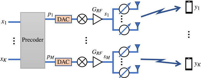
Figure 1. System model for hybrid MU-MIMO communication. The precoder is a digital beamformer at the baseband, and the RF chain and phase shifters act as an analog beamformer at the mmWave band.

Figure 1 shows a schematic of M analog beamforming networks, each of which consists of a planar array antenna with N_az × N_el elements and a total antenna gain of G_A in the broadside (BS) direction. The main beam is directed using phase shifters connected to each antenna element in the array. Each PAA selects one beam at a time to transmit information. All of the PAAs are connected to a centralized processing unit that handles the precoding scheme and selects the beams of the PAAs according to a beam selection algorithm (see Section 3.3).

Perfect channel state information (CSI) at the transmitter and receiver.

Based on Figure 1, the input-output relationship is given by

$\mathbf{y}=\mathbf{H}\mathbf{s}+\mathbf{n},(1)$

where $\mathbf{y}\in {\mathbb{C}}^{K\times 1}$ is a vector comprising the received signal at each UE receiver, $\mathbf{H}\in {\mathbb{C}}^{K\times M}$ is the downlink MU-MIMO channel matrix, $\mathbf{s}\in {\mathbb{C}}^{M\times 1}$ is the transmit signal vector after passing the PAs, and $\mathbf{n}\in {\mathbb{C}}^{K\times 1}$ is the Additive White Gaussian Noise (AWGN) vector at each UE receiver with zero means and σ_n standard deviation.

Let $\mathbf{x}\in {\mathbb{C}}^{K\times 1}$ be the transmit signal vector intended for the K UEs. The transmit signals are uncorrelated $\mathrm{E}\left\{x_k{x}_{k^{\prime }}^{*}\right\}=0$, for k ≠ k′, and satisfy the power normalization $\mathrm{E}\left\{{\left|x_k\right|}^2\right\}=1$. The operation $\mathrm{E}\left\{x\right\}$ denotes mathematical expectation of x, and x* is the complex conjugate of x. Hence, further expressing Eq. 1 as

$\mathbf{y}=\mathbf{H}\sqrt{G_{RF}}\mathbf{p}+\mathbf{n}(2)$

$=\mathbf{H}\sqrt{G_{RF}}\mathbf{W}\mathbf{x}+\mathbf{n},(3)$

where $\mathbf{p}\in {\mathbb{C}}^{M\times 1}$ is the linearly precoded transmit signal vector such that p = Wx. $\mathbf{W}\in {\mathbb{C}}^{M\times K}$ is the precoding matrix with instantaneous power normalization, $\mathrm{t}\mathrm{r}\mathrm{a}\mathrm{c}\mathrm{e}\left(\mathbf{W}{\mathbf{W}}^H\right)=1$ (Lim et al., 2015; Fatema et al., 2017). The proportionality constant G_RF ≥ 0 represents the gain of the amplifier in RF chains and is assumed to be constant across all RF chains.

This study considers two linear precoding schemes: the matched-filtering (MF) precoding and the zero-forcing (ZF) precoding. The precoding matrices are given by

$\mathbf{W}=\left\{\begin{array}{cc}\frac{{\mathbf{H}}^{†}}{{\Vert {\mathbf{H}}^{†}\Vert }_F}\hfill & \text{\hspace{0.17em}for\hspace{0.17em}}\mathrm{M}\mathrm{F}\hfill \\ \frac{{\mathbf{H}}^{†}{\left({\mathbf{H}\mathbf{H}}^{†}\right)}^{-1}}{{\Vert {\mathbf{H}}^{†}{\left({\mathbf{H}\mathbf{H}}^{†}\right)}^{-1}\Vert }_F}\hfill & \text{\hspace{0.17em}for\hspace{0.17em}}\mathrm{Z}\mathrm{F},\hfill \end{array}\right.(4)$

where the instantaneous normalization of the precoding matrix mentioned above has been applied, see Eq. 3. H^† denotes the hermitian (complex-conjugate) transpose operation on matrix H, and ‖H‖_F is the Frobenius norm of the complex matrix H. The Frobenius norm in Eq. 4 above is defined as $\Vert \mathbf{H}{\Vert }_F=\sqrt{\mathrm{t}\mathrm{r}\mathrm{a}\mathrm{c}\mathrm{e}\left(\mathbf{H}{\mathbf{H}}^H\right)}=\sqrt{{\sum }_{k=1}^K{\sum }_{m=1}^M{\left|H_{k,m}\right|}^2}$. It is worthwhile to recall that MF precoding maximizes the received signal power at the UE, while the ZF eliminates the interference at the UE. (Lim et al., 2015) shows that W is independent of G_RF. It is worth noting that the selection of MF and ZF precoding schemes in this study is based on their well-established performance characteristics and relevance for comparison. While other more advanced schemes are known, like the minimum mean square error (MMSE), these schemes enable a focused and meaningful analysis of their strengths in various deployment scenarios that is sufficient to illustrate our main points.

2.2 Figures of merit

The subsections below explain the three key performance metrics emphasized in this paper: the signal-to-interference-plus-noise ratio, radio frequency amplifier gains, and achievable sum rate.

2.2.1 Signal-to-interference-plus-noise ratio −SINR

The SINR measures the desired signal quality. It is computed in terms of the received power ratios of the desired signal to the sum of interference and noise power levels. It is used to evaluate the capacity of a wireless system.

The SINR of the kth UE in the downlink, which defines the k-th-bitstream, i.e., the kth UE throughput can be computed as (see Supplementary Appendix S1 for the derivation)

${\mathrm{S}\mathrm{I}\mathrm{N}\mathrm{R}}_k=\frac{S_k}{I_k+N_k}.(5)$

where

$S_k=G_{RF}{\left|{\mathbf{H}}_{k:}{\mathbf{W}}_{:k}\right|}^2,(6)$

is the power of the desired received signal, where H_k: denotes the kth row of the channel matrix and W_:k denotes the kth column of the precoding matrix.

$I_k=G_{RF}{\displaystyle \sum _{k^{\prime }\ne k}^K}{\left|{\mathbf{H}}_{k:}{\mathbf{W}}_{:k^{\prime }}\right|}^2(7)$

is the power of the interfering signals, where W_:k′ is the k′ − th column of the precoding matrix, and

$N_k={\sigma }_n^2,(8)$

denotes the noise power at each UE receiver, defined above and assumed to be the same for all UEs. In the analysis further below, the various parameters represented by Eqs 6–8 are evaluated. These are the SINR, the desired and interference signal power levels for a given noise power level, and maximum transmit power limitations by an array antenna. It is worth noting that the SINR depends on the deployed antenna systems and the propagation channel.

2.2.2 RF amplifier gains −G_RF

As mentioned above, the power amplification required in a PAA system is of great practical relevance. Therefore, the output power of the PAs, or more specifically, the RF amplifier gains (G_RF) are of great relevance (see Figure 1 above; Eq. S1 in Supplementary Appendix S2).

Supplementary Appendix S3 shows that SINR_k is an increasing function of G_RF, therefore the maximum value for G_RF is chosen. It is chosen such that the RF chain with the highest power of the linearly precoded transmit signal is amplified to the maximum conducted power of the PAA, i.e.,

$G_{RF}=\frac{P_{c,max}}{\underset{m=1,\dots ,M}{\mathrm{m}\mathrm{a}\mathrm{x}}{‖{\mathbf{W}}_{m:}‖}^2},(9)$

where P_c,max is the maximum conducted power of the PAA, and $‖{\mathbf{W}}_{m:}‖$ is the norm of the complex vector W_m: representing the mth row of the precoding matrix. Hence, ${‖{\mathbf{W}}_{m:}‖}^2$ represents the power of the linearly precoded transmit signal p_m, which is an element of vector p in Eq. 2 (see also Figure 2).

Figure 2

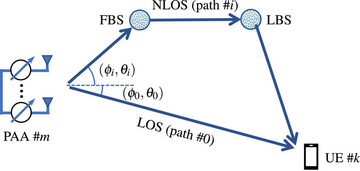
Figure 2. Illustration of multipath between PAA #m and UE #k. (ϕ_i, θ_i) represents the angle of departure of ith path.

2.2.3 Achievable sum rate −SR

To evaluate the expected system throughput that different PAAs can achieve in different propagation environments, the achievable sum-rate capacity of the M × K MIMO can be computed (Parfait et al., 2014)

$\mathrm{S}\mathrm{R}={\displaystyle \sum _{k=1}^K}{\log }_2\left(1+{\mathrm{S}\mathrm{I}\mathrm{N}\mathrm{R}}_k\right),(10)$

where SINR_k is the SINR of the kth UE computed above.

3 Propagation channel models and simulation scenarios

To establish an effective simulation environment, we focus on three crucial elements to create optimal propagation channel scenarios: channel models, the QuaDRiga channel emulator, and the beam selection algorithm.

3.1 Channel models

The propagation channel model is essential to system performance evaluation because the latter will depend on multiple propagation channel characteristics. As mentioned above, the focus is on indoor systems. In the present evaluation, well-established, standardized channel models ensure that the obtained results are relevant to the wireless community and can be easier to understand and compare to future works. Therefore, the statistical 3GPP 38.901 channel model has been used to emulate indoor office propagation channels for frequencies from 0.5–100 GHz (3GPP, 2017). For completeness, some of the main characteristics of this channel model are reproduced below.

The path gain in line-of-sight (LOS) is

$P{G}_{\mathit{LOS}}[\mathrm{d}\mathrm{B}]=-32.4-17.3{\log }_{10}\left(d_{3D}\right)-20{\log }_{10}\left(f_c\right),(11)$

where d_3D is the 3D distance in meters, and f_c is the frequency in Hz. The path gain model in non-line-of-sight (NLOS) is given by

$P{G}_{\mathit{NLOS}}[\mathrm{d}\mathrm{B}]=\min \left(P{G}_{\mathit{LOS}}[\mathrm{d}\mathrm{B}],P{G}_{\mathit{NLOS}}^{\prime }[\mathrm{d}\mathrm{B}]\right),(12)$

where

$P{G}_{\mathit{NLOS}}^{\prime }[\mathrm{d}\mathrm{B}]=-17.3-38.3{\log }_{10}\left(d_{3D}\right)-24.9{\log }_{10}\left(f_c\right).(13)$

Also, the main parameters for LOS and NLOS propagation conditions at 28 GHz are presented in Table 1. The parameters in the table include path loss exponent (PLE), shadow fading, delay spread, the azimuth angle of arrival (AoA) spread, the elevation angle of arrival (EoA) spread, the azimuth angle of departure (AoD) spread, the elevation angle of departure (EoD) spread, K-factor, cross-polarization ratio (XPR), and the number of paths (see Figure 2). In the table, μ and σ stand for mean and standard deviation, respectively.

Table 1

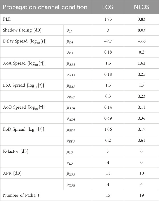
Table 1. 3GPP 38.901 channel model parameters for indoor office at 28 GHz.

The analysis will be approached in a specialized and systematic way. The considered office environments are subdivided into two main types:

• Indoor mixed office.

• Indoor open office.

These two environments are defined in (3GP, 2017). They use the 3GPP 38.901 indoor LOS and the 3GPP 38.901 indoor NLOS channels and return a LOS probability based on the 2D distance between the transmitter and the receiver. According to these models, the chance of LOS propagation in the open office is higher than in the mixed office for any distance between the transmitter and the receiver.

3.2 Channel emulation in QuaDRiGa

A structured and valuable implementation of the channel mentioned above models is available in the QuaDRiGa simulation package. QuaDRiGa can be regarded as a 3GPP 38.901 channel model reference implementation (Jaeckel et al., 2021). It incorporates full 3D propagation, including antenna modeling and scattering clusters, spherical wave propagation, and spatially correlated large and small-scale fading at both the transmitter and receiver sides of the communications link, i.e., the base station and the UE.

Figure 2 shows a sketch of the channel modeling approach in QuaDRiGa between a PAA and a UE. Given M PAAs and K UEs, the channel matrix $\tilde{\mathbf{H}}\in {\mathbb{C}}^{K\times \left(Q_{az}\times Q_{el}\right)\times M}$ represents the channel responses between all PAAs beams and UEs. Each PAA has Q_az × Q_el beams within its scanning range, where Q_az and Q_el are the number of beams in the azimuth and elevation planes, respectively. One beam per PAA is chosen based on its ability to maximize SR (see Section 3.3 for the beam selection algorithm), and H is then generated from these beams using the details described below. To compute H, the $\left(k,q,m\right)$ entry of $\tilde{\mathbf{H}}$ representing the multipath channel impulse response between the qth beam of the mth PAA and the kth UE is first computed as

${\tilde{h}}_{k,q,m}\left(t\right)={\displaystyle \sum _{i=0}^I}{h}_{i,k,q,m}^{\prime }\delta \left(t-{\tau }_i\right),(14)$

where $h_{i,k,q,m}^{\prime }$ is the impulse-response corresponding to the ith path between the mth PAA when it is beam-steered towards the qth direction, $q\in \left\{1,\dots ,Q_{az}\times Q_{el}\right\}$ and the kth UE, and τ_i is the time delay in the ith path. I + 1 is the number of channel paths: at most one LOS if it exists and I NLOS. When there is no LOS path between mth PAA and kth UE, $h_{0,k,q,m}^{\prime }$ is zero. The parameters outlined in Table 1 are utilized to determine the angles and delays associated with the ith NLOS path. Consequently, it is possible to compute the precise locations of both the first bounce scatterer (FBS) and the last bounce scatterer (LBS), referring to the initial and final reflections along the path. It is worth noting that both the radiation pattern of the PAAs and the UEs are considered in the computation of Eq. 14. For the sake of simplicity, the UE antenna radiation pattern is considered isotropic. Thus, it does not affect the channel. Finally, ${\tilde{h}}_{k,q,m}\left(t\right)$ is converted to the frequency domain to obtain ${\tilde{H}}_{k,q,m}\left(f\right)$, the $\left(k,q,m\right)$ entry of the spatial channel transfer matrix $\tilde{\mathbf{H}}$.

3.3 Beam selection for channel matrix computation

The complete channel matrix H is generated using the spatial channel transfer matrix $\tilde{\mathbf{H}}$ ((14)) in conjunction with a beam selection algorithm. In the implemented algorithm, beams maximize the MU-MIMO achievable sum-rate capacity because it is a fundamental figure of merit for a wireless system. The approach assumes an exhaustive search scheme, as suggested in (Han et al., 2017). It evaluates all the possible combinations of the beams and chooses the optimal selection. All channels from the PAAs’ beams to the UEs are assumed to be known. Each of M PAAs produces Q_az × Q_el beams, resulting in a total of ${\left(Q_{az}\times Q_{el}\right)}^M$ beam combinations. After evaluating the achievable sum-rate capacity of each combination using Eq. 10, the optimum combination can be selected

$\left(i_1,\dots ,i_M\right)=\underset{i_1,\dots ,i_M=1,\dots ,Q_{az}{Q}_{el}}{\mathrm{a}\mathrm{r}\mathrm{g}\mathrm{m}\mathrm{a}\mathrm{x}}\mathrm{S}\mathrm{R}.(15)$

This approach optimizes the performance and gives an upper bound on performance. However, the algorithm represented by Eq. 15 is time-consuming and needs to be replaced in further studies to provide more practical results.

4 Simulation scenarios and simulation steps

In this section, we detail the simulation scenarios, including both distributed and collocated deployments of phased array antennas. We also provide a flowchart that outlines all the steps involved in the simulations.

4.1 Collocated vs distributed antenna systems

As discussed above, the performance of various PAA systems is evaluated in two essentially different deployment scenarios:

• Collocated PAAs.

• Distributed PAAs.

Figure 3 depicts an aerial view of the two scenarios. In the collocated scenario, all PAAs are placed in one corner of the room next to each other. On the other hand, in the distributed deployment scenario, PAAs are placed in all four corners.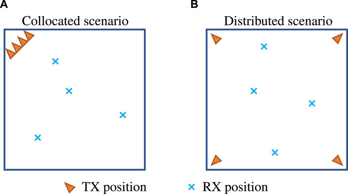

Figure 3

Figure 3. Bird’s-eye view of the simulated indoor office. (A) Collocated scenario, and (B) Distributed scenario. The TX denotes the fixed position of the BS antennas while the RX denotes a random realization of the UE positions.

Results will be specialized to an indoor environment comprising a room of 80 × 80 × 3 m³ in size. The placement heights of the PAAs and the UE antennas are 3 m and 1 m, respectively. The UE positions in the room are random in the horizontal plane with a uniform distribution. The room parameters are defined according to Table 7.2-2 in (3GP, 2017), where a detailed scenario description is provided for channel model calibration. The center-to-center distance between neighboring PAAs in collocated scenarios is set to 20 cm, and they are aligned to have the BS direction towards the center of the room.

Three antenna system simulation cases are considered for each scenario and propagation environment mentioned above, as shown in Table 2. Hereafter, the number of UEs and PAAs in all simulations is K = M = 4. Cases 1 and 2 make use of the PAA presented in (Bagheri et al., 2023b), which is capable of analog beamforming within an angular range of ±60° and ±10° in the azimuth and elevation planes, respectively. A useful feature of this PAA is that it is modular with four identical and independent subarrays. Therefore, the PAA can function in two ways: first, all subarrays form one large PAA, corresponding to Case 1, and second, each subarray works as an independent PAA, as in Case 2. Case 1 has a high antenna gain of 29.4 dBi in the BS direction. Case 2 has a lower antenna gain of 23.4 dBi in the BS direction. As a result of the high antenna gain and larger aperture in Case 1, its half-power beamwidth (HPBW) is smaller than that of Case 2. Case 3 uses a PAA with a 23.1 dBi antenna gain in the BS direction (Bagheri et al., 2023a). This PAA can only beamform in the azimuth plane within an angular range of ±60°. The beam coverage of the PAAs is shown in Figure 4, where the antenna gain by the PAAs in the main beams at each angle $\left[Q_{az},Q_{el}\right]$ is shown.

Table 2

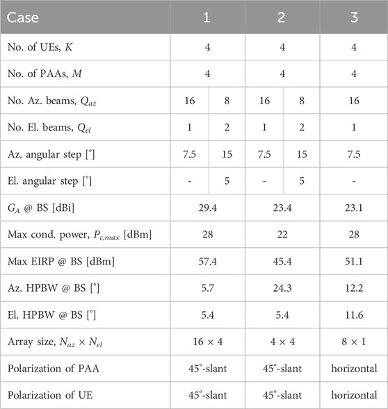
Table 2. Parameters of the three antenna system simulation cases based on two different state-of-the-art mmWave PAA Bagheri et al. (2023a), Bagheri et al. (2023b).

Figure 4

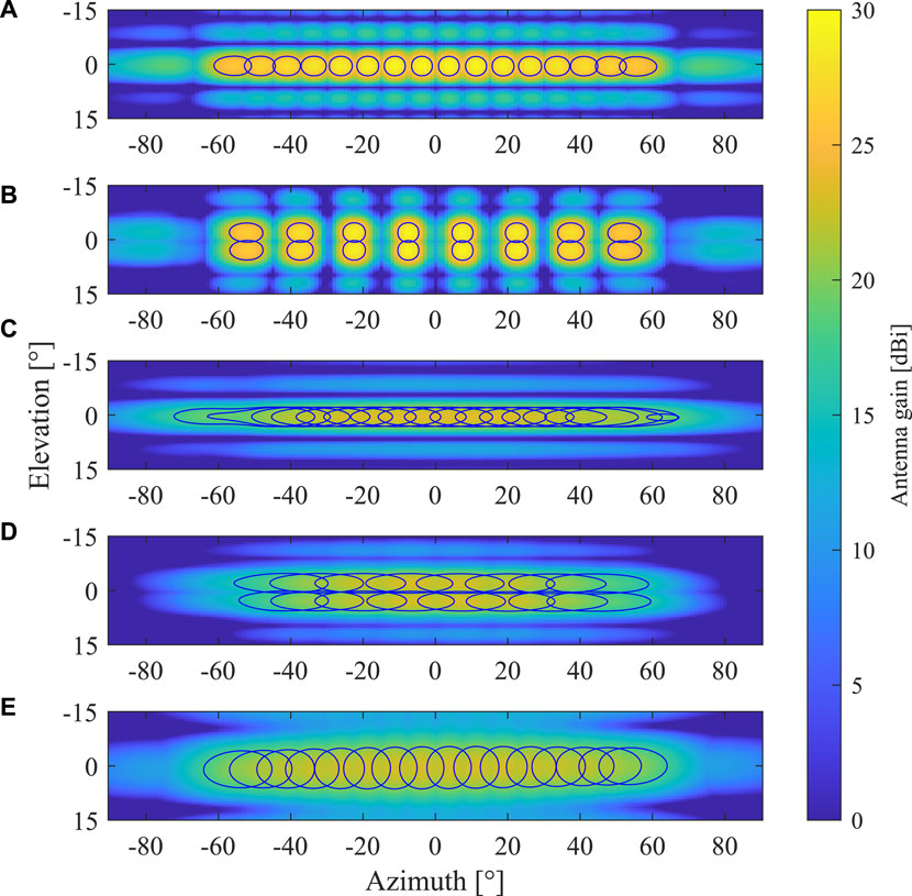
Figure 4. The beam coverage of PAAs, when all the possible beams are combined. (A) Case 1 with $\left[Q_{az},Q_{el}\right]=\left[\mathrm{16,1}\right]$, (B) Case 1 with $\left[Q_{az},Q_{el}\right]=\left[\mathrm{8,2}\right]$, (C) Case 2 with $\left[Q_{az},Q_{el}\right]=\left[\mathrm{16,1}\right]$, (D) Case 2 with $\left[Q_{az},Q_{el}\right]=\left[\mathrm{8,2}\right]$, and (E) Case 3, where $\left[Q_{az},Q_{el}\right]=\left[\mathrm{16,1}\right]$. Overlaid are the 3 dB contours of the beams.

Another important property of PAAs is effective isotropic radiated power (EIRP), which is defined as

$\mathrm{E}\mathrm{I}\mathrm{R}\mathrm{P}=P_c{G}_A,(16)$

where P_c is the conducted power and G_A is the total array antenna gain. Using Eq. 16 above and Eq. S2 in Supplementary Appendix S2, EIRP for each PAA in Figure 1 can be written as

$\begin{array}{cc}\hfill {\mathrm{E}\mathrm{I}\mathrm{R}\mathrm{P}}_m& =\mathrm{E}\left\{{\left|s_m\right|}^2\right\}{G}_{A_m}\hfill \\ \hfill & =G_{RF}{‖{\mathbf{W}}_{m:}‖}^2{G}_{A_m}.\hfill \end{array}(17)$

Therefore, the EIRP of the PAAs as given by Eq. 17 is limited by G_RF and total array antenna gain $({\mathrm{E}\mathrm{I}\mathrm{R}\mathrm{P}}_m<G_{RF}{G}_{A_m})$. The maximum EIRP values for the PAAs considered here are 9 dB backed off from their saturation points to preserve signal linearity. The simulations use these EIRP values with the conducted powers P_c. The maximum conducted power P_c,max is chosen to meet the maximum total radiated power (TRP) for local area base stations of 33 dBm (3GPP,2018).

4.2 Simulation steps

A concise flow chart of the main simulation steps is shown in Figure 5. The structure follows the modeling approach outlined above, including the computation of the figures of merit of interest.

Figure 5

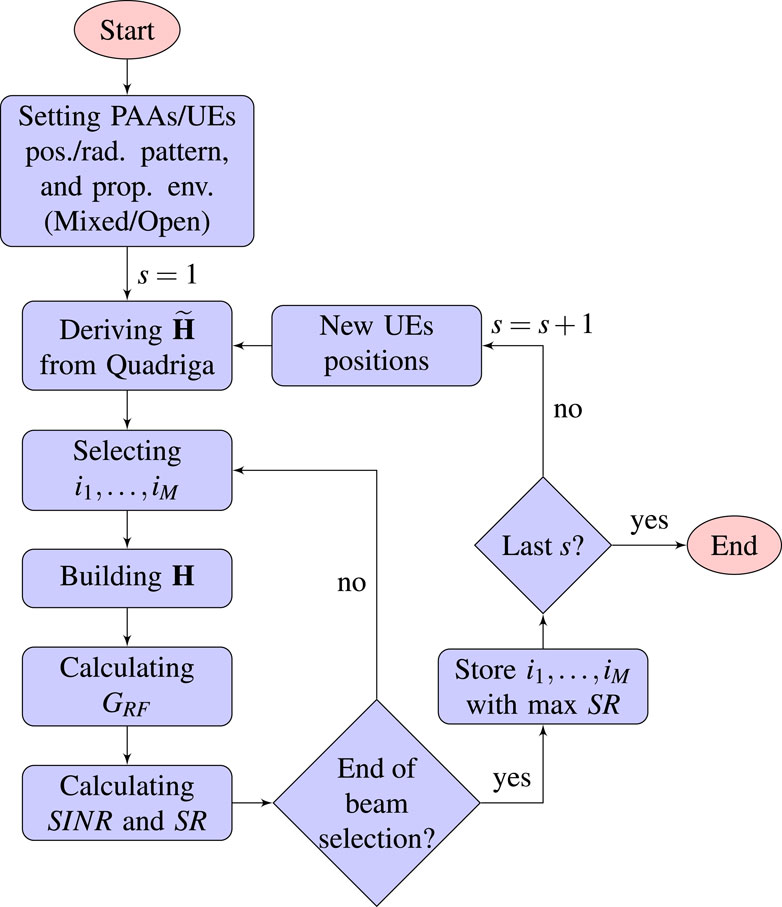
Figure 5. Flow chart of the simulation steps.

The simulation study compares the deployment of two different PAAs, realized in fundamentally two different spatial configurations of the PAAs in two different indoor propagation environments, and evaluated for two different beamforming algorithms.

The operational frequency chosen for the simulations is 28 GHz. The noise power and interference level play essential roles in the quality of the received signal. Here and for the rest of the paper, the noise power at the UEs is ${\sigma }_n^2=N_{0}B=-99$ dBm, where N₀ = −174 dBm/Hz is the thermal noise power in a 1-Hz bandwidth at room temperature and B = 30 MHz is the signal bandwidth. The total number of samples for a single simulation is 500; hence, s = 1, …, 500. All computed parameters are shown as empirical cumulative distribution functions (CDFs). Corresponding mean values and standard deviations are also computed. For G_RF, the received signal, interference, and SINR, mean and standard deviation values are computed in the logarithmic domain. This is due to the log-normal distribution of these parameters in downlink cellular networks (Hadj-Kacem et al., 2020).

5 Simulation results and analysis

This section showcases the simulation results and discusses our key findings and observations.

5.1 Path gain

To illustrate the impact of the propagation channels on the received signals when beamforming is employed, the received signal has been computed at several positions evenly distributed over the simulated room for two different propagation channels. Figure 6 shows the distribution of the link path gain plus antenna gain (in dB) for the PAAs in all cases based on the corresponding Eqs 11–13 given above. Results are shown when the arrays transmit in the BS direction. Two propagation channels are considered:

Figure 6

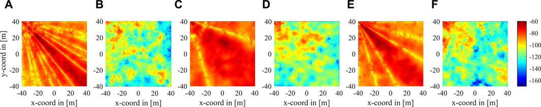
Figure 6. The distribution of the path gain plus antenna gain (in dB) in two propagation conditions and three antenna system simulation cases. (A) Case 1 in the 3GPP 38.901 indoor LOS channel, (B) Case 1 in the 3GPP 38.901 indoor NLOS channel, (C) Case 2 in the 3GPP 38.901 indoor LOS channel, (D) Case 2 in the 3GPP 38.901 indoor NLOS channel, (E) Case 3 in the 3GPP 38.901 indoor LOS channel, and (F) Case 3 in the 3GPP 38.901 indoor NLOS channel.

• The 3GPP 38.901 indoor LOS channel.

• The 3GPP 38.901 indoor NLOS channel.

The path gains in these cases are spatially correlated. The effects of the main lobe, side lobes, and nulls of the antenna’s radiation pattern are visible in Figures 6A,C,E. Multipath propagation has changed the path gain distribution considerably. As a result, the gain has increased at some positions, more visibly in the direction of pattern nulls. The distribution of the received signal has become more even. In Figures 6B,D,F, the effect of the radiation pattern is not visible anymore, and the values of the path gain plus antenna gain have dropped significantly. Computing the average path gain in linear scale over all the simulated room positions gives the following values in dB scale: −75.5, −100.6, −75.2, −96.7, −75.6. These values correspond to Figure 6A through F. These average values are well correlated with the respective PLEs. As seen from the above results, the propagation channel behaves differently in different environments, which may negatively impact the system performance, as evaluated next. Moreover, as multipath propagation becomes predominant, digital beamforming that adapts the communication link to the spatially selective channel becomes more relevant. The optimized performance might be achieved through the scatters, i.e., the environment, instead of forming a well defined beam towards the users.

5.2 RF PA gains

The CDFs of RF power amplifier gains G_RF Eq. 9 of all PAAs (see Supplementary Appendix S2) are shown in Figure 7 for Case 1 (see Table 2). The other two cases are omitted because the main shapes are the same. On the other hand, the mean value and standard deviation corresponding to computed CDFs for all three cases are presented in Table 3.

Figure 7

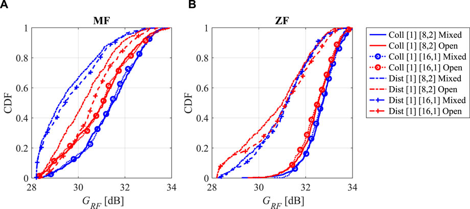
Figure 7. The CDFs of G_RF in Case 1: (A) MF and (B) ZF. See Table 2 for the parameters of the three antenna system simulation cases.

Table 3

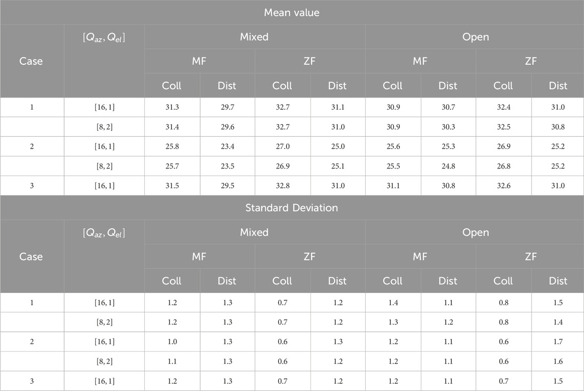
Table 3. Mean value and standard deviation of G_RF [dB]. See Table 2 for the parameters of the three antenna system simulation cases.

It can be seen from Table 3 that the PAA distributed deployment scenario (Dist.) requires lower G_RF than the collocated scenario (Coll.) regardless of the propagation scenario, the precoding scheme, and the antennas and beams used. The required power is on the order of $\approx 1.45$ dB lower on average, i.e., about 40% lower power amplifier (PA) gain needed across all cases. The computed G_RF difference in dB between the Dist. scenario and the Coll. scenario in the mixed environment varies from 1.6–2.4 dB (45–74%), observed across all the cases and precoding algorithms. In contrast, in the open propagation environment, it goes from 0.2–1.7 dB (5–48%). A similar comparison shows that for the MF precoding, the reduction is from 0.2–2.4 dB (5–74%), and for the ZF precoding, it is from 1.6–2.0 dB (45–58%), observed across the propagation environments and cases.

As can be seen above, the choice of precoding scheme affects the PA gains G_RF, too. Looking at Table 3, it becomes apparent that, indeed, ZF requires, in general, a higher G_RF than MF. This is expected because MF is well-known to optimize the link power while ZF minimizes interference. The MF requires $\approx 1.11$ dB (29%) less power than the ZF, regardless of the propagation scenario, the antennas and beams used, and the deployment scenario (i.e., Coll. or Dist.). More specifically, comparing the reduction of G_RF with MF compared to the ZF precoding in the mixed scenario is from 1.2–1.6 dB (32–45%), while it is from −0.1 − 1.6 dB (−2 − 45%) in the open propagation scenario. It is worth reminding that the negative values −0.1 dB (−2) % indicate an increase rather than a decrease, which was observed for only one of the twenty possible simulated instances, i.e., for Case 2 [16,1] open propagation scenario.

The reduction of G_RF depends on the propagation environment, the antenna type, and the deployment scenario, as illustrated above. As shown in Table 2, Case 1 and 3, having the same P_c,max, use an equal amount of RF power. Case 2 transmits roughly 6 dB (300%) less than the other cases, with 6 dB less P_c,max as well. On the other hand, the spatial beam arrangement of each PAA $(\left[Q_{az},Q_{el}\right])$ shows no significant change in the total conducted RF transmit power. In this context, the most significant reduction of G_RF is for Case 2 with $\left[\mathrm{16,1}\right]$ and $\left[\mathrm{8,2}\right]$ beams using MF precoding in the mixed propagation environment.

Regarding the standard deviation, it can be seen from Table 3 that it remains almost unchanged across Cases 1, 2, and 3 and that the values are relatively low. There is an increment when using distributed antennas compared to collocated for most considered instances, but the MF precoding in the open space propagation scenario. The latter might be explained by the fact that it becomes more likely to be in a focused beam with slight channel variation.

5.3 SINR

The SINRs at the UE locations are computed using Eq. 5 and are shown in Figure 8 for Case 1 only because of the same reasons as above. Table 4 shows the mean value and standard deviation.

Figure 8

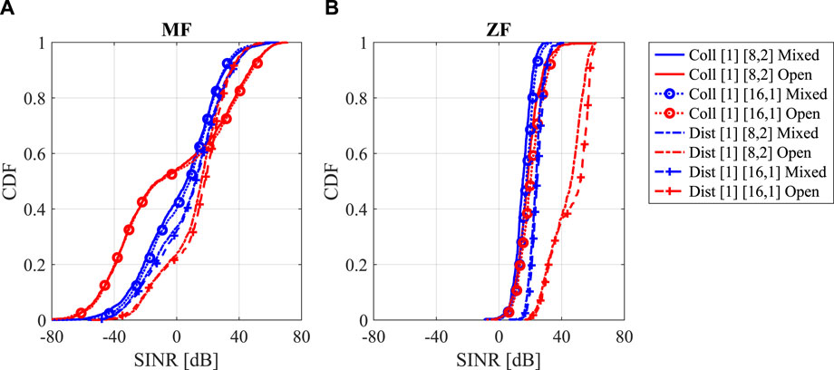
Figure 8. The CDFs of SINR at the UE locations in Case 1: (A) MF, and (B) ZF. See Table 2 for the parameters of the three antenna system simulation cases.

Table 4

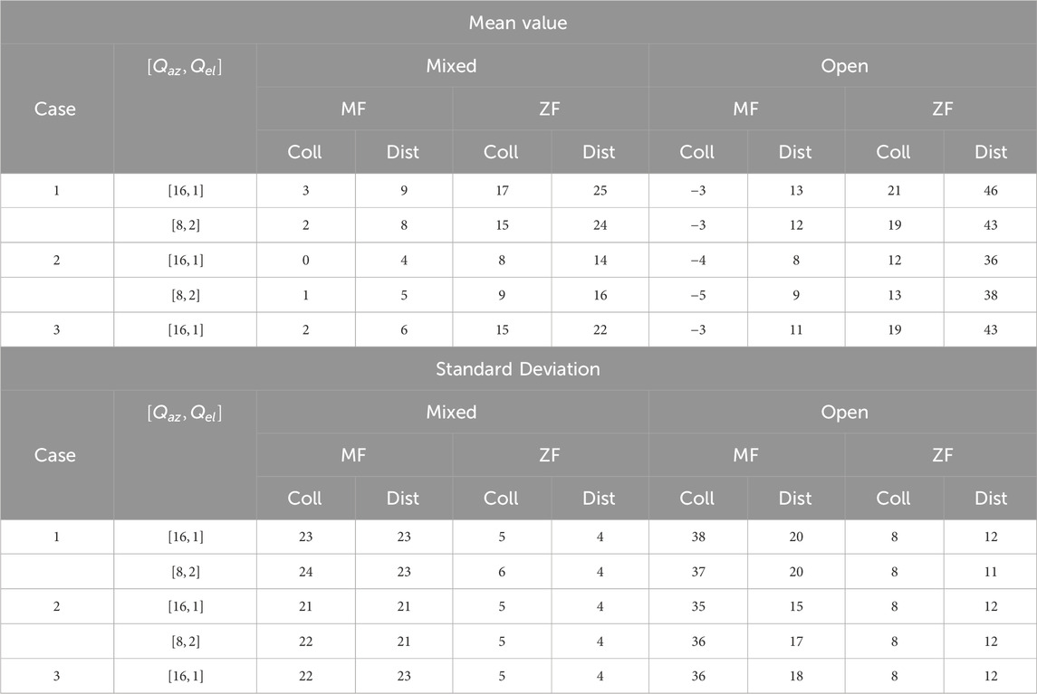
Table 4. Mean value and standard deviation of SINR [dB]. See Table 2 for the parameters of the three antenna system simulation cases.

As seen from Table 4, the SINR increases with deploying distributed antennas compared to collocation with an average of 12.7 dB, as seen across all the results. The SINR increment is larger in the open propagation environment with an average of 19.3 dB compared to 6.1 dB in the mixed environment computed over all the cases and precoding schemes.

Furthermore, on average, the SINR with ZF is 19 dB higher than with MF computed over all the propagation scenarios and cases. In the open propagation environment, the average SINR increase is 25.5 dB compared to 12.5 dB in the mixed propagation environment. It should be noted here that ZF precoding produces a SINR distribution with a lower standard deviation than MF. This gives the benefit of a more reliable link between PAAs and UEs.

The signal power by UEs also increases when the PAAs are distributed in all cases. This is due to the higher path gain in the distributed deployment scenario. In addition, the standard deviation of the received signal power decreases when PAAs are distributed. The LOS probability is higher in the open propagation environment; therefore, the received signal level also generally increases. Almost always, in the distributed deployment scenario in the open propagation environment, the UEs are within LOS distance of at least one PAA. Still, in the collocated scenario, there is a high probability that the UEs do not see any PAA in their LOS. While not shown here, it was observed that the mean of the received signal level in the distributed deployment of the open propagation environment is $\approx 20$ dB higher than the mixed environment.

The most significant increase of SINR is for Case 1 with $\left[\mathrm{16,1}\right]$ and $\left[\mathrm{8,2}\right]$ beams using ZF precoding in the open propagation environment.

As in the case of the PA gains above, the variability is similar for the antenna types and beam configurations. As seen from Table 4, the ZF precoding has a much lesser standard deviation than the MF precoding. Moreover, the standard deviation is larger in the open propagation environment than in the mixed environment. The comparison of distributed versus collocated is less straightforward and depends on the case.

5.4 Achievable SR

Figure 9 shows the CDF of the achievable sum rate computed by Eq. 10 for Case 1. All the curves have been obtained from 500 simulated data points, i.e., channel realizations. Table 5 summarizes the simulations’ mean value and standard deviation.

Figure 9

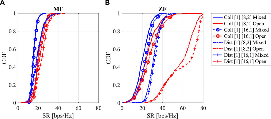
Figure 9. The CDFs of achievable sum-rate capacity in Case 1: (A) MF and (B) ZF. See Table 2 for the parameters of the three antenna system simulation cases.

Table 5

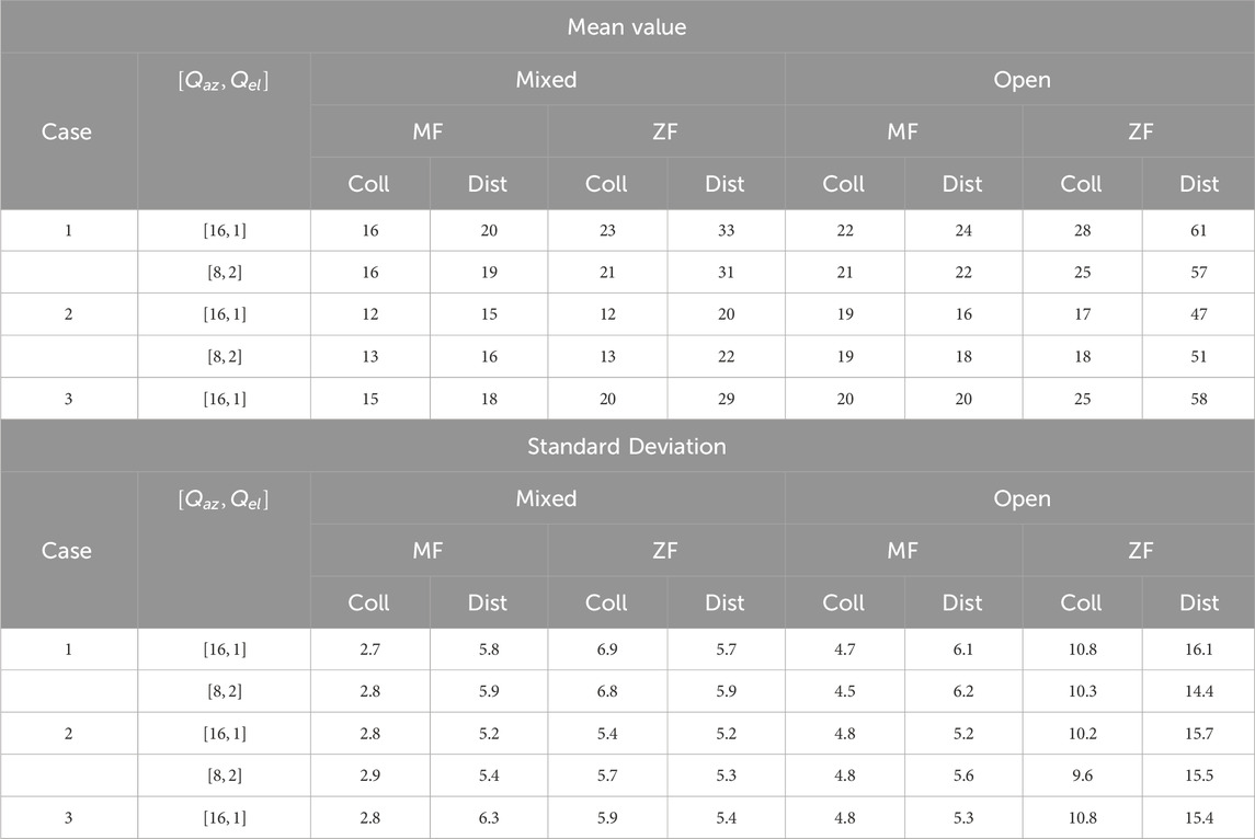
Table 5. Mean value and standard deviation of SR [bps/Hz]. See Table 2 for the parameters of the three antenna system simulation cases.

It can be immediately seen from the shown results that the distributed deployment scenario always leads to higher SR because of the similar behavior of the SINR. On average, the SR in the distributed deployment scenario is 11.1 bps/Hz larger than in the collocated scenario for all the propagation scenarios, cases, and precoding schemes. The numbers in open and mixed propagation environments are 16 bps/Hz and 6.2 bps/Hz, respectively. The distribution of PAAs increases the chance for UEs to make a LOS link with at least one PAA in the open propagation environment.

The ZF precoding shows a larger SR increase than the MF precoding. It is mainly because ZF removes the interference at UE positions. On average, ZF SR is 12.5 bps/Hz larger than the MF for all the cases and propagation environments. The corresponding improvements in the open and mixed environments are 18.5 bps/Hz and 6.4 bps/Hz, respectively, because of the higher LOS probability.

The largest SR are observed for both scenarios of Case 1 when $\left[\mathrm{16,1}\right]$ and $\left[\mathrm{8,2}\right]$. Since the vertical spread of the UE locations in the indoor environment is limited, it is advantageous that all of the beams are in the same plane when the HPBW is small—with $\left[\mathrm{16,1}\right]$ beams covering the azimuth plane within their HPBW (look at Figures 4A,B). Meanwhile, the opposite effect can be seen in both scenarios of Case 2, where beams with larger HPBW are employed. When $\left[\mathrm{8,2}\right]$ beams are used, SR increases in both collocated and distributed deployment scenarios. Figures 4C,D show the beam coverage by the antenna of Case 2.

In terms of the standard deviation of the sum-rate capacity, it can be see from Table 5 that it is larger for the ZF precoding employed in a distributed antenna scenario than for the MF in a collocated scenario. Moreover, the standard deviation is larger in the open environment than in the mixed environment. As in the case of the power amplifier gain and the SINR, the standard deviation is relatively stable across the antenna types and beam configurations.

Table 6 overviews the top four simulation instances, ranked according to the SR mean in 3GPP-defined indoor mixed and open propagation environments. The table also shows the SR values corresponding to a CDF probability level equal to 0.05, denoted as CDF_SR = 0.05 in the table. As established above, PAA distributed deployment scenarios consistently perform better than collocated scenarios. In addition, the ZF precoding scheme offers a higher average achievable SR capacity due to a higher SINR. At the same time, a lower PA gain is needed in distributed than collocated scenarios, as established above. Also, when comparing the ZF precoding in the indoor scenarios, a higher SR can be expected from the open propagation environment than the mixed propagation environment. We believe it is mainly due to the higher probability of the LOS condition.

Table 6

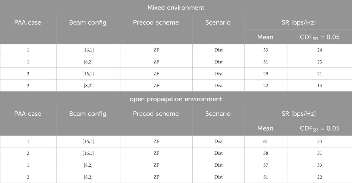
Table 6. The scenarios with the best performance are sorted by the mean SR. See Table 2 for the parameters of the three antenna system simulation cases.

6 Conclusion

This paper evaluates three antenna system cases based on two 28 GHz phased array antennas (PAAs). Hybrid digital-analog multi-beam communications in indoor scenarios were studied following the 3GPP 38.901 standard channel models. The study involves PAAs designed for mmWave 5G communication, investigating their performance in two setups: collocated and distributed PAA systems, azimuth-only $\left[\mathrm{16,1}\right]$ beams, elevation-azimuth $\left[\mathrm{8,2}\right]$ beams, two digital precoding schemes, i.e., matched filter and zero-forcing, and two indoor propagation environments, i.e., mixed and open.

Based on our study, we can conclude that the distributed hybrid digital-analog multi-beam systems prove to be a highly effective strategy for enhancing achievable capacity. This conclusion is supported by several significant findings: a substantial increase in data capacity ranging from 117% to 183% compared to collocated deployment, a notable reduction in power amplifier gain by 38%–51%, resulting in improved power efficiency, and the optimization of system performance through tailored analog beam configurations. The study underscores the effectiveness of the zero-forcing precoding scheme, particularly in high-power setups, and highlights the superiority of line-of-sight propagation in open spaces over mixed indoor environments. The identified optimal configurations for large phased array antennas (PAAs) comprised 16 × 4 elements with azimuth-only $\left[\mathrm{16,1}\right]$ beams, and ZF precoding stands out as the absolute gain leader. On the other hand, compact PAAs featuring 4 × 4 elements with elevation-azimuth $\left[\mathrm{8,2}\right]$ beams achieve the largest relative gain. In summary, distributed hybrid digital-analog multi-beam systems present a robust and efficient solution, offering substantial gains in data capacity while concurrently reducing power consumption.

Selecting a phased array antenna (PAA) for indoor wireless communication involves numerous parameters. While high Equivalent Isotropically Radiated Power (EIRP) is essential, achieving high-data-rate communication requires additional conditions. Future work could incorporate a more practical beam selection algorithm and optimize per-antenna power gain. Further research might explore advanced techniques, e.g., based on the minimum mean square error (MMSE) scheme, balancing the trade-off between maximizing desired signal power and minimizing interference under varying channel conditions. Scalability experiments considering the number of users and antenna system size could offer additional insights. In a broader context, future work might examine how altering system parameters affects key findings, contributing to a deeper understanding of beamforming strategies in 5G systems for enhanced efficiency and performance.

Data availability statement

The raw data supporting the conclusion of this article will be made available by the authors, without undue reservation.

Author contributions

AB: Formal Analysis, Investigation, Methodology, Visualization, Writing–original draft, Writing–review and editing. CB: Supervision, Writing–review and editing. AG Methodology, Supervision, Writing–review and editing, Conceptualization, Formal Analysis, Funding acquisition, Project administration, Writing–original draft.

Funding

The author(s) declare financial support was received for the research, authorship, and/or publication of this article. This work was partly supported by European Union Horizon 2020 research and innovation program under the Marie Skłodowska-Curie grant agreement No. 766231 WAVECOMBE H2020-MSCA-ITN-2017. Funding from the ELLIIT strategic research environment (https://elliit.se/) is also appreciated.

Conflict of interest

Authors AB and CB were employed by Gapwaves AB.

The remaining author declares that the research was conducted in the absence of any commercial or financial relationships that could be construed as a potential conflict of interest.

The author(s) declared that they were an editorial board member of Frontiers, at the time of submission. This had no impact on the peer review process and the final decision

Publisher’s note

All claims expressed in this article are solely those of the authors and do not necessarily represent those of their affiliated organizations, or those of the publisher, the editors and the reviewers. Any product that may be evaluated in this article, or claim that may be made by its manufacturer, is not guaranteed or endorsed by the publisher.

Supplementary material

The Supplementary Material for this article can be found online at: https://www.frontiersin.org/articles/10.3389/frcmn.2024.1354628/full#supplementary-material

References

3GPP (2017). Study on channel model for frequencies from 0.5 to 100 GHz. Tech. Rep. TR 38. 901 V14.1.0, 3rd Generation Partnership Project.

Google Scholar

3GPP (2018). 5G NR Base Station (BS) radio transmission and reception. Tech. Rep. Tr. 38, 104. V15.3.0, 3rd Generation Partnership Project.

Google Scholar

Akbar, N., Björnson, E., Larsson, E. G., and Yang, N. (2018). “Downlink power control in massive MIMO networks with distributed antenna arrays,” in 2018 IEEE International Conference on Communications (ICC), Kansas City, MO, USA, 20-24 May 2018 (IEEE), 1–6.

CrossRef Full Text | Google Scholar

Arnold, M., Baracca, P., Wild, T., Schaich, F., and ten Brink, S. (2021). “Measured distributed vs co-located massive MIMO in industry 4.0 environments,” in 2021 Joint European Conference on Networks and Communications & 6G Summit (EuCNC/6G Summit), Porto, Portugal, 08-11 June 2021 (IEEE), 306–310.

CrossRef Full Text | Google Scholar

Bagheri, A., Bencivenni, C., Gustafsson, M., and Glazunov, A. A. (2023a). A 28 GHz 8 × 8 gapwaveguide phased array employing GaN front-end with 60 dBm EIRP. IEEE Trans. Antennas Propag. 71, 4510–4515. doi:10.1109/tap.2023.3240837

CrossRef Full Text | Google Scholar

Bagheri, A., Karlsson, H., Bencivenni, C., Gustafsson, M., Emanuelsson, T., Hasselblad, M., et al. (2023b). A 16 × 16 45° slant-polarized gapwaveguide phased array with 65-dBm EIRP at 28 GHz. IEEE Trans. Antennas Propag. 71, 1319–1329. doi:10.1109/tap.2022.3227718

CrossRef Full Text | Google Scholar

Bjornson, E., Van der Perre, L., Buzzi, S., and Larsson, E. G. (2019). Massive MIMO in sub-6 GHz and mmWave: physical, practical, and use-case differences. IEEE Wirel. Commun. 26, 100–108. doi:10.1109/mwc.2018.1800140

CrossRef Full Text | Google Scholar

Chen, C.-M., Guevara, A. P., and Pollin, S. (2017). “Scaling up distributed massive MIMO: why and how,” in 2017 51st Asilomar Conference on Signals, Systems, and Computers, Pacific Grove, CA, USA, 29 October 2017 - 01 November 2017 (IEEE), 271–276.

CrossRef Full Text | Google Scholar

Choi, T., Luo, P., Ramesh, A., and Molisch, A. F. (2020). “Co-located vs distributed vs semi-distributed MIMO: measurement-based evaluation,” in 2020 54th Asilomar Conference on Signals, Systems, and Computers, Pacific Grove, CA, USA, 01-04 November 2020 (IEEE), 836–841.

CrossRef Full Text | Google Scholar

Elhoushy, S., and Hamouda, W. (2020). Performance of distributed massive MIMO and small-cell systems under hardware and channel impairments. IEEE Trans. Veh. Technol. 69, 8627–8642. doi:10.1109/tvt.2020.2998405

CrossRef Full Text | Google Scholar

Fatema, N., Hua, G., Xiang, Y., Peng, D., and Natgunanathan, I. (2017). Massive MIMO linear precoding: a survey. IEEE Syst. J. 12, 3920–3931. doi:10.1109/jsyst.2017.2776401

CrossRef Full Text | Google Scholar

Ghosh, A., Thomas, T. A., Cudak, M. C., Ratasuk, R., Moorut, P., Vook, F. W., et al. (2014). Millimeter-wave enhanced local area systems: a high-data-rate approach for future wireless networks. IEEE J. Sel. Areas Commun. 32, 1152–1163. doi:10.1109/jsac.2014.2328111

CrossRef Full Text | Google Scholar

Hadj-Kacem, I., Braham, H., and Jemaa, S. B. (2020). SINR and rate distributions for downlink cellular networks. IEEE Trans. Wirel. Commun. 19, 4604–4616. doi:10.1109/twc.2020.2985681

CrossRef Full Text | Google Scholar

Han, Y., Jin, S., Zhang, J., Zhang, J., and Wong, K.-K. (2017). “Analog beam selection schemes of DFT-based hybrid beamforming multiuser systems,” in 2017 23rd Asia-Pacific Conference on Communications (APCC), Perth, WA, Australia, 11-13 December 2017 (IEEE), 1–6.

CrossRef Full Text | Google Scholar

Islam, S. F. (2022) Distributed massive MIMO in millimetre wave communication. University of York. Ph.D. thesis.

Google Scholar

Jaeckel, S., Raschkowski, L., Börner, K., and Thiele, L. (2014). QuaDRiGa: a 3-D multi-cell channel model with time evolution for enabling virtual field trials. IEEE Trans. Antennas Propag. 62, 3242–3256. doi:10.1109/tap.2014.2310220

CrossRef Full Text | Google Scholar

Jaeckel, S., Raschkowski, L., Börner, K., Thiele, L., Burkhardt, F., and Eberlein, E. (2021). QuaDRiGa - quasi deterministic radio channel generator, user manual and documentation. Tech. Rep. V2 (6). Fraunhofer Heinrich Hertz Institute.

Google Scholar

Jeong, S., Farhang, A., Gao, F., and Flanagan, M. F. (2020). Frequency synchronisation for massive MIMO: a survey. IET Commun. 14, 2639–2645. doi:10.1049/iet-com.2019.1291

CrossRef Full Text | Google Scholar

Kamga, G. N., Xia, M., and Aïssa, S. (2016). Spectral-efficiency analysis of massive MIMO systems in centralized and distributed schemes. IEEE Trans. Commun. 64, 1930–1941. doi:10.1109/tcomm.2016.2519513

CrossRef Full Text | Google Scholar

Kim, J., Sung, M., Cho, S.-H., Won, Y.-J., Lim, B.-C., Pyun, S.-Y., et al. (2019). MIMO-supporting radio-over-fiber system and its application in mmWave-based indoor 5G mobile network. J. Light. Technol. 38, 101–111. doi:10.1109/jlt.2019.2931318

CrossRef Full Text | Google Scholar

Lim, Y.-G., Chae, C.-B., and Caire, G. (2015). Performance analysis of massive MIMO for cell-boundary users. IEEE Trans. Wirel. Commun. 14, 6827–6842. doi:10.1109/twc.2015.2460751

CrossRef Full Text | Google Scholar

Marzetta, T. L. (2010). Noncooperative cellular wireless with unlimited numbers of base station antennas. IEEE Trans. Wirel. Commun. 9, 3590–3600. doi:10.1109/twc.2010.092810.091092

CrossRef Full Text | Google Scholar

Parfait, T., Kuang, Y., and Jerry, K. (2014). “Performance analysis and comparison of ZF and MRT based downlink massive MIMO systems,” in 2014 Sixth International Conference on Ubiquitous and Future Networks (ICUFN), Shanghai, China, 08-11 July 2014 (IEEE), 383–388.

CrossRef Full Text | Google Scholar

Pérez, J. R., Fernández, Ó., Valle, L., Bedoui, A., Et-tolba, M., and Torres, R. P. (2021). Experimental analysis of concentrated versus distributed massive MIMO in an indoor cell at 3.5 GHz. Electronics 10, 1646. doi:10.3390/electronics10141646

CrossRef Full Text | Google Scholar

Rangan, S., Rappaport, T. S., and Erkip, E. (2014). Millimeter-wave cellular wireless networks: potentials and challenges. Proc. IEEE 102, 366–385. doi:10.1109/jproc.2014.2299397

CrossRef Full Text | Google Scholar

Rusek, F., Persson, D., Lau, B. K., Larsson, E. G., Marzetta, T. L., Edfors, O., et al. (2012). Scaling up MIMO: opportunities and challenges with very large arrays. IEEE Signal Process. Mag. 30, 40–60. doi:10.1109/msp.2011.2178495

CrossRef Full Text | Google Scholar

Sheng, N., Zhang, J., Zhang, F., and Tian, L. (2011). “Downlink performance of indoor distributed antenna systems based on wideband MIMO measurement at 5.25 GHz,” in 2011 IEEE Vehicular Technology Conference (VTC Fall), San Francisco, CA, USA, 05-08 September 2011 (IEEE), 1–5.

CrossRef Full Text | Google Scholar

Van, S. D., Ngo, H. Q., and Cotton, S. L. (2020). Wireless powered wearables using distributed massive MIMO. IEEE Trans. Commun. 68, 2156–2172. doi:10.1109/tcomm.2020.2965442

CrossRef Full Text | Google Scholar

Wang, C.-X., Haider, F., Gao, X., You, X.-H., Yang, Y., Yuan, D., et al. (2014). Cellular architecture and key technologies for 5G wireless communication networks. IEEE Commun. Mag. 52, 122–130. doi:10.1109/mcom.2014.6736752

CrossRef Full Text | Google Scholar

Wang, D., Wang, J., You, X., Wang, Y., Chen, M., and Hou, X. (2013). Spectral efficiency of distributed MIMO systems. IEEE J. Sel. Areas Commun. 31, 2112–2127. doi:10.1109/jsac.2013.131012

CrossRef Full Text | Google Scholar

Xiao, M., Mumtaz, S., Huang, Y., Dai, L., Li, Y., Matthaiou, M., et al. (2017). Millimeter wave communications for future mobile networks. IEEE J. Sel. Areas Commun. 35, 1909–1935. doi:10.1109/jsac.2017.2719924

CrossRef Full Text | Google Scholar

You, X.-H., Wang, D.-M., Sheng, B., Gao, X.-Q., Zhao, X.-S., and Chen, M. (2010). Cooperative distributed antenna systems for mobile communications [coordinated and distributed MIMO]. IEEE Wirel. Commun. 17, 35–43. doi:10.1109/mwc.2010.5490977

CrossRef Full Text | Google Scholar

Yue, D.-W., and Nguyen, H. H. (2019). Multiplexing gain analysis of mmWave massive MIMO systems with distributed antenna subarrays. IEEE Trans. Veh. Technol. 68, 11368–11373. doi:10.1109/tvt.2019.2943663

CrossRef Full Text | Google Scholar

Zhu, Y.-H., Callebaut, G., Çalık, H., Van der Perre, L., and Rottenberg, F. (2022). Energy efficient access point placement for distributed massive MIMO. Network 2, 288–310. doi:10.3390/network2020019

CrossRef Full Text | Google Scholar