Multi-Scale Process Monitoring Based on Time-Frequency Analysis and Feature Fusion

Data-driven process monitoring is an important tool to ensure safe production and smooth operation. Generally, implicit information can be mined through data processing and analysis algorithms to detect process disturbances on the basis of historical production data. In industrial practice, signals with different sources of disturbance show different distribution patterns along with the time domain and frequency domain, that is, noise and pulse-type changes are usually contained in the high-frequency portion while most process dynamic is contained in the low-frequency portion. However, feature extraction is usually implemented at a single scale in traditional multivariate statistical algorithms. With this concern, a novel multi-scale process monitoring method is proposed in this work, by which wavelet packet decomposition is first employed for time-frequency analysis. After decomposition, multivariate statistical models are established for each scale to construct process statistics. For the high-frequency part, the classical principal component analysis (PCA) algorithm is adopted to construct squared prediction error (SPE) and Hotelling $T^2\left(T^2\right)$ statistics. While for the low-frequency part, the slow feature analysis (SFA) algorithm is adopted to construct $T^2, T_{e^2}, S^2$ and $S_{e^2}$ statistics for the extraction of the long-term slowly changing trend. Then the monitoring statistics, obtained from each method at different scales, are integrated by a support vector data description (SVDD) method to give a final fault detection decision. The performance of the proposed method is verified on the benchmark Tennessee Eastman Process (TEP) and an industrial continuous catalytic reforming heat exchange unit by comparing with related multivariate statistical methods, which only focus on a single scale.

1 Introduction

The strict requirement for production safety and operation smoothness in modern chemical industry has posed high expectations for real-time process monitoring (Severson et al., 2016). In the era of industry 4.0, signal analysis and data mining technologies have experienced rapid progress and application (Ghobakhloo, 2020). Under this background, the development of data-driven process monitoring methods has attracted great attention in both academia and industry (Qin, 2012; Yin et al., 2014).

Multivariate statistical methods are developed by projecting high-dimensional data into low-dimensional feature spaces, and then statistics reflecting data features are constructed in each space for monitoring. Several multivariate statistical algorithms, including principal component analysis (PCA) (Wold et al., 1987), partial least square (PLS) (Geladi and Kowalski., 1986), independent component analysis (ICA) (Comon, 1994) and canonical correlation analysis (CCA) (Hardoon et al., 2004), have been successfully utilized to industry application. These algorithms are developed on the basis of different assumptions and suitable for the extraction of different data features. Specifically, PCA has been widely applied to the analysis of correlations between variables and has a good performance in dimension reduction of multivariate samples (Choqueuse et al., 2011). The data under normal conditions are projected into the principal subspace and residual subspace through orthogonal transformation. Then the statistics of squared prediction error (SPE) and Hotelling $T^2\left(T^2\right)$ are constructed to determine the alarm threshold. ICA is an effective algorithm for blind source signal separation (Jutten and Karhunen, 2004). A non-orthogonal transformation is performed on the original data so that the signal components are mutually independent. CCA is an effective algorithm to comprehensively consider the relationship between input variables and output variables. However, if these classic multivariate statistical methods are directly adopted to actual operation data, the real signals may be buried by noise, thus leading to a long alarm latency. On this basis, Xiu et al. proposed a Laplacian regularized robust principal component analysis (LRPCA) framework and a structured joint sparse canonical correlation analysis (SJSCCA) framework for process monitoring respectively. A sparse error term is introduced to improve the robustness of this framework to sparse noise, and the effectiveness of these two frameworks is verified on the benchmark Tennessee Eastman Process (TEP) (Xiu et al., 2020; Xiu et al., 2021). However, process monitoring models can only be constructed from a single scale in these multivariate statistical methods, while the practical data with multi-scale distribution are collected in industrial practice. The corresponding data features at different scales will be neglected if a single-scale model is constructed for a multi-scale distribution dataset, consequently leading to a long alarm latency and a high false alarm rate.

Process disturbances in complex industrial processes may appear at different times and frequencies, leading to multi-scale characteristics of data. Given the defects in traditional time-domain analysis algorithms, Fourier Transform (FT) is applied for frequency-domain analysis. The key theory of FT is that periodic signals can be decomposed into a set of sine waves with different amplitudes, frequencies and phases. However, only the frequency components of non-stationary signals can be obtained through FT, and the corresponding time coordinates of these components are unavailable. Thus, a Short-Time Fourier Transform (STFT) is developed with the introduction of a window function (Portnoff, 1980). And the time-frequency analysis is realized by the control of window parameters, including the type of window function, window length, moving step length and others. However, there are still limitations in the time-frequency analysis of unsteady signals, because of its fixed window size. Then, wavelet basis functions with finite length and attenuation are applied to wavelet decomposition (Bentley and McDonnell, 1994; Burrus et al., 1998). The multi-resolution analysis is realized through the translation and dilatation of this function. Wavelet packet decomposition (WPD), developed from wavelet decomposition, can be applied to a finer decomposition of the high-frequency part (Ye et al., 2003). Wavelet coefficients at different scales are obtained after decomposition. The main idea of classic MSPCA algorithm is to establish PCA models on the wavelet coefficients at various scales and reconstruct the signal containing fault information to establish an overall PCA model for monitoring (Misra et al., 2002). The multi-scale properties of the data are efficiently extracted with this algorithm, and the idea of multi-scale modeling is extended to construct more models, such as ensemble empirical mode decomposition based multi-scale principal component analysis (EEMD-MSPCA) (Žvokelj et al., 2010), multi-scale kernel partial least analysis (MSKPLS) (Zhang and Ma, 2011) and cumulative sum based principal component analysis (CUSUM-MSPCA) (Nawaz et al., 2021). However, the same internal algorithm is applied at all scales in above mentioned methods, without considering the difference in signal features at different scales. In fact, the long-term slowly changing features of real signals are mainly contained in the low-frequency portion obtained by WPD, but traditional multivariate statistical methods do not take the changing features of time series into consideration and, thus, tend to inferior fault detection performance.

Recently, an effective slow feature analysis (SFA) algorithm has attracted increasing research interests for its good performance in action recognition (Zhang and Tao, 2012), blind source signal separation (Minh and Wiskott., 2013) and speech recognition (Sprekeler et al., 2014). On this basis, SFA is implemented in the field of dynamic process monitoring (Huang et al., 2017), aiming to extract the slow features of the original signals from the rapidly changing data to reflect the essential information of the data. Shang et al. improved the monitoring statistics of SFA, in which the slow change of latent variables was taken into detection for dynamic abnormal monitoring (Shang et al., 2015). Deng et al. developed a spatiotemporal compression matrix containing process dynamic information with the adoption of SFA and Naive Bayesian (NB). The results applied to Tennessee Eastman Process (TEP) confirm the effectiveness of the SFA algorithm in dynamic feature extraction (Deng et al., 2022). All the aforementioned findings indicate that SFA is conducive to extracting slowly changing features, thus fit for the processing of the low-frequency portion that reflects the long-term slowly changing features of signals.

In this paper, the slowly changing dynamic and multi-scale problems of industrial data are considered simultaneously. In order to overcome the limitation of the existing fault detection technologies in actual industrial data processing, a multi-scale process monitoring method based on time-frequency analysis and feature fusion is proposed. The original signals are grouped into a high-frequency portion and a low-frequency portion with the adoption of WPD, and wavelet coefficients at different scales are obtained. In fact, important data features may also be contained in the high-frequency portion. Especially for the pulse signal processing, directly filtering out the high-frequency portion of signals will lead to the loss of key features, so the information on all frequency bands is preserved in this work. For the high-frequency portion containing the pulse and noise, the classical PCA algorithm is applied to construct squared prediction error (SPE) and Hotelling $T^2\left(T^2\right)$ statistics. For the low-frequency part reflecting the long-term trend of signals, SFA is applied to construct $T^2, T_{e^2}, S^2 and S_{e^2}$ statistics for the extraction of slowly changing features on time series data. Based on the obtained statistical information at different scales, support vector data description (SVDD) is chosen for statistical fusion (Tax and Duin, 2004). A hypersphere is constructed based on the offline data under normal working conditions, and the fault alarm point is determined by comparing the radius and the distance from the online point to the sphere center.

The remainder of the paper is organized as follows. The algorithms of WPD, PCA, SFA and SVDD are briefly introduced in Section 2. Then the proposed multi-scale monitoring methods based on time-frequency analysis and feature fusion are introduced in Section 3. The effectiveness of the proposed method is demonstrated on the benchmark Tennessee Eastman Process (TEP) and an industrial continuous catalytic reforming heat exchange unit in Section 4 followed by conclusions in Section 5.

2 Preliminaries

In this section, the algorithms of WPD, PCA, SFA and SVDD applied in the proposed process monitoring method are briefly introduced.

Wavelet Packet Decomposition

Wavelet decomposition has been widely applied in time-frequency analysis for its adaptive adjustment ability on signal resolution in different frequency bands (Burrus et al., 1998). Given a quadratically integrable function $\Psi \left(t\right)\in L^2\left(R\right)$ , if the corresponding FT $\Psi \left(\omega \right)$ meets the following requirements in $Eq.1$ , $\Psi \left(t\right)$ could be applied as a wavelet basis function.

${\displaystyle \underset{-\infty }{\overset{+\infty }{\int }}\frac{{\left|\mathbf{\Psi }\left(\mathbf{\omega }\right)\right|}^2}{\left|\mathbf{\omega }\right|}\mathbf{d}\mathbf{\omega }<\infty }(1)$

The generation of wavelet sequence through the translation and scaling of the wavelet basis function is given as follows,

${\mathit{\Psi }}_{a,b}={\left|a\right|}^{-\frac{1}{2}}\mathit{\Psi }\left(\frac{t-b}{a}\right)(2)$

where $a$, $b$ are the scale factor and translation factor of the wavelet respectively. The adjustment of $a$ will lead to the scaling of the wavelet basis function, while the adjustment of $b$ will lead to the translation of the signal, thus the time-frequency analysis of the signal is achieved based on the adaptively adjustment of these two parameters. Give an arbitrary signal $f\left(t\right)\in L^2\left(R\right)$, its continuous wavelet transform is given as follows,

${\mathit{W}}_f\left(a,b\right)=\langle f,{\mathit{\Psi }}_{a,b}\rangle ={\left|\mathit{a}\right|}^{-\frac{1}{2}}{\displaystyle \underset{-\infty }{\overset{+\infty }{\int }}f\left(t\right){\mathit{\Psi }}_{a,b}^{\ast }\left(\frac{t-b}{a}\right)dt}(3)$

where ${\mathit{\Psi }}_{a,b}^{\ast }$ is the complex conjugate function of ${\mathit{\Psi }}_{a,b}^{\ast }$, $f,{\Psi }_{a,b}$ represents the inner product of $f$ and ${\Psi }_{a,b}$. Under the condition of principle of indeterminism, the original signal $f\left(t\right)$ is adaptively decomposed into different frequency bands, and then the time-frequency components of $f\left(t\right)$ are projected onto all orthogonal wavelet packet spaces that represent different frequency bands. Unlike the classical wavelet decomposition, both the low-frequency components and high-frequency components are further decomposed based on WPD, thus improving the time-frequency resolution. In this work, WPD is utilized to give a multi-scale decomposition for the convenience of pertinent analysis at different scales.

Principal Component Analysis

PCA is a classic data reduction algorithm, aiming at extracting the most valuable information based on the maximizing variance principle (Wold et al., 1987). Given a data matrix ${\dot{x}}_{n\times m}$ containing $m$ variables and $n$ samples, the matrix after normalization is given as $x_{n\times m}$. Then the singular value decomposition of its covariance matrix is given as follows,

$\mathbf{\text{cov}}=\mathit{Q}\mathbf{\text{Λ}}{\mathit{Q}}^{\mathit{\text{T}}}(4)$

where ${\text{Q}}_{n\times n}$ is a unitary matrix, ${\Lambda }_{n\times n}$ is a diagonal matrix, and the values on the diagonal are eigenvalues. After the sort of eigenvalues, the first $l(l<m)$ principal components are selected according to the principal component contribution rate. So, the matrix of $x_{n\times m}$ is decomposed as follows,

$x=A{P}^T+A_e{P}_e^T(5)$

$A=xP(6)$

$E=x{P}_e{P}_e^T(7)$

where $A_{n\times l}$, $P_{m\times l}$ are the principal score matrix and the principal load matrix respectively, $A_{e_{n\times (m-l)}}$, $P_{e_{m\times (m-l)}}$ are the residual score matrix and the residual load matrix respectively, $E_{n\times m}$ is the residual matrix. Part of the data information is projected into the principal subspace, and the rest is projected into the residual subspace. Then, Hotelling $T^2\left(T^2\right)$ and squared prediction error (SPE) are constructed in these two subspaces for process monitoring, respectively. PCA is utilized to monitor the high-frequency portion in this work for its satisfying feature extraction performance.

Slow Feature Analysis

SFA is a signal processing algorithm for slowly changing feature extraction (Huang et al., 2017). The core idea of it is to extract the slowest-changing components from the changing time series data as the fundamental features. Given an input vector $\text{y}\left(\text{t}\right)={[y_1\left(t\right) y_2\left(t\right)\dots y_k\left(t\right)]}^T, t\in [t_0,t_1]$, the main purpose of SFA is to find a mapping vector $\text{ g}\left(\text{t}\right)={[g_1\left(t\right) g_2\left(t\right)\dots g_k\left(t\right)]}^T$ such that the output vector $\text{s}\left(\text{t}\right)={[s_1\left(t\right) s_2\left(t\right)\dots s_k\left(t\right)]}^T$ varies slowly in the time domain. The mapping relationship and the optimized objective function of SFA are given respectively as follows,

$s_p\left(t\right)=g_p\left(y\left(t\right)\right), p\in \left[\mathrm{1,2},\dots ,k\right](8)$

$\begin{array}{c}\mathbf{min}\langle s_p^2\rangle \\ \mathbf{s}.\mathbf{t}.\langle {\mathit{s}}_p\rangle \langle 0; {\mathit{s}}_{\mathit{p}}^2=1; \langle {\mathit{s}}_{\mathit{p}}{\mathit{s}}_{\dot{\mathit{p}}}\rangle =0, \forall \mathbf{p}\ne \dot{\mathbf{p}}\end{array}(9)$

where $\dot{s_p}$ is the first derivative of $s_p$ with respect to time, $c$ is the expectation of the sequence c. The mapping relationship of linear SFA is given as follows,

$s=Wy(10)$

where $W={[w_1 w_2\dots w_k]}^T$, the objective of optimization solution is transformed into the solution of $W$. After the normalization of $y$, its covariance matrix is decomposed as follows,

${\mathit{y}}^{\mathit{T}}\mathit{y}=\mathit{U}\mathbf{\Sigma }{\mathit{U}}^{\mathit{T}}(11)$

where $\text{Σ}=\text{diag}({\beta }_1, {\beta }_2,\dots ,{\beta }_k)$ is a diagonal matrix containing eigenvalues, $U=({\gamma }_1, {\gamma }_2,\dots ,{\gamma }_k)$ is a matrix composed of eigenvectors corresponding to each eigenvalue. By letting $B={\Sigma }^{-\frac{1}{2}}{U}^T$ and $D={\text{Σ}}^{-\frac{1}{2}}{U}^{T}x$ , after calculating the first derivative of matrix D with respect to time, the covariance matrix of the derived matrix is decomposed as follows,

$\dot{\mathit{D}}{\dot{\mathit{D}}}^{\mathit{T}}=\mathit{E}\mathbf{\Omega }{\mathit{E}}^{\mathit{T}}(12)$

where $\dot{D}$ is the derived matrix of $D$, $\Omega$ and $E$ are the eigenvalue matrix and eigenvector matrix obtained from the second decomposition respectively. Then the mapping matrix $W$ is calculated as follows,

$\mathit{W}=\mathit{E}{\mathit{\Sigma }}^{-\frac{\mathbf{1}}{\mathbf{2}}}\mathit{U}(13)$

where $W$ is the projection matrix of SFA, $\Sigma$ is applied for the measurement of the changing slowness. On the basis of the above calculations, principal component slow features ${\Omega }_d$ and residual slow features ${\Omega }_e$ are available, and the four monitoring statistics which are $T^2, T_{e^2}, S^2 and S_e^2$ are applied to process monitoring (Shang et al., 2015). In this work, SFA is utilized to extract the slowly changing features in the low-frequency portion.

Support Vector Data Description

SVDD is an important data description algorithm and has a good performance in outlier detection and classification (Tax and Duin, 2004). The basic idea of SVDD is to map the input object into a high dimensional feature space and find a minimum-volume hypersphere in high dimensional space. Abnormal sample points can be identified by comparing the distance between the test point and the center of the sphere with the radius of the hypersphere. Given a training data $X=\left\{x_1,x_2,\dots ,x_n\right\}$. The specific optimization goals are given as follows,

$\begin{array}{c}\min a,R,\xi R^2+C{\displaystyle \sum _{i=1}^n{\xi }_i}\\ s.t.\Vert \Phi \left(x_i\right)-a^2\Vert \le R^2+{\xi }_i, {\xi }_i\ge 0\end{array}(14)$

where $R,a$ are the radius and center of the hypersphere respectively, $C$ is the penalty weight which gives the trade-off between the volume of the hypersphere and the number of errors, $\varphi \left(x_i\right)$ represents a nonlinear mapping, and ${\xi }_i$ is the relaxation factor. Then the Lagrange operator and radial kernel function $K\left(x_i,x_j\right)$ are introduced for solving, and the original optimization problem is transformed as follows,

$\begin{array}{c}\mathbf{max} \mathbf{L}\left({\alpha }_I\right)={\displaystyle \sum _i{\alpha }_{i}K\left(x_i\cdot x_i\right)}-{\displaystyle \sum _{i,j}{\alpha }_i{\alpha }_{j}K\left(x_i\cdot x_j\right)}\\ s.t.\forall i=\mathrm{1,2},\dots ,n,{\displaystyle \sum _i{\alpha }_i=\mathrm{1,0}\le C}\end{array}(15)$

In this work, SVDD is utilized for the fusion of multi-scale features for its good performance in outlier detection.

3 Multi-Scale Process Monitoring Method Based on Time-Frequency Analysis and Feature Fusion

In this section, a multi-scale monitoring method is proposed for feature analysis of signals in different time and frequency domains. The integrated monitoring framework based on PCA and SFA algorithms and corresponding implementation procedures are introduced.

Multi-Scale Decomposition Based on Wavelet Packet Decomposition

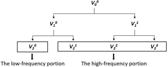
The real-time operation state of chemical factories can be assessed by analyzing the data of variables collected from industrial practice. However, disturbances may occur in different time-frequency ranges, which leads to the multi-scale features of the data. Appropriate multi-scale decomposition is not only assistant to eliminate random disturbances, but also conducive to local feature extraction, thus tend to improve the fault detection performance. Inspired by this, WPD is adopted in multi-scale decomposition of signals for its effectiveness in time-frequency analysis, and the schematic diagram of a two-layer wavelet packet decomposition example is given as in Figure 1.where $V_j^i$ represents the ith frequency band space of the jth scale. It can be seen from Figure 1 that the original signals are grouped into a high-frequency portion and a low-frequency portion with the adoption of WPD. Among them, only the wavelet coefficients in the lowest frequency band are assigned into the low-frequency portion, while the remaining coefficients are assigned into the high-frequency portion.

FIGURE 1

FIGURE 1. The schematic diagram of a two-layer wavelet packet decomposition.

Moreover, with the consideration of the online monitoring requirements in industrial practice, a moving window is introduced, in which the data in the moving window can be updated in real time for analysis, and the corresponding edge values are removed to prevent boundary effects.

Time-Frequency Analysis Based on Principal Component Analysis and Slow Feature Analysis

After the multi-scale decomposition introduced in Section 3.1, the high-frequency portion and the low-frequency portion of the original signals are obtained for the convenience of further feature extraction. As a matter of fact, only the low-frequency portion is reserved in many traditional time-frequency analysis algorithms. The neglect of the high-frequency portion will lead to the loss of important features, especially for pulse-type signals. Therefore, data information at all scales is retained in this research, and the classical PCA algorithm is applied to construct $T^2$ and SPE statistics in the high-frequency portion for further feature extraction. The long-term trend of the original signals is reflected in the low-frequency portion. With this concern, SFA is applied to construct $T^2, T_{e^2}, S^2 and S_e^2$ statistics in the low-frequency portion, which is assistant to the slowly changing feature extraction. It is noted that although the original signals are grouped into two portions, a multivariate statistical model is constructed for the wavelet coefficients at each scale. That is to say, taking the two-layer wavelet packet decomposition which is presented in Figure 1 as an example, one PCA model is constructed in the $V_0^2$ band space and three SFA models are constructed in the $V_2^1,V_2^2$ and $V_2^3$ band space, respectively.

Feature Fusion Based on Support Vector Data Description

After the time-frequency analysis introduced in Section 3.2, statistics which reflects the fundamental features of the original signals at different scales are obtained for the convenience of further fault detection. The statistics obtained under normal operating conditions are combined as the input of a SVDD model for training, and the radius of the hypersphere can be calculated as follows,

$R=\sqrt{\mathbf{1}-\mathbf{2}{\displaystyle \sum _{i=1}^n{\alpha }_{i}K\left(x_i,x_k\right)}-{\displaystyle \sum _{i=1}^n{\displaystyle \sum _{j=1}^n{\alpha }_i{\alpha }_{j}K\left(x_i,x_j\right)}}}(16)$

The Gaussian kernel function is introduced for its extensive applicability in this work. Then, the statistics obtained from the testing dataset are input into the trained SVDD model to calculated the distance between the testing sample points and the center of the hypersphere can be calculated as follows,

$D_{is}=\sqrt{\mathbf{1}-\mathbf{2}{\displaystyle \sum _{i=1}^n{\alpha }_{i}K\left(x_i,x_{test}\right)}-{\displaystyle \sum _{i=1}^n{\displaystyle \sum _{j=1}^n{\alpha }_i{\alpha }_{j}K\left(x_i,x_j\right)}}}(17)$

If $D_{is}\le R$, the sample point is considered as normal. Otherwise, the point will be indicated as an outlier.

Generally speaking, the most concerned issue in fault detection is the stability of the model and the alarm time of the fault. Inspired by this, two performance indicators of alarm latency (AL) and false alarm rate (FAR) are introduced for the model performance evaluation in this research, which are respectively given as,

$\text{AL}=\left({\text{S}}_A-{\text{S}}_I\right)\times SF(18)$

$\text{FAR}=\frac{FP}{FP+TN}(19)$

where the fault is introduced at the ${\text{S}}_A$-th sample point and detected at the ${\text{S}}_I$-th sample point, SF is the sampling frequency of the original data, FP are the number of normal samples that are indicated as anomalies incorrectly, FN is the number of fault samples without indication. 0 min alarm latency and 0% false alarm rate are expected to allow operators to provide an immediate treatment. Fault occurrence is determined at the end of three consecutive positive alarms, which is a common adopted rule to determine both the alarm time and false alarm rate, and the first consecutive positive alarm point is recorded.

The Framework of the Multi-Scale Process Monitoring Method Based on Time-Frequency Analysis and Feature Fusion

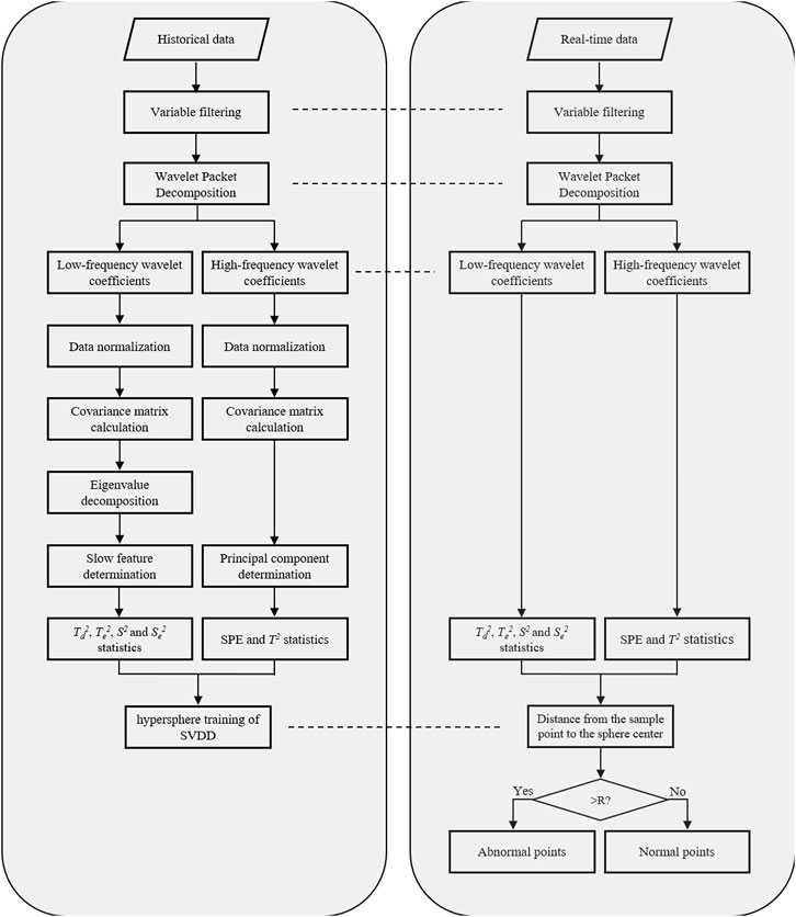
The complete method is conducted by off-line modeling and on-line monitoring, and the flowchart is represented in Figure 2. The corresponding procedures are described as follows.

FIGURE 2

FIGURE 2. The flow chart of the proposed multi-scale process monitoring method.

Off-Line Modeling

Step 1: Select historical data under normal operating conditions and monitoring variables.

Step 2: Decompose data into low-frequency portion and high-frequency portion.

Step 3: Normalize the obtained coefficients.

Step 4: Input the high-frequency coefficients into a PCA model to construct $T^2$ and SPE statistics.

Step 5: Input the low-frequency coefficients into an SFA model to construct $T^2, T_{e^2}, S^2 and S_{e^2}$ statistics.

Step 6: Input the model statistics at all scales into a SVDD model for training to determine the center and radius of the hypersphere.

On-Line Monitoring

Step 1: Obtain on-line detection values of monitoring variables.

Step 2: Decompose data into a low-frequency portion and a high-frequency portion with decomposition parameters from off-line modeling.

Step 3: Normalize the obtained on-line coefficients with corresponding parameters from off-line normalization.

Step 4: Input the high-frequency coefficients into the PCA model to obtain $T^2$ and SPE statistics.

Step 5: Input the low-frequency coefficients into the SFA model to obtain $T^2, T_{e^2}, S^2 and S_{e^2}$ statistics.

Step 6: Input the on-line statistics into the trained SVDD model for testing.

4 Case Study

In this section, the monitoring performance of the proposed multi-scale method is compared with the PCA and SFA algorithms at a single scale. Data obtained from the benchmark TEP and an industrial continuous catalytic reforming heat exchange unit are applied in this work to test the performance of the proposed method.

Case Study on Tennessee Eastman Process

4.1.1 Tennessee Eastman Process

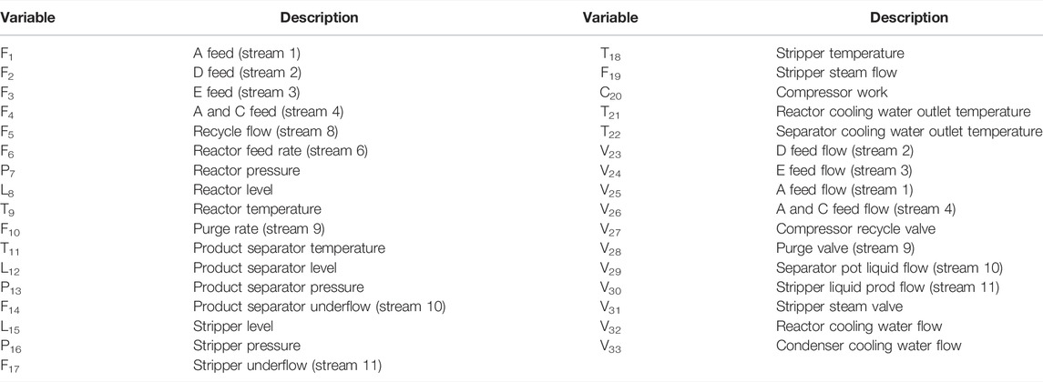
EP is a typical chemical process simulation benchmark developed by Eastman Chemical Company, and has been widely utilized to verify the performance of process monitoring algorithms. A reactor, a product condenser, a gas-liquid separator, a product desorption tower and a circulating compressor are contained in this process and the corresponding process flow chart is represented in Figure 3. There are 52 variables in TEP, including 22 continuous process variables, 19 synthetic variables and 11 manipulated variables. Considering the long sampling interval of the synthetic variables, the remaining 33 variables are finally selected in this paper, as shown in Table 1. A description of 21 preset faults is shown in Table 2, of which Fault 3, 9, 15, 21 are not taken into consideration in this work. The standard dataset consists of 500 training samples and 960 testing samples and the sampling frequency is 3 min. All faults in the testing dataset are introduced at the 160th sampling point.

FIGURE 3

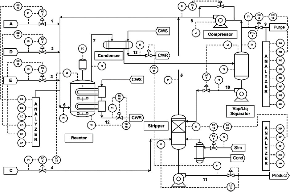
FIGURE 3. The flow chart of Tennessee Eastman Process (Bathelt et al., 2015).

TABLE 1

TABLE 1. Variables in Tennessee Eastman Process.

TABLE 2

TABLE 2. Faults in Tennessee Eastman Process.

4.1.2 Monitoring Results on Tennessee Eastman Process

In this section, the performance of the proposed method is verified on the benchmark TEP by comparing with PCA and SFA, which only focus on a single scale. In the PCA models at a single scale, the feature contribution parameter is 85%, and the thresholds of $T^2$ and SPE statistics are all determined at the 99% confidence level. In the SFA models at a single scale, $S_{e^2}$ the thresholds of $T^2, T_{e^2}, S^2 and S_{e^2}$ statistics are also all determined at the 99% confidence level, which is the same as the level in the PCA algorithm to ensure the fairness in the monitoring effect comparison. In the proposed models, the width of the on-line moving window is 60 and the corresponding moving step is 1. The classic $db4$ wavelet basis function is adopted to a two-layer wavelet packet decomposition. After the decomposition, the feature contribution parameter used in the PCA models is also 85%. Then, the statistics constructed by PCA and SFA are processed by SVDD for process monitoring. The parameters of the penalty coefficients and variances of the Gaussian kernel function are optimized according to the alarm latency results.

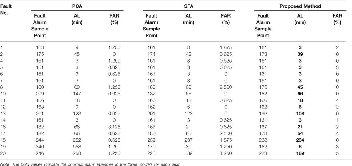
In this research, two performance indicators of alarm latency and false alarm rate are introduced for model performance evaluation. 0 min alarm latency and 0% false alarm rate are expected to allow operators to provide an immediate treatment. Disturbances are all introduced at the 160th sample, and the detailed monitoring results are given in Table 3. Models that raise fault alarms frequently would result in misleading conclusions, thus making them untrustworthy. It can be seen from Table 3 that the false alarm rates of these faults are all no higher than 5%, which indicates that the fault detection effect of the models is stable, and then the performance of these models can be compared by alarm latencies.

TABLE 3

TABLE 3. Fault alarm results of PCA, SFA and the proposed method in the TEP dataset.

As shown in Table 3, SFA has a generally better monitoring performance than PCA for its earlier fault detection. The core idea of SFA is to extract the slowly changing components from the time-variant data series as the fundamental features. Moreover, among the performance of these three methods, the alarm latencies of these three methods are the same in most step faults, specifically including Faults 4,5,6,7. That’s because the features of pulse-type signal are extracted in the step fault detection, which are contained in the high-frequency portion. SFA is beneficial to the slowly changing feature extraction, but it has no advantage over PCA in high-frequency feature extraction. The PCA algorithm is also adopted for the high-frequency feature extraction in the proposed method, consequently leading to the same performance when compared with the PCA and SFA. On the whole, the proposed multi-scale method performs best among these three methods. Although the alarm latencies of these three methods are the same in some faults, faults can be identified first by the proposed multi-scale method in the others. The classical PCA algorithm is applied in the high-frequency portion containing the pulse and noise. And due to the good performance on dynamic feature extraction of SFA, it is selected in the low-frequency portion that reflects the long-term trend of signals. Features at different scales are extracted by the novel proposed multi-scale method, thus the immediate alarm of faults is realized.

The monitoring results of Faults 5 and 13 in the standard TEP dataset are represented in Figure 4 and Figure 5 respectively. It is noted that the process monitoring graphs of PCA are based on SPE statistics due to the slower alarming of $T^2$. Fault 5 is generated with a step change in the condenser cooling water inlet temperature. Using these three methods, Fault 5 can be identified with a low false alarm rate of 3% in 3 min, because of the same processing capability as the pulse-type signal. Fault 13 is generated with a slow drift change in the reaction kinetics. The false alarm rates of Fault 13 in these three methods are 1%. Compared with PCA and SFA, the fault can be identified 15 min earlier in the proposed multi-scale method. That can be interpreted as that the autocorrelation of sequences is approximately weakened by WPD, and then several statistics are constructed at each scale for the local feature extraction after multi-scale decomposition, which demonstrates that the multi-scale feature extraction can be better captured by the proposed method.

FIGURE 4

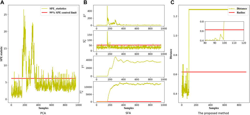
FIGURE 4. The Fault monitoring graphs of Fault 5 in the TEP dataset corresponding to three different models: (A) PCA model, (B) SFA model and (C) The proposed multi-scale model.

FIGURE 5

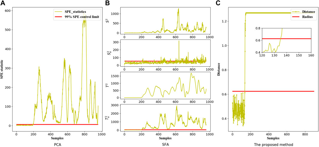
FIGURE 5. The Fault monitoring graphs of Fault 13 in the TEP dataset corresponding to three different models: (A) PCA model, (B) SFA model and (C) The proposed multi-scale model.

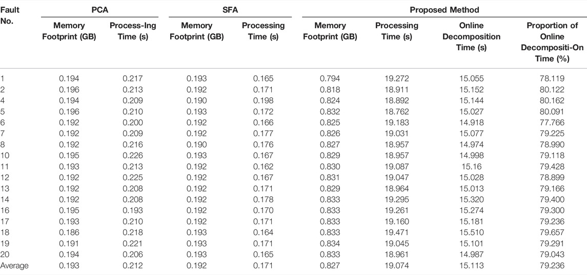
Although with the application of the proposed method, these faults can be detected earlier than the other two algorithms, it is noted that a higher computational load is consumed for its more complicated procedures. The proposed method is evaluated using Intel core TM i5-3470 CPU with 3.20 GHz, and the detailed computation load results of the TEP dataset, containing the memory footprint and processing time, are given in Table 4. It can be seen from Table 4 that, compared with the PCA and SFA algorithms at a single scale, a higher memory footprint and longer processing time are consumed in this novel method, within which more than 75% of the time is consumed on online multi-scale decomposition. On this basis, how to reduce the computational load of this proposed method to make it more suitable for online process monitoring is the focus of future work. In the TEP dataset, the sampling frequency is 3 min, while the average time consumed in online processing of a single test dataset is 12.094 s, because of which it can be deduced that the online processing time of a single sampling point is less than the sampling frequency of the TEP dataset. In conclusion, it is feasible to apply the proposed algorithm to this dataset in terms of the computational load.

TABLE 4

TABLE 4. The computational load of PCA, SFA and the proposed method in the TEP dataset.

4.2 Case Study on an Industrial Continuous Catalytic Reforming Process

4.2.1 Industrial Continuous Catalytic Reforming Process

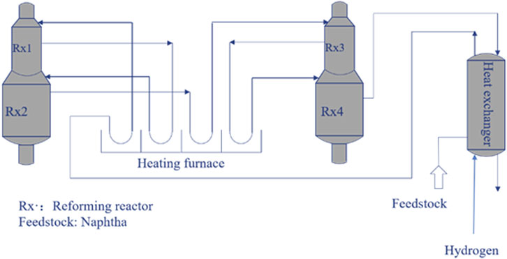
The proposed multi-scale process monitoring method, based on time-frequency analysis and feature fusion, is applied to an industrial continuous reforming process. Four reactors, four furnaces and a plate exchanger are contained in this process and the corresponding process flow chart is represented in Figure 6. The sampling frequency is 1 min. There are 27 variables finally selected in this paper, as shown in Table 5. The pressure drop of the plate exchanger is an important monitoring variable, which is affected by various factors such as production load and ambient temperature. The increase in pressure drop is difficult to detect in time due to its slow changing rate. It is necessary to establish a monitoring model for this process.

FIGURE 6

FIGURE 6. The flow chart of the industrial continuous catalytic reforming heat exchange unit.

TABLE 5

TABLE 5. Process variables in the industrial continuous catalytic reforming unit.

4.2.2 Monitoring Results on the Industrial Continuous Catalytic Reforming Process

In this section, the performance of the proposed method is verified on a slow changing pressure drop of the plate exchanger by comparing with PCA and SFA. In the PCA and SFA models which only focus on a single scale, the feature contribution parameter is 85%, and the thresholds of all statistics are all determined at the 99% confidence level to provide a fair comparison of fault detection effects. In the proposed models, the width of the on-line moving window is 60 and the corresponding moving step is 1. The classic $db4$ wavelet basis function is adopted to a two-layer wavelet packet decomposition. After the decomposition, the applied feature contribution parameter is also 85%. Then, the statistics constructed by PCA and SFA are combined and processed by SVDD for fault detection. The parameters of the penalty coefficients and variances of the Gaussian kernel function are optimized according to the alarm latency results.

The detailed monitoring results of these three methods are presented in Figure 7, which reveals that all these three data-driven algorithms have achieved to detect the pressure drop fault on the industrial continuous catalytic reforming unit. The FARs, based on PCA, SFA and the proposed method, are 6.175, 5.873 and 0.338%, respectively, which indicates that the stability of these three methods applied to the industrial data is acceptable, thus demonstrating that the corresponding fault detection results are reliable. The faults are identified at the 665th, 665th, and 652nd sampling points, which indicates that the proposed multi-scale method exhibits the best monitoring performance and the fault can be identified 13 min earlier than the other two methods at a single scale, thus demonstrating the existence of multi-scale features in an industrial process. That’s because the original signal is decomposed into a low-frequency portion and a high-frequency portion, and features are extracted separately with this proposed method. Not only the interpretability of the model is improved, but also more effective slowly changing information is extracted with this multi-scale monitoring method.

FIGURE 7

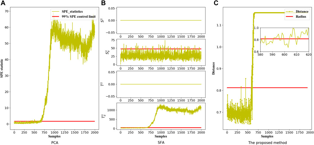
FIGURE 7. The fault monitoring graphs of the industrial continuous catalytic reforming heat exchange unit corresponding to three different models: (A) PCA model, (B) SFA model and (C) The proposed multi-scale model.

5 Conclusion

In this paper, a multi-scale process monitoring method based on time-frequency analysis and feature fusion is proposed. Considering that process disturbances may occur in arbitrary time and frequency, wavelet packet decomposition is utilized for multi-scale data decomposition. Then the classical PCA algorithm is applied for the high-frequency portion, and the SFA algorithm is applied for the low-frequency portion to extract the slowly changing features of the original signals. With the application of the SVDD algorithm, statistics at different scales are fused to provide an overall fault detection result. Case studies on the TEP and an industrial continuous catalytic reforming heat exchange unit show the superiority of the proposed method compared with the corresponding multivariate statistical feature extraction algorithms, which only focus on a single scale. The proposed method provides a multi-scale perspective for solving practical industrial process monitoring problems. However, more research on the computational load optimization and the effect of different levels of noise needs to be carried out in future.

Data Availability Statement

The data that support the findings of this study are available from BUCTPSE but restrictions apply to the availability of these data, which were used under license for the current study, and so are not publicly available. Data are however available from the authors upon reasonable request and with permission of BUCTPSE.

Author Contributions

CJ: Conceptualization, Methodology, Writing, original draft preparation, Writing—review and editing, Visualization; TT: Conceptualization, Investigation, Writing—review and editing; JW: Conceptualization, Resources, Supervision, Project administration; WS: Conceptualization, Methodology, Resources, Supervision, Project administration.

Conflict of Interest

The authors declare that the research was conducted in the absence of any commercial or financial relationships that could be construed as a potential conflict of interest.

Publisher’s Note

All claims expressed in this article are solely those of the authors and do not necessarily represent those of their affiliated organizations, or those of the publisher, the editors and the reviewers. Any product that may be evaluated in this article, or claim that may be made by its manufacturer, is not guaranteed or endorsed by the publisher.

References

Bathelt, A., Ricker, N. L., and Jelali, M. (2015). Revision of the Tennessee Eastman Process Model. IFAC-PapersOnLine 48 (8), 309–314. doi:10.1016/j.ifacol.2015.08.199

CrossRef Full Text | Google Scholar

Bentley, P. M., and McDonnell, J. T. E. (1994). Wavelet Transforms: an Introduction. Electron. Commun. Eng. J. 6 (4), 175–186. doi:10.1049/ecej:19940401

CrossRef Full Text | Google Scholar

Burrus, C. S., Gopinath, R. A., and Guo, H. (1998). Introduction to Wavelets and Wavelet Transforms: A Primer. New Jersey: Prentice-Hall.

Google Scholar

Choqueuse, V., Benbouzid, M. E. H., Amirat, Y., and Turri, S. (2012). Diagnosis of Three-phase Electrical Machines Using Multidimensional Demodulation Techniques. IEEE Trans. Ind. Electron. 59 (4), 2014–2023. doi:10.1109/tie.2011.2160138

CrossRef Full Text | Google Scholar

Comon, P. (1994). Independent Component Analysis, a New Concept? Signal Process. 36 (3), 287–314. doi:10.1016/0165-1684(94)90029-9

CrossRef Full Text | Google Scholar

Deng, Z., Han, T., Cheng, Z., Jiang, J., and Duan, F. (2022). Fault Detection of Petrochemical Process Based on Space-Time Compressed Matrix and Naive Bayes. Process Saf. Environ. Prot. 160, 327–340. doi:10.1016/j.psep.2022.01.048

CrossRef Full Text | Google Scholar

Geladi, P., and Kowalski, B. R. (1986). Partial Least-Squares Regression: a Tutorial. Anal. Chim. Acta 185, 1–17. doi:10.1016/0003-2670(86)80028-9

CrossRef Full Text | Google Scholar

Ghobakhloo, M. (2020). Industry 4.0, Digitization, and Opportunities for Sustainability. J. Clean. Prod. 252, 119869. doi:10.1016/j.jclepro.2019.119869

CrossRef Full Text | Google Scholar

Ha Quang Minh, H. Q., and Wiskott, L. (2013). Multivariate Slow Feature Analysis and Decorrelation Filtering for Blind Source Separation. IEEE Trans. Image Process. 22 (7), 2737–2750. doi:10.1109/tip.2013.2257808

PubMed Abstract | CrossRef Full Text | Google Scholar

Hardoon, D. R., Szedmak, S., and Shawe-Taylor, J. (2004). Canonical Correlation Analysis: An Overview with Application to Learning Methods. Neural Comput. 16 (12), 2639–2664. doi:10.1162/0899766042321814

PubMed Abstract | CrossRef Full Text | Google Scholar

Huang, J., Ersoy, O. K., and Yan, X. (2017). Slow Feature Analysis Based on Online Feature Reordering and Feature Selection for Dynamic Chemical Process Monitoring. Chemom. Intelligent Laboratory Syst. 169, 1–11. doi:10.1016/j.chemolab.2017.07.013

CrossRef Full Text | Google Scholar

Jutten, C., and Karhunen, J. (2004). Advances in Blind Source Separation (BSS) and Independent Component Analysis (ICA) for Nonlinear Mixtures. Int. J. Neur. Syst. 14 (05), 267–292. doi:10.1142/s012906570400208x

PubMed Abstract | CrossRef Full Text | Google Scholar

Misra, M., Yue, H. H., Qin, S. J., and Ling, C. (2002). Multivariate Process Monitoring and Fault Diagnosis by Multi-Scale PCA. Comput. Chem. Eng. 26 (9), 1281–1293. doi:10.1016/S0098-1354(02)00093-5

CrossRef Full Text | Google Scholar

Nawaz, M., Maulud, A. S., Zabiri, H., Taqvi, S. A. A., and Idris, A. (2021). Improved Process Monitoring Using the CUSUM and EWMA-Based Multiscale PCA Fault Detection Framework. Chin. J. Chem. Eng. 29, 253–265. doi:10.1016/j.cjche.2020.08.035

CrossRef Full Text | Google Scholar

Portnoff, M. (1980). Time-frequency Representation of Digital Signals and Systems Based on Short-Time Fourier Analysis. IEEE Trans. Acoust. Speech, Signal Process. 28 (1), 55–69. doi:10.1109/tassp.1980.1163359

CrossRef Full Text | Google Scholar

Qin, S. J. (2012). Survey on Data-Driven Industrial Process Monitoring and Diagnosis. Annu. Rev. Control 36 (2), 220–234. doi:10.1016/j.arcontrol.2012.09.004

CrossRef Full Text | Google Scholar

Severson, K., Chaiwatanodom, P., and Braatz, R. D. (2016). Perspectives on Process Monitoring of Industrial Systems. Annu. Rev. Control 42, 190–200. doi:10.1016/j.arcontrol.2016.09.001

CrossRef Full Text | Google Scholar

Shang, C., Yang, F., Gao, X., Huang, X., Suykens, J. A. K., and Huang, D. (2015). Concurrent Monitoring of Operating Condition Deviations and Process Dynamics Anomalies with Slow Feature Analysis. AIChE J. 61 (11), 3666–3682. doi:10.1002/aic.14888

CrossRef Full Text | Google Scholar

Sprekeler, H., Zito, T., and Wiskott, L. (2014). An Extension of Slow Feature Analysis for Nonlinear Blind Source Separation. J. Mach. Learn. Res. 15 (1), 921–947.

Google Scholar

Tax, D. M. J., and Duin, R. P. W. (2004). Support Vector Data Description. Mach. Learn. 54 (1), 45–66. doi:10.1023/b:mach.0000008084.60811.49

CrossRef Full Text | Google Scholar

Wold, S., Esbensen, K., and Geladi, P. (1987). Principal Component Analysis. Chemom. Intelligent Laboratory Syst. 2 (1-3), 37–52. doi:10.1016/0169-7439(87)80084-9

CrossRef Full Text | Google Scholar

Xiu, X., Yang, Y., Kong, L., and Liu, W. (2021). Data-driven Process Monitoring Using Structured Joint Sparse Canonical Correlation Analysis. IEEE Trans. Circuits Syst. II 68 (1), 361–365. doi:10.1109/tcsii.2020.2988054

CrossRef Full Text | Google Scholar

Xiu, X., Yang, Y., Kong, L., and Liu, W. (2020). Laplacian Regularized Robust Principal Component Analysis for Process Monitoring. J. Process Control 92, 212–219. doi:10.1016/j.jprocont.2020.06.011

CrossRef Full Text | Google Scholar

Yin, S., Ding, S. X., Xie, X., and Luo, H. (2014). A Review on Basic Data-Driven Approaches for Industrial Process Monitoring. IEEE Trans. Ind. Electron. 61 (11), 6418–6428. doi:10.1109/tie.2014.2301773

CrossRef Full Text | Google Scholar

Zhang, Y., and Ma, C. (2011). Fault Diagnosis of Nonlinear Processes Using Multiscale KPCA and Multiscale KPLS. Chem. Eng. Sci. 66 (1), 64–72. doi:10.1016/j.ces.2010.10.008

CrossRef Full Text | Google Scholar

Zhang Zhang, Z., and Dacheng Tao, D. (2012). Slow Feature Analysis for Human Action Recognition. IEEE Trans. Pattern Anal. Mach. Intell. 34 (3), 436–450. doi:10.1109/tpami.2011.157

PubMed Abstract | CrossRef Full Text | Google Scholar

Zhongming Ye, Z., Bin Wu, B., and Sadeghian, A. (2003). Current Signature Analysis of Induction Motor Mechanical Faults by Wavelet Packet Decomposition. IEEE Trans. Ind. Electron. 50 (6), 1217–1228. doi:10.1109/tie.2003.819682

CrossRef Full Text | Google Scholar

Žvokelj, M., Zupan, S., and Prebil, I. (2010). Multivariate and Multiscale Monitoring of Large-Size Low-Speed Bearings Using Ensemble Empirical Mode Decomposition Method Combined with Principal Component Analysis. Mech. Syst. Signal Process. 24 (4), 1049–1067. doi:10.1016/j.ymssp.2009.09.002

CrossRef Full Text | Google Scholar