Frequency-independent damping models for a high-rise building with simultaneous horizontal and vertical seismic motions

Recent seismic analyses indicate that the structural damping ratio should be considered frequency-independent, for safe and accurate estimations. In response, damping models like the Wilson–Penzien (WP) damping model, that is one of the modal damping, provide frequency independence across all modes; however, these models require considerable computational resources, especially for large-scale models. While Rayleigh damping is computationally efficient, it maintains a nearly constant damping ratio only within a limited frequency range. To address these limitations, several alternative damping models have been introduced, such as uniform (UN), causal hysteretic (CH), and extended Rayleigh (ER). We use the factor W_ξ to represent the frequency range where the damping ratio remains approximately constant, defined as the ratio of maximum to minimum frequencies (f_max/f_min), within a specified tolerance of the target damping ratio. For Rayleigh damping, W_ξ = 3.7, while the CH and ER models achieve W_ξ values greater than 20. Although the UN model achieves a high W_ξ, it demands large computational resources in the implicit analyses, commonly used for seismic response studies. In this study, we address the simultaneously inputting horizontal and vertical seismic motion into a large-scale dynamic analysis model of a high-rise building. In this analysis, horizontal, vertical, and local beam vibration modes spanning a wide frequency range appeared. Considering that these modes require the same damping ratio, damping models with W_ξ values of 50 or higher are desirable. However, this threshold considerably exceeds W_ξ values achievable with the existing models, rendering these models unsuitable for the intended application. Therefore, we propose and validate the efficiency of two new damping models (ER-W and CH19) that meet this requirement by improving existing models. Using these damping models, it is possible to analyze the horizontal and vertical modes and local vibration modes of the beam, assuming a simultaneous horizontal and vertical input to a high-rise building.

1 Introduction

Damping in buildings substantially impacts seismic response assessments. It can be broadly classified into two categories: inherent damping that occurs within the linear range, and plastic damping that arises from material plasticization. This study focuses on the inherent damping. Although the damping ratio (ξ) of a building’s first-order mode is generally well-known, the ξ values for higher-order modes remain less understood. However, recent evidence suggests these values are similar to or slightly exceed those of the primary mode (Nakamura et al., 2017). As a conservative measure for seismic design, it is assumed that the ξ for higher-order modes should match the first-order mode’s damping ratio. Consequently, for all modes considered in the response analysis, ξ is treated as constant and independent of the vibration frequency. Three prevalent damping models in seismic response analyses are stiffness-proportional, Rayleigh, and modal damping (Figure 1). In stiffness-proportional damping, the ξ set for primary modes is amplified for higher-order modes, while modal damping allows for the customization of ξ across all modes. However, as the number of analytical degrees of freedom (DOFs) increases, so does the computational load, making modal damping less feasible for large-scale models.

Figure 1

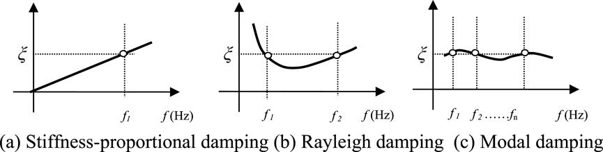
Figure 1. Representative damping model available for time history analysis. (A) Stiffness-proportional damping (B) Rayleigh damping (C) Modal damping.

Rayleigh damping combines mass- and stiffness-proportional damping (Figure 2), allowing the assignment of target damping ratios (ξ_aim) at two specific frequencies. Between these frequencies, ξ remains relatively close to ξ_aim, and the computational load is manageable, making Rayleigh damping a widely used choice in many analyses. However, its adaptive-frequency range where ξ is almost constant is narrow, limiting its accuracy in capturing responses across low- and high-order modes, presenting a notable challenge with Rayleigh damping. In addition, issues with Rayleigh damping have been discussed by Hall (2006).

Figure 2

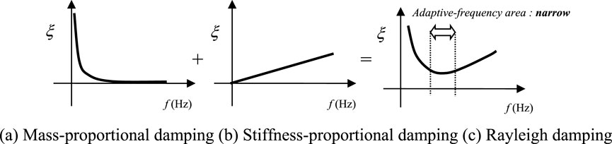
Figure 2. Rayleigh damping. (A) Mass-proportional damping (B) Stiffness-proportional damping (C) Rayleigh damping.

With recent advancements in computational power and analytical methods, several studies have investigated seismic responses using large-scale FE models of structures, i.e., (Ichihara et al., 2021). In addition, more analyses now incorporate both horizontal and vertical seismic wave components. Typically, vertical modes exhibit higher frequencies than their horizontal counterparts. According to Kinoshita et al. (2021), if the primary horizontal vibrational frequency of a skyscraper is 0.2 Hz, its primary vertical frequency reaches 2.6 Hz, which is 13 times higher. Mogi et al. (2023) conducted a study on a high-rise building using a large-scale model, demonstrating that in addition to primary modes, local beams resonate within the 5.0–7.2 Hz range. In this study, this analysis model is used as an example model. To ensure frequency independence of damping across all modes for more complex building models, we set a target W_ξ of 50 supposing f_min = 0.2 Hz and f_max = 10 Hz.

The following assumptions are made in the analysis of this paper as a conservative assumption, and all of the damping models examined in this paper correspond to these assumptions. If these assumptions change, the appropriate damping model will also differ.

1) The damping ratios of the higher-order horizontal modes are the same as the damping ratio of the first horizontal vibration mode.

2) The damping ratios of the vertical modes and local modes are also the same as the damping ratio of the first horizontal vibration mode.

Earlier, Nakamura (2007) introduced the causal hysteretic (CH) damping model, achieving frequency independence by restricting the frequency range under consideration. This model represents a time–domain approximation of complex damping, 1 + 2ξi, derived from the frequency domain, where i indicates an imaginary unit. Extended Rayleigh (ER) damping model was developed by integrating the CH model, instead of the stiffness-proportional damping model (Figure 3) and was subsequently validated by Nakamura (2016). These models further demonstrated their effectiveness in addressing nonlinear analyses (Nakamura et al., 2023).

Figure 3

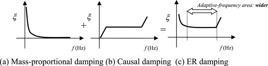
Figure 3. Extended Rayleigh (ER) damping. (A) Mass-proportional damping (B) Causal damping (C) ER damping.

Hereafter, W_ξ denotes the extent of the adaptive-frequency range, defined as the ratio of the maximum frequency f_max to minimum frequency f_min that remains within a specific tolerance relative to the target damping ratio. This concept aligns with Hall (2006), who demonstrated that for Rayleigh damping, the frequency range spans from $\widehat{\omega }$ to R $\widehat{\omega }$ when the obtained damping ratio is within the range of ξ_min = ξ-Δ and ξ_max = ξ + Δ, for the desired damping ratio ξ. In this paper, we express the desired damping ratio ξ as ξ_aim, Δ/ξ as “the allowable tolerance,” and amount of the adaptive-frequency area R as W_ξ. For instance, at a tolerance range of ±10%, W_ξ is 3.7 for Rayleigh damping, whereas for CH and ER models, it exceeds 20. However, this study aims to achieve a W_ξ above 50 and proposes two models (ER-W and CH19).

Uniform damping (UN) introduced by Huang et al. (2019) manifests an impressively extensive frequency-independent range. However, it requires very fine time–step intervals, making it suitable for explicit analyses, but increasing the computational load in implicit analyses due to these finely spaced intervals. In addition, this model poses challenges related to the frequency-dependent behavior of dynamic stiffness, as highlighted by Mogi et al. (2023). These damping models are outlined and compared in this paper.

2 Classical damping models

Certain classical and commonly used models in various analyses are discussed below.

2.1 Wilson–Penzien model (WP)

Wilson–Penzien model (WP), developed by Wilson and Penzien (1972), is a type of modal damping model that provides a constant damping ratio across all frequencies. Damping matrix in this model is based on initial elastic eigenvalues and remains unchanged, even as the structure enters the nonlinear domain. Chopra and McKenna (2016) demonstrated that response variations are minimal, even without updating the damping matrix as the structure evolves. However, a limitation of this model lies in its requirement for extensive eigenvalue analyses across very many modes. Given that the damping matrix is a full matrix, the computational load becomes notable for large-scale models, often hindering its application.

2.2 Rayleigh model

Considering [M], [K], and {u (t)} as the mass matrix, stiffness matrix, and displacement vector of the structure, respectively, the equation of motion can be expressed as Equation 1, where {D (t)} represents the damping force vector.

$\left[M\right]\left\{\ddot{u}\left(t\right)\right\}+\left\{D\left(t\right)\right\}+\left[K\right]\left\{u\left(t\right)\right\}=\left\{0\right\}(1)$

In Equation 1, the Rayleigh damping model is represented by Equation 2.

$\left\{D\left(t\right)\right\}=\left(\alpha \left[M\right]+\beta \left[K\right]\right)\left\{\dot{u}\left(t\right)\right\}(2)$

Coefficients α and β are determined based on two circular frequencies, ω₁ and ω₂ (or the two frequencies f₁ and f₂), along with the target damping ratio ξ_aim, as shown in Equation 3. The accuracy R_ξ(f) of the damping ratio ξ according to f with respect to ξ_aim is expressed by Equation 4. When f < f₁ or f₂ < f, R_ξ(f) > 1, for f₁ < f < f₂, then R_ξ(f) < 1.

$\alpha =\frac{2{\xi }_{aim}{\omega }_1{\omega }_2}{{\omega }_1+{\omega }_2}=\frac{4\pi {\xi }_{aim}{f}_1{f}_2}{f_1+f_2},\hspace{1em}\beta =\frac{2{\xi }_{aim}}{{\omega }_1+{\omega }_2}=\frac{{\xi }_{aim}}{\pi \left(f_1+f_2\right)}(3)$

$R_{\xi }\left(f\right)=\frac{\xi \left(f\right)}{{\xi }_{aim}},\hspace{1em}\xi \left(f\right)=\frac{1}{2}\left(\frac{\alpha }{\omega }+\beta \omega \right)=\frac{\alpha }{4\pi f}+\pi f\beta (4)$

This study aims to maintain a consistent damping ratio, ξ_aim, over an extensive frequency range during time–history response analysis. However, Rayleigh damping achieves this only within a narrow range around the two specified frequencies, f₁ and f₂. Consequently, this research seeks to expand Rayleigh damping’s adaptive-frequency range by defining an allowable area in the damping ratio, termed as the tolerance level. For Rayleigh damping, the W_ξ values are 2.5, 3.7, and 6.9 when tolerances are set at 5%, 10%, and 20% of ξ_aim, respectively. Figure 4 depicts W_ξ with a 10% tolerance, whereas Table 1 enumerates W_ξ values for various tolerance thresholds in Rayleigh damping. In this damping model, there is an option to use [K] in Equation 2 as either the initial stiffness or the tangent stiffness (Jehel et al., 2014).The former approach is referred to as the initial Rayleigh model, and the latter as the tangent Rayleigh model. If the tangent [K] is used, eigen frequencies f₁ and f₂ must be modified, but it is common practice to keep these frequencies fixed and replace only [K] with the tangent stiffness.

Figure 4

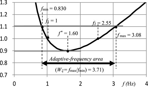
Figure 4. W_ξ(f) of Rayleigh damping (tolerance 10% and f₁ = 1).

Table 1

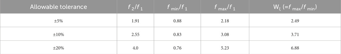
Table 1. Allowable tolerance of the damping ratio and adaptive-frequency range for Rayleigh damping.

3 Recently proposed model

Several models have been proposed in recent years to achieve frequency-independent damping for nonlinear time–domain analyses. For example, capped viscous damping (Hall, 2006; Mogi et al., 2022), an inherent damping model using virtual viscous dampers with uniform damping constants (Kitayama and Constantinou, 2022), rate-independent linear damping incorporated into a base-isolated structure (Wu et al., 2023), UN (Huang et al., 2019), bell-shaped damping (Lee, 2021), CH (Nakamura, 2007), and ER (Nakamura, 2016) models. This section provides an overview of the UN, CH, and ER models, which are regarded as highly suitable for general seismic analyses.

3.1 Uniform damping model (UN)

Huang et al. (2019) and Tian et al. (2022) introduced a novel damping model based on frequency-independent damping theory that ensures consistent damping across a wide frequency range. Integrated into FE programs, such as LS-DYNA (Livermore Software Technology Corporation, 2021), this model is used in impact analysis. Recently, this model is also installed in OPENSEES (Tian et al., 2023). Generally, the damping ratio remains almost constant across a broad frequency scope. To streamline calculations, a differential approximation is used to evaluate the filtering process, implying a potential decrease in accuracy of the damping ratio if the time increment, Δt, is extended. Although this damping model is predominantly used for explicit methods, where refining Δt poses minimal issues, caution is advised when employing it for implicit methods. This model amplifies dynamic stiffness, altering natural frequencies of the building. No effective countermeasure exists for this phenomenon; therefore, the user manual advises direct correction of building stiffness by adjusting the Young’s modulus (Mogi et al., 2023). Hereafter, the original UN model is abbreviated as UN0, and the stiffness-modified model as UN1. Lee (2021) proposed bell-shaped proportional viscous damping models for the same purpose.

3.2 Causal hysteretic damping (CH)

Nakamura (2007) introduced the CH model, a damping approach that achieves frequency independence by limiting the considering frequency range. This model represents a time–domain transformation of complex damping (1 + 2ξi, where i is an imaginary unit) from the frequency domain. Since i does not adhere to the causality law and is thus not convertible to the time–domain (Inaudi and Kelly, 1995), an approximate imaginary unit (Figure 5) that complies with causality, is employed to develop a suitable damping model for time–history response analysis. By transforming this an approximate imaginary unit to the time–domain, the impulse response function can be obtained. This function can be effectively applied to the time–history analyses.

Figure 5

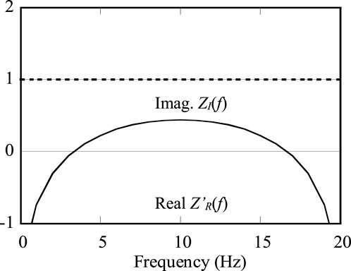
Figure 5. Approximate imaginary unit function (Z′) (f).

Equation 5 defines the damping force vector {D(t)} for the CH model, where [K] denotes the stiffness matrix, $\left\{\dot{u}\left(t\right)\right\}$ indicates the velocity vector at the current time t, and {u (t - j × Δt)} is a displacement vector prior to time t by j × Δt. This equation modifies the stiffness-proportional damping, proportional to the current velocity in the first term, by the coefficient sum of past displacements in the second term (Figure 6). The damping force vector {D(f)} in the frequency domain is expressed by Equation 6. For nonlinear analysis, there is a choice of [K] as either the initial stiffness or the tangential stiffness at each time step. In this paper, the tangential stiffness is used in all cases.

$\left\{D\left(t\right)\right\}=2\xi \left[K\right]\cdot \left(a_0\cdot \left\{\dot{u}\left(t\right)\right\}+{\displaystyle \sum _{j=1}^N}{b}_j\left\{u\left(t-j\cdot \Delta t\right)\right\}\right)(5)$

$\left\{D\left(f\right)\right\}=2\xi \left(2\pi f\cdot i\cdot a_0+{\displaystyle \sum _{j=1}^N}{b}_j\cdot e^{-2\pi f\cdot i\cdot j\Delta t}\right)\cdot \left[K\right]\left\{u\left(f\right)\right\}(6)$

Figure 6

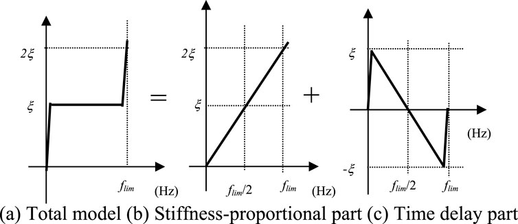
Figure 6. Causal damping model. (A) Total model (B) Stiffness-proportional part (C) Time delay part.

N corresponds to the number of past displacements considered. Depending on N, several models can be constructed. We used two-term, four-term, and nine-term models. Increasing the number of terms enhances both the W_ξ value and model accuracy, but also increases computational demand. The values of a₀ and b_j for each model are listed in Table 2. The highest W_ξ is obtained in the nine-term model (hereafter, CH9). Figure 7A shows R_ξ(f) for CH9 when ξ_aim is 0.01, 0.03, and 0.05 and f_lim is 10 Hz. The differences in R_ξ(f) across each ξ_aim are minimal. A peak appears in the low-frequency range approximately 0.8 Hz, and the tolerance was based on this peak value. Figure 7A shows that the tolerance is 11% and W_ξ is 25.8 for ξ_aim = 0.03.

Table 2

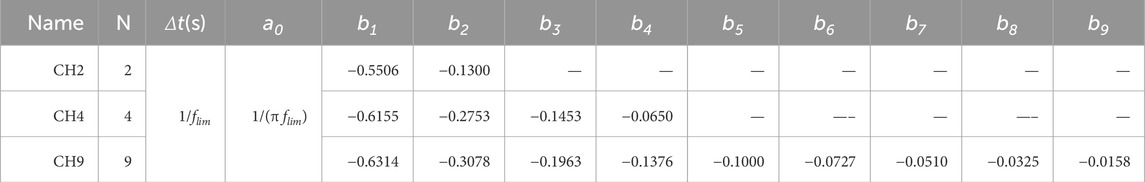
Table 2. Coefficients of CH2, CH4, and CH9.

Figure 7

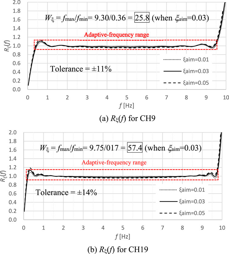
Figure 7. Comparison of W_ξ of the CH model. (A) R_ξ(F) for CH9 (B) R_ξ(F) for CH19.

3.3 Extended Rayleigh damping (ER)

Although Rayleigh damping is a straightforward and useful technique, it is primarily limited by its narrow adaptive-frequency range. While Rayleigh damping combines mass-proportional and stiffness-proportional components, in the ER model, the stiffness-proportional damping is replaced by the two-term CH model (Figure 3).

Within the ER framework, two models were developed to minimize the allowable tolerance for the target damping ratio ξ_aim, within the adaptive-frequency range. The range for ξ_aim. is set between 0.01 and 0.10. These models accommodate allowable tolerances of ±5% and ±10% and are termed high- and medium-accuracy models, respectively, as described by (Nakamura, 2016). Hereinafter, the high-accuracy model is referred to as ER-H, and the medium-accuracy model as ER-M.

The damping force vector, {D(t)}, is expressed in Equation 7, where a₀, b₁, and b₂ represent the coefficients of the two-term CH model. Coefficients C₀ to C₂ are adjusted based on ξ_aim (Table 3). Equation 8 presents the theoretical expression for ξ(f), whereas the accuracy R_ξ(f) with respect to ξ_aim is shown in Equation 9, where f_lim denotes the upper frequency limit set by the CH model. Figure 8A and (b) display R_ξ(f) values for ER-H and ER-M when ξ_aim is 0.01, 0.03, or 0.05, with an f_lim of 10 Hz. As observed in these figures, R_ξ is large below 0.7 Hz, decreases below 1 between 0.7 and 1.2 Hz, exceeds 1 between 1.2 and 4 Hz, remains close to 1 between 4 and 8 Hz, and finally increases beyond 8 Hz. This pattern aligns with the characteristics shown in Figure 3C. When ξ_aim is 0.03, the W_ξ is 13.7 for ER-H in Figure 8A and 21.5 for ER-M in Figure 8B. The applicability of these models to nonlinear analyses has also been confirmed (Ota et al., 2023).

$\left.\begin{array}{l}\left\{D\left(t\right)\right\}=\left({{\alpha }_0}^{\prime }\left[M\right]+{{\alpha }_1}^{\prime }\left[K\right]\right)\left\{\dot{u}\left(t\right)\right\}+2{\xi }_{aim}\left[K\right]\cdot \left({\gamma }_1^{\prime }\left\{u\left(t-{t_{\mathrm{l}}}_{\text{im}}\right)\right\}+{\gamma }_2^{\prime }\left\{u\left(t-2{t_{\mathrm{l}}}_{\text{im}}\right)\right\}\right)\\ a_0=\frac{1}{\left(\pi \cdot f_{\lim }\right)},b_1=-0.551,b_2=-0.130,t_{\lim }=\frac{1}{f_{\lim }\left(s\right)}\\ {{\alpha }_0}^{\prime }=2{\xi }_{aim}{f}_{\lim }{C}_0,{{\alpha }_1}^{\prime }=2{\xi }_{aim}{a}_0\left(C_1+C_2\right),{\gamma }_1^{\prime }=2{\xi }_{aim}{C}_1{b}_1,{\gamma }_2^{\prime }=2{\xi }_{aim}{C}_1{b}_2,\end{array}\right\}(7)$

$\left.\begin{array}{l}{\xi }^{\prime }\left(f\right)\approx \frac{{\xi }_{aim}{f}_{\lim }{C}_0}{2\pi f}+\frac{{\xi }_{aim}}{1+2{\xi }_{aim}{C}_1{Z}_{R2}^{\prime }\left(f\right)}\cdot \left(C_1{Z}_{I2}^{\prime }\left(f\right)+\frac{2C_{2}f}{f_{\lim }}\right)\\ {whereZ}_{R2}^{\prime }\left(f\right)={\displaystyle \sum _{j=1}^2}{b}_j\cos \left(2j\pi f\Delta t\right),Z_{I2}^{\prime }\left(f\right)=a_0-{\displaystyle \sum _{j=1}^2}{b}_j\sin \left(2j\pi f\Delta t\right)\end{array}\right\}(8)$

$R_{\xi }\left(f\right)={\xi }^{\prime }\left(f\right)/{\xi }_{aim}(9)$

Table 3

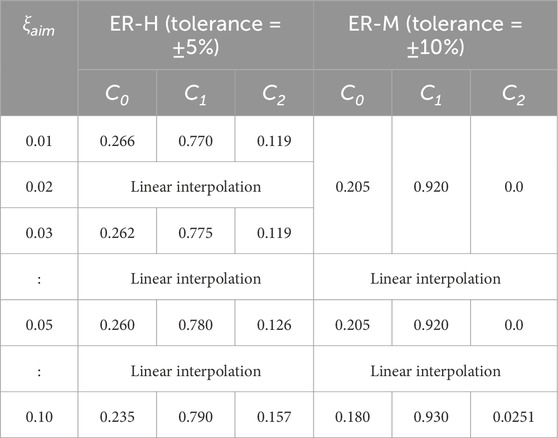
Table 3. Coefficients C₀–C₂ for ER.

Figure 8

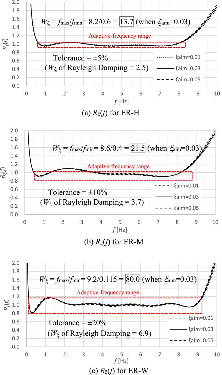
Figure 8. Comparison of W_ξ of the ER models. (A) R_ξ(F) for ER-H (B) R_ξ(F) for ER-M (C) R_ξ(F) for ER-W.

f_min, f_max and W_ξ for ER-H and ER-M are presented in Table 4. The W_ξ value for each model ranged within 13.5–13.7 and 21.3–21.5 for ξ_aim = 0.01–0.05.

Table 4

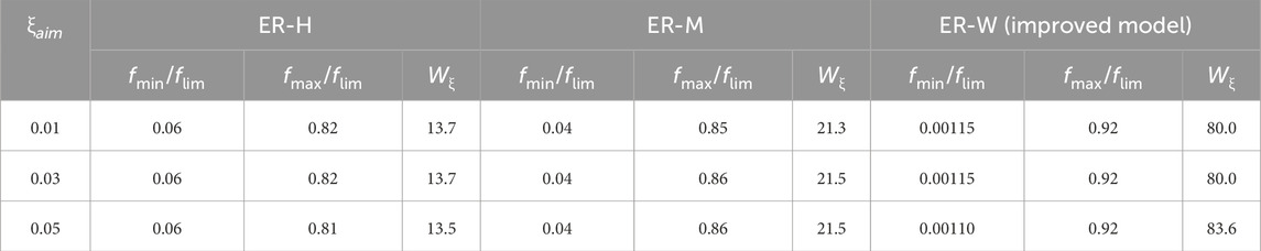
Table 4. Comparison of the adaptive-frequency range for ER.

4 Improvement for a wider adaptive-frequency range

In Section 3, CH9, ER-H, and ER-M models were introduced. Although these models achieve higher W_ξ values than Rayleigh damping, they fall short of meeting the target W_ξ of over 50. Therefore, we first improve the causal hysteresis damping to achieve W_ξ = 50 with a tolerance below 15% (CH19). Next, we aim to develop a model with an even larger W_ξ using extended Rayleigh damping, achieving W_ξ = 80 with a tolerance below 20% (ER-W).

4.1 Causal damping model with N = 19 (CH19)

In the causal damping model, we previously used a model (CH9) with a time delay term (N) of 9, which proved insufficient. Therefore, we consider a model (CH19) in which N is increased to 19. Although this expansion improves W_ξ, the increased N in time–history response analysis may reduce computational efficiency. Table 5 shows the coefficients (b₁-b₁₉) for CH19, with Δt(s) and a₀ remaining the same as in Table 2. Figure 8B shows R_ξ of CH19. The overall trend is similar to CH9, but with a larger W_ξ of 57.4 when ξ_aim = 0.03. The peak appears around 0.8 Hz for CH9 and shifts to around 0.4 Hz for CH19, with each model’s maximum tolerance corresponding to these peaks.

Table 5

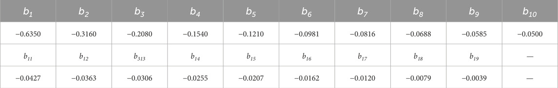
Table 5. Coefficients for CH19.

Table 6 compares the tolerances and W_ξ values of CH9 and CH19 for the same ξ_aim. Higher ξ_aim generally results in a larger tolerance. When ξ_aim = 0.03, the tolerance is 11% with W_ξ = 25.8 for CH9, whereas for CH19, the tolerance slightly increases to 14%, but W_ξ reaches 57.4. For CH19, W_ξ exceeds 50 across all cases, when ξ_aim ranges between 1% and 5%.

Table 6

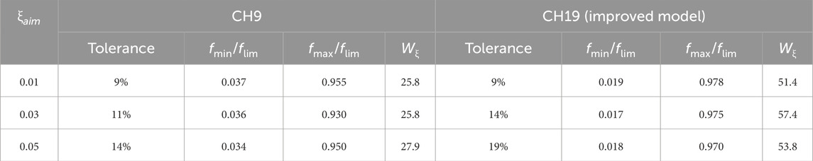
Table 6. Comparison of the adaptive-frequency range for CH9 and CH19.

In addition, when using the proposed model, the setting of F_lim is important, it is necessary to give F_lim so that the frequency range to be considered falls between F_min and F_max referring to Table 6.

4.2 Extended Rayleigh damping model for a wider adaptive area (ER-W)

We propose the ER-W model, designed to expand W_ξ with a slight trade-off in accuracy. The target damping ratio, ξ_aim, is set within the range of 0.005–0.05, with an allowable tolerance of ±20% in the adaptive-frequency range. This model employs a four-term CH model, defined by coefficients a₀ and b₁–b_4, since a two-term CH model cannot achieve that performance. Equations 10, 11 show the calculation method for this model, which is simpler than ER-H and ER-M due to its broader tolerance. This model is called ER-W for its wider adaptive area. R_ξ is calculated by Equation 9 as above.

The coefficient α₀' in Equation 11 was optimized through numerical trials within the range 0.005 < ξ_aim < 0.05 within the ±20% tolerance. This optimization resulted in dividing ξ_aim into two groups, above and below 0.02, since a single α₀' value could not be applied across all ξ_aim. Figure 8C displays the R_ξ values for ER-W with f_lim set at 10 Hz, while Table 4 compares the W_ξ values of ER-W against those of ER-H and ER-M. For 0.01 < ξ_aim ≤ 0.05, the W_ξ of the ER-W model exceeds 80. However, ER-W shows significant fluctuations in the low-frequency range, resulting in comparatively lower accuracy in that range.

As mentioned above, when using the proposed model, the setting of F_lim is important, it is necessary to give F_lim so that the frequency range to be considered falls between F_min and F_max referring to Table 4.

Although this model achieves a larger W_ξ than CH19, being a type of Rayleigh damping model, it still faces limitations—such as issues in models with rigid body motion (e.g., uplift or sliding)—as described by Hall (2006).

$\left\{D\left(t\right)\right\}=\left({{\alpha }_0}^{\prime }\left[M\right]+{{\alpha }_1}^{\prime }\left[K\right]\right)\left\{\dot{u}\left(t\right)\right\}+2{\xi }_{aim}\cdot \left[K\right]\cdot \left({\displaystyle \sum _{j=1}^4}{b}_j\left\{u\left(t-j\cdot t_{\lim }\right)\right\}\right)(10)$

Here,

$\left.\begin{array}{l}{{\alpha }_0}^{\prime }=\left(0.1445{\xi }_{aim}+2.513\times {10}^{-5}\right)f_{\lim }\left(0.005\le {\xi }_{aim}<0.02\right)\\ {{\alpha }_0}^{\prime }=\left(0.1376{\xi }_{aim}+17.59\times {10}^{-5}\right)f_{\lim }\left(0.02\le {\xi }_{aim}\le 0.05\right)\\ {{\alpha }_1}^{\prime }=2{\xi }_{aim}{a}_0,a_0=1/\left(\pi \cdot f_{\lim }\right)\\ b_1=-0.616,b_2=-0.275,b_3=-0.145b_4=-0.065,t_{\lim }=1/f_{\lim }\left(s\right)\\ {\xi }^{\prime }\left(f\right)\approx \frac{{{\alpha }_0}^{\prime }}{4\pi f}+\frac{{\xi }_{aim}{Z}_{I4}^{\prime }\left(f\right)}{1+2{\xi }_{aim}{Z}_{R4}^{\prime }\left(f\right)}\\ Where{Z}_{R4}^{\prime }\left(f\right)={\displaystyle \sum _{j=1}^4}{b}_j\cos \left(2j\pi f\Delta t\right),Z_{I4}^{\prime }\left(f\right)=a_0-{\displaystyle \sum _{j=1}^4}{b}_j\sin \left(2j\pi f\Delta t\right)\end{array}\right\}(11)$

5 Analysis of a high-rise steel building

To compare the properties of various damping models, we conducted horizontal and vertical simultaneous input analysis on a 35-story high-rise steel building, following the approach used by Mogi et al. (2023). To directly evaluate beam vibrations, a long beam was divided into small elements, generating localized vibrational beam modes, and the response in the long beam was then calculated. The columns were assigned elastic properties with bilinear hysteresis at both ends. The model includes 756 nodes and 1756 DOF.

Figure 9 shows the element division of the building’s analytical model. In the horizontal direction, the first three mode frequencies are 0.21 Hz, 0.62 Hz, and 1.08 Hz. Figure 10 shows the effective mass ratio for each mode, with the first mode accounting for 77% in the horizontal direction and surpassing 90% by the third mode. Therefore, first to third modes are important for the horizontal response evaluation.

Figure 9

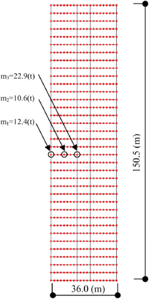
Figure 9. Modeling image of the analyzed steel building.

Figure 10

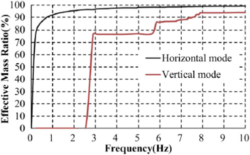
Figure 10. Effective mass ratio of the building.

The first vertical mode corresponds to the overall seventh mode, at 2.9 Hz. Vertical modes differ from horizontal ones and are distributed across a broad frequency range. Overall 7th–12th modes (2.9–4.9 Hz) are column vibration modes, arising from column compression and tension, while the overall 15th–40th modes (5.8–7.2 Hz) represent prominent local beam vibrations. The effective mass ratio in the vertical direction reaches nearly 90% up to the 40th mode. Consequently, to evaluate beam response behavior, modes up to the 40th must be represented, necessitating a minimum W_ξ of 36 (7.2(Hz)/0.2(Hz)). However, to accommodate more complex cases, we set a target W_ξ of 50. In addition to the WP model used as a benchmark, we employed Rayleigh damping, widely used in practice, along with CH9, ER-H, ER-M and the proposed CH19 and ER-W models. Uniform damping models UN0 and UN1 were also studied as outlined in Section 3.1.

Figure 11 shows the accuracy of the damping ratio R_ξ for each model. R_ξ is the ratio of the calculated damping ratio ξ(f) at each frequency to the target damping ratio ξ_aim (set at 0.02 in this case). The ξ(f) values were calculated from the logarithmic decay characteristics of 100 single-DOF models with natural frequencies between 0.01 and 10 Hz using each damping model. CH-9 and CH-19 are almost the same as the theoretical characteristics of the causal damping model (Figure 7), while ER-H, ER-M and ER-W correspond well to the theoretical extended Rayleigh damping model (Figure 8).

Figure 11

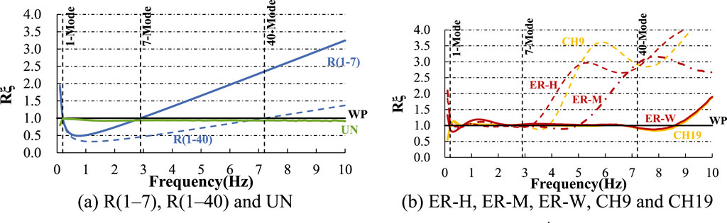
Figure 11. Accuracy of the damping ratio R_ξ = ξ(F) ∕ ξ_aim. (A) R (1–7), R (1–40) and UN (B) ER-H, ER-M, ER-W, CH9 and CH19.

Rayleigh damping is tested in two configurations: where the target damping ratio applies to the first and seventh modes [labeled R (1–7)], primarily for horizontal modes, and another for the 1st and 40th modes [named R (1–40)], for both horizontal and vertical modes. The f_lim for ER-H, ER-M, and ER-W was set at 4.0, 6.0, and 15.0 Hz, respectively. As shown in Figure 11, the upper accuracy limits for ER-H and ER-M are approximately 3.5 and 5 Hz, respectively, while ER-W surpasses the 7.2 Hz target frequency. The f_lim for CH9 and CH19 were set to 4.5 and 10.0 Hz, respectively, with CH19 also exceeding 7.2 Hz.

We applied two types of seismic motion inputs: L1 (once-every-50-year event scaled by 0.2) and L2 (once-every-500-year event scaled by 1.0). The seismic motions were input simultaneously in the horizontal and vertical directions. For L1, all members remained within the elastic range, while for L2, the beams entered the plastic range, though columns stayed elastic. Figure 12 shows the acceleration and displacement response spectra for L2 seismic motion, with the damping ratio set at 0.02.

Figure 12

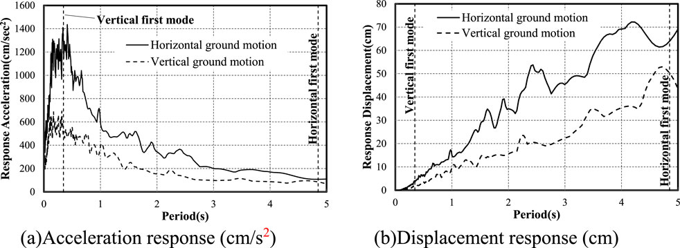
Figure 12. Simulated earthquake motion. (A) Acceleration response (cm/s²) (B) Displacement response (cm).

The Newmark-β method (β = 1/4) was used for time integration. For R and ER models, the integration time interval was set to Δt = 0.01 s. For WP, Δt = 0.005 (s) was used because it diverged at Δt = 0.01 (s). Since UN1 requires fine time increments for solution stability, its integration time interval was set to Δt = 0.0005 (s) based on preliminary trials.

6 Results and discussion

Figures 13, 14 illustrate the elastic peak response result at a scale factor of 0.2 (L1 earthquake), while Figures 15, 16 present the inelastic peak response result at a scale factor 1.0 (L2 earthquake). The beam amplitude was derived by calculating difference between the nodal vertical displacement at the center of the long-span beam and average vertical displacement of the nodes at both ends. Vertical acceleration represents vertical response at the center node of the long-span beam. Shear coefficient was determined by dividing the story shear force at each story by the weight above it. In addition, side column axial force ratio graphically represents the ratio of the side column response of each damping model to that of the WP. In the nonlinear analysis, Rayleigh damping is applied in both the initial and tangent models, with the tangent model shown in all analysis results, including the ER model, due to minimal differences between the two.

Figure 13

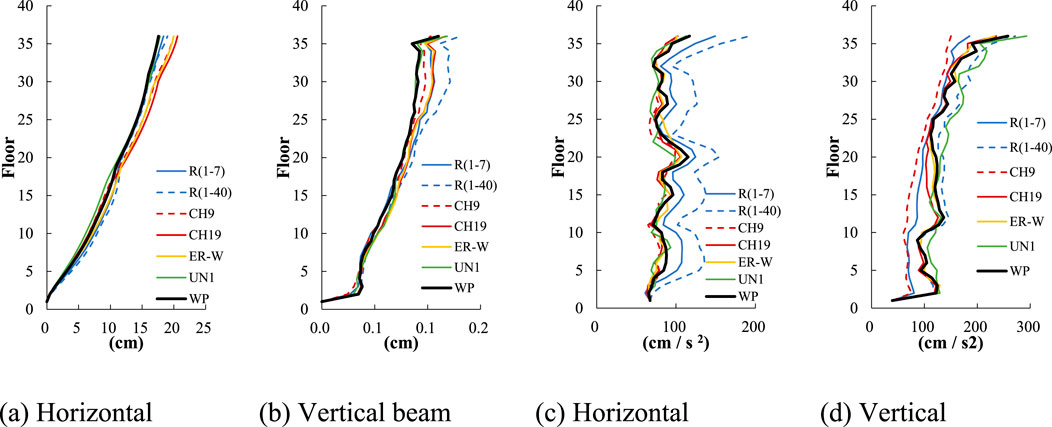
Figure 13. Distributions across the height of the 35-story building: (A) peak horizontal displacement at each floor, (B) peak beam vertical displacement at each floor, (C) peak horizontal acceleration at each floor and (D) peak vertical acceleration at each floor (L1 earthquake).

Figure 14

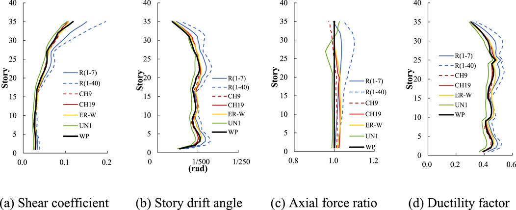
Figure 14. Distributions across the height of the 35-story building: (A) peak shear coefficient in each story, (B) peak story drift angle in each story, (C) peak axial force ratio in each story and (D) ductility factor in each story (L1 earthquake).

Figure 15

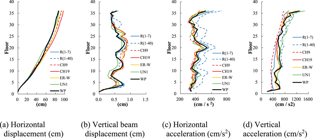
Figure 15. Distributions across the height of the 35-story building: (A) peak horizontal displacement at each floor, (B) peak beam vertical displacement at each floor, (C) peak horizontal acceleration at each floor and (D) peak vertical acceleration at each floor (L2 earthquake).

Figure 16

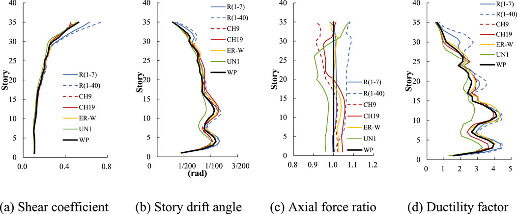
Figure 16. Distributions across the height of the 35-story building: (A) peak shear coefficient in each story, (B) peak story drift angle in each story, (C) peak axial force ratio in each story and (D) ductility factor in each story (L2 earthquake).

In all figures, the results of R (1–7) and R (1–40) are shown as current general methods, with WP included as the benchmark method for comparison. In addition, the models CH9, CH19, ER-W, and UN1 are also described in these figures. As shown in Figure 11, CH9, ER-H, and ER-M cannot capture modes beyond the seventh mode (2.9 Hz), resulting in less accurate analysis outcomes. Therefore, only CH9 is retained as a representative of this group. CH19 and ER-W represent the proposed methods, while the modified method (UN1) is displayed among the uniform damping methods for its superior accuracy over the original method (UN0).

Figure 13A shows the horizontal displacement, where nearly all models align well with WP due to the predominance of the first-order mode, though CH19 and ER-W show slightly larger values, a phenomenon discussed later. In Figure 13B, the beam amplitude shows a more substantial discrepancy in R (1–40) compared to other models, attributed to an underestimation of the damping ratio from the 2nd to 40th order. This discrepancy more pronounced in Figure 13C for horizontal acceleration, where both R (1–40) but also R (1–7) exhibit larger responses. For vertical acceleration in Figure 13D, the influence of the 40th order mode at 7.2 Hz is significant, CH9 and R (1–7) show a marked difference from WP due to its inability to accommodate the damping ratio of this mode. Throughout Figure 13, UN1 delivers an accurate response, and the proposed ER-W and CH19 also perform well.

The shear coefficient in Figure 14A and story drift angle in Figure 14B reveal larger responses for R (1–7) and R (1–40) relative to WP, possibly due to these models underestimating damping for the first–seventh orders. On the other hand, other models generally perform well, but UN1 shows a slightly lower response. Although not displayed, UN0 is even less accurate, especially in Figure 14B; while the UN1 modification improves accuracy, slight differences persist. Figure 14C shows the ratio of the column axial force across all layers, with R (1–40) displaying a larger response due to its underestimation of damping across modes. The ductility factor of all models in Figure 14D is smaller than 1, reflecting an elastic range analysis. And all models exhibit properties similar to those seen in Figure 14B.

Figures 15, 16 display results for the nonlinear range, with trends similar to those in Figures 13, 14 for the elastic range. In Figure 15A, CH19 and ER-W exhibit slightly larger results than WP, while other models show minimal deviation from WP, consistent with Figure 3. In Figures 15B–D, UN1 and the proposed ER-W and CH19 correspond WP.

In Figures 16A, B, deviations from WP are observed for R (1–7), R (1–40), while other models align closely. The difference between UN1 and WP is reduced compared to Figure 14. In Figure 16C, all models diverge from WP, but R (1–7) is the closest. In Figure 16D, results mirror those in Figure 16B, with CH9, CH19, and ER-W showing strong correspondence to WP, though deviations are more pronounced.

Through Figures 13–16, it can be observed that the proposed CH19 and ER-W models provide better responses, as compared to Rayleigh damping. However, the horizontal displacements of these models, dominated primarily by first-order modes, tend to be larger, with ratios relative to WP at the top of the building reaching 1.17 for CH19 and 1.14 for ER-W in the linear analysis (L1 earthquake) as shown in Figure 13A. In the nonlinear analysis (L2 earthquake), these differences are slightly reduced, with CH19 and ER-W at 1.12 and 1.06, respectively (Figure 15A).

Figure 17 shows the accuracy R_f(f) of the resonance frequencies of CH19 and ER-W models with ξ = 0.02, as used in the analysis. R_f(f) is expressed as the product of stiffness accuracy R_fk(f) and the damping accuracy R_fξ(f), as shown in Equation 12.

$\left.\begin{array}{l}{R}_f\left(f\right)=R_{fk}\left(f\right)\cdot R_{f\xi }\left(f\right)\\ where{R}_{fk}\left(f\right)=\sqrt{1+2{\xi }_{aim}\cdot Z_R^{\prime }\left(f\right)},R_{f\xi }\left(f\right)=\sqrt{\frac{1-\xi {\left(f\right)}^2}{1-{{\xi }_{aim}}^2}}\end{array}\right\}(12)$

Figure 17

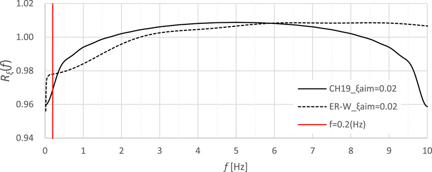
Figure 17. Frequency variation of the first-order mode for CH19 and ER-W.

With the f_lim set at 10 Hz for CH19 and 15 Hz for ER-W, Figure 17 plots from 0 Hz to 10 Hz on the abscissa. The first-order analysis frequency of 0.2 Hz is also shown in the figure. The R_f (0.2) values for CH19 and ER-W are 0.969 and 0.978, respectively, corresponding to first-order resonance frequencies of 1.94 and 0.196 Hz. This deviation from the original first-order mode frequency of 0.2 Hz is considered to have changed the seismic input component, contributing to the observed differences in the first-order mode response.

7 Calculation load

Table 7 presents the computation times for each damping model. Models R (1–7), R (1–40), ER-H, ER-W, CH9, and CH19 showed stable and accurate performance even with a relatively coarse time increment (0.01 s). In contrast, UN0 and UN1 required considerably more CPU time, due to the need for fine integration time intervals (0.0005 s) to maintain stability. WP, as a dense matrix, incurs a high computational cost for the Cholesky decomposition of effective stiffness matrix K ∼.

Table 7

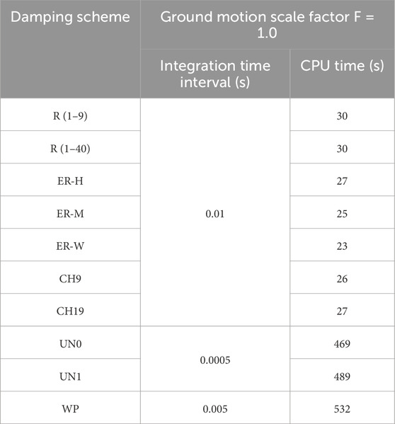
Table 7. CPU times spent on computations.

All analyses were carried out on an SD530 Lenovo Think System equipped with an Intel Xeon Gold 6,246 3.3 GHz CPU. Analyzing the WP model required 532 (s), while uniform damping required a time step of 0.0005 (s), resulting in a calculation time of 469 (s). Models R (1–7) and R (1–40) completed in 30 (s), while ER-H and ER-M took 27 (s) each. The proposed ER-W and CH19 required 23 (s) and 27 (s), respectively, making their computational loads comparable to standard Rayleigh damping. Although UN1 achieves high analysis accuracy, its implicit method demands finer time increments, extending the duration of the analysis. This computational burden is likely to increase substantially for larger analytical models.

8 Conclusion

In the seismic response analysis of the large-scale models, which will become increasingly important in the future, there is a need for a damping model that can maintain a consistent damping ratio from low- to high-order modes, with minimal computational load. In the current seismic design, Rayleigh damping is commonly applied in seismic design for such cases; however, its frequency range for achieving a constant damping ratio is considerably narrow. In this study, we define this frequency range using the coefficient W_ξ, and propose a damping model suited for scenarios where W_ξ exceeds 50.

For standard Rayleigh damping, W_ξ is relatively low, approximately 3.7 with a 10% tolerance and approximately 6.9 with a 20% tolerance. In contrast, the causal damping and modified Rayleigh damping models we have previously proposed achieve W_ξ values of 26 and 21, respectively, at a 10% tolerance. While sufficient for many applications, the high-rise model examined here includes local beam vibration modes in addition to horizontal and vertical modes, necessitating new damping models with W_ξ values of 36. However, to accommodate more complex cases, we set a target W_ξ of 50.

Therefore, we first improved causal hysteresis damping, achieving a W_ξ of 50 with a 15% tolerance. We then ER damping to attain a larger W_ξ, reaching 80 with a 20% tolerance. These models were applied to both linear and nonlinear seismic response analyses of a steel-framed high-rise structure, demonstrating high accuracy with computation times similar to those of standard Rayleigh damping, thereby confirming the efficacy of the proposed models.

In many of the problems that have been studied so far, the input seismic motion was assumed to be either horizontal or vertical. In such cases, the conventional model of W_ξ was sufficient to cover the required frequency range. However, for analyses that assume simultaneous horizontal and vertical inputs, as in the example in this study, and that also consider local vibration modes, the conventional model of W_ξ is not sufficient. The model proposed in this paper is effective for such problems.

As for the application of these damping models, although the example was a 2-dimensional model, it is also possible that a 3-dimensional model will be used in the future. In that case, the model will be even larger, so the models proposed in this paper will be even more effective. In addition to this, for example, in an analysis where the same 3 directions of input as the actual phenomenon are applied to a large-scale 3-dimensional FE model of a nuclear power plant building, we believe that the effectiveness of the models will be even more apparent.

For future development of these models, several issues are noteworthy. First, in both models, the damping ratio variation is relatively high near the lower limit (f_min) of the applicable range. It is desirable to achieve a more stable damping ratio in this range. In addition, it is necessary to consider how to deal with cases where a larger W_ξ is required.

For causal history damping, the model currently requires 19 past displacements, which could be optimized by reducing this count to improve calculation efficiency for larger analysis model. Although ER damping achieves a high W_ξ, it remains a variant of Rayleigh damping, thus retaining some inherent limitations such as issues with rigid body motion, making it challenging to apply in specific cases. Therefore, evaluating each model’s applicability based on many problems is essential.

Data availability statement

The raw data supporting the conclusions of this article will be made available by the authors, without undue reservation.

Author contributions

NN: Writing–original draft, Writing–review and editing. YM: Writing–review and editing. AO: Writing–review and editing. KN: Writing–review and editing.

Funding

The author(s) declare that financial support was received for the research, authorship, and/or publication of this article. This study was supported by JSPS KAKENHI Grant Number JP22H01645. The authors have no financial conflicts of interest to disclose concerning the study.

Conflict of interest

Author YM was employed by Taisei Corporation. Author AO was employed by Taisei Corporation.

The remaining authors declare that the research was conducted in the absence of any commercial or financial relationships that could be construed as a potential conflict of interest.

Publisher’s note

All claims expressed in this article are solely those of the authors and do not necessarily represent those of their affiliated organizations, or those of the publisher, the editors and the reviewers. Any product that may be evaluated in this article, or claim that may be made by its manufacturer, is not guaranteed or endorsed by the publisher.

References

Chopra, A. K., and McKenna, F. (2016). Modeling viscous damping in nonlinear response history analysis of buildings for earthquake excitation. Earthq. Eng. and Struct. Dyn. 45 (2), 193–211. doi:10.1002/eqe.2622

CrossRef Full Text | Google Scholar

Hall, J. F. (2006). Problems encountered from the use (or misuse) of Rayleigh damping. Earthq. Eng. and Struct. Dyn. 35 (5), 525–545. doi:10.1002/eqe.541

CrossRef Full Text | Google Scholar

Huang, Y., Sturt, R., and Willford, M. (2019). A damping model for nonlinear dynamic analysis providing uniform damping over a frequency range. Comput. and Struct. 212 (C), 101–109. doi:10.1016/j.compstruc.2018.10.016

CrossRef Full Text | Google Scholar

Ichihara, Y., Nakamura, N., Moritani, H., Choi, B., and Nishida, A. (2021). 3D FEM soil-structure interaction analysis for kashiwazaki - kariwa nuclear power plant considering soil separation and sliding. Front. Built Environ. 7. doi:10.3389/fbuil.2021.676408

CrossRef Full Text | Google Scholar

Inaudi, J. A., and Kelly, J. M. (1995). Linear hysteretic damping and the Hilbert transform. J. Eng. Mech. 121 (5), 626–632. doi:10.1061/(asce)0733-9399(1995)121:5(626)

CrossRef Full Text | Google Scholar

Jehel, P., Legar, P., and Ibrahimbegovic, A. (2014). Initial versus tangent-stiffness based Rayleigh damping in inelastic time history analysis. Earthq. Eng. and Struct. Dyn. 43, 467–484. doi:10.1002/eqe.2357

CrossRef Full Text | Google Scholar

Kinoshita, T., Nakamura, N., and Kashima, T. (2021). Characteristics of the first-mode vertical vibration of buildings based on earthquake observation records. Jpn. Archit. Rev. 4 (2), 290–301. doi:10.1002/2475-8876.12208

CrossRef Full Text | Google Scholar

Kitayama, S., and Constantinou, M. (2022). Effect of modeling of inherent damping on the response and collapse performance of seismically isolated buildings. Earthq. Eng. Struct. Dyn. 52 (3), 571–592. doi:10.1002/eqe.3773

CrossRef Full Text | Google Scholar

Lee, C. L. (2021). Bell-shaped proportional viscous damping models with adjustable frequency bandwidth. Comput. and Struct. 244, 106423. doi:10.1016/j.compstruc.2020.106423

CrossRef Full Text | Google Scholar

Livermore Software Technology Corporation (2021). LS-DYNA keyword user’s manual. An ANSYS Co. 1 (R13.0). Available at: https://www.dynasupport.com/manuals.

Google Scholar

Mogi, Y., Nakamura, N., Nabeshima, K., and Ota, A. (2022). Vibration characteristics of capped viscous damping based on frame restoring-force amplitude. Front. Built Environ. 8. doi:10.3389/fbuil.2022.858029

CrossRef Full Text | Google Scholar

Mogi, Y., Nakamura, N., Nabeshima, K., and Ota, A. (2023). Performance of inherent damping models in inelastic seismic analysis for tall building subject to simultaneous horizontal and vertical seismic motion. Earthq. Eng. and Struct. Dyn. 52 (12), 3746–3764. doi:10.1002/eqe.3946

CrossRef Full Text | Google Scholar

Nakamura, N. (2007). Practical causal hysteretic damping. Earthq. Eng. and Struct. Dyn. 36 (5), 597–617. doi:10.1002/eqe.644

CrossRef Full Text | Google Scholar

Nakamura, N. (2016). Extended Rayleigh damping model. Front. Built Environ. 2. doi:10.3389/fbuil.2016.00014

CrossRef Full Text | Google Scholar

Nakamura, N., Kinoshita, T., and Fukuyama, T. H. (2017). Response analysis and auto-regressive exogenous modeling of a steel-reinforced concrete high-rise building during the 2011 off the pacific coast of tohoku earthquake. Front. Built Environ. 3. doi:10.3389/fbuil.2017.00074

PubMed Abstract | CrossRef Full Text | Google Scholar

Nakamura, N., Nabeshima, K., Mogi, Y., and Ota, A. (2023). Nonlinear earthquake response analysis using causal hysteretic damping and extended Rayleigh damping, Eurodyn2023. Netherland: Delft.

Google Scholar

Ota, A., Nakamura, N., Nabeshima, K., Mogi, Y., and Kawabata, M. (2023). Fundamental study of damping models with enhanced frequency Independence in nonlinear seismic response analysis comparison of causality -based damping and uniform damping models. J. Struct. and Constr. Eng. 88 (811), 1348–1359. (in Japanese). doi:10.3130/aijs.88.1348

CrossRef Full Text | Google Scholar

Tian, Y., Fei, Y., Huang, Y., and Lu, X. A. (2022). A universal rate-dependent damping model for arbitrary damping-frequency distribution. Eng. Struct. 255, 113894. doi:10.1016/j.engstruct.2022.113894

CrossRef Full Text | Google Scholar

Tian, Y., Huang, Y., Qub, Z., Feic, Y., and Lua, X. (2023). High-performance uniform damping model for response history analysis in OpenSees. J. Earthq. Eng. 27 (Issue 11), 3136–3152. doi:10.1080/13632469.2022.2124557

CrossRef Full Text | Google Scholar

Wilson, E. L., and Penzien, J. (1972). Evaluation of orthogonal damping matrices. Int. J. Numer. Methods Eng. 4 (1), 5–10. doi:10.1002/nme.1620040103

CrossRef Full Text | Google Scholar

Wu, Z., Wei, L., and Ikago, K. (2023). Feasibility study of a practical causal rate-independent damping device for the improved performance of seismic isolated structures. Eng. Struct. 275, 15. doi:10.1016/j.engstruct.2022.115305

CrossRef Full Text | Google Scholar