Adaptive sliding-mode delay compensation for real-time hybrid simulations with multiple actuators

Real-time hybrid simulation (RTHS) is a widely applied test method in structural engineering, which is developed from pseudo-dynamic test. Much of the past work has been centered on one-dimensional RTHS using a single hydraulic actuator. When the complexity of the problem demands to increase the number of degrees of freedom to be enforced on the boundary conditions, more than one hydraulic actuator must be used. Multiple-actuator or multi-axial RTHS (maRTHS) requires that more than one hydraulic actuator exerts the required motion on experimental substructures demanding the implementation of multiple-input multiple-output (MIMO) control strategies. A new maRTHS benchmark control problem has been developed, focusing on a frame subjected to seismic load at the base, substantially transforming and intensifying the complexity of the problem. The time delay generated by the dynamic characteristics of the loading system and the transmission process as well as the high coupling between the hydraulic actuators and the nonlinear kinematics escalates the complexity of the actuator control tracking. A sliding mode adaptive delay compensation method suitable for maRTHS is proposed, which utilizes a MIMO sliding mode method to reduce the coupling effects of actuators and the adaptive compensation method to compensate the residual delay. The effectiveness of the method is verified by numerical simulating different working conditions in the Benchmark Problem Platform.

1 Introduction

In recent years, the application of real-time hybrid simulation (RTHS) has become increasingly widespread in civil and other engineering (Stoten et al., 2016; Jiang et al., 2020; Liu, 2020; Yang et al., 2020). It divides the overall structure into numerically simulated substructures and experimentally loaded test substructures, combines real-time loading of physical specimens with computer numerical calculations. It requires the realization of boundary coordination between substructures, namely, force balance and deformation coordination at substructure boundaries. Therefore, substructure boundary coordination becomes critical to the success of RTHS (Horiuchi et al., 1999; Gao, 2012).

RTHS requires the experimental loading and data transmission to the numerical substructure in real-time, thus system delays will significantly affect the accuracy and stability of RTHS (Gao et al., 2013b). Additionally, the interactions between loading equipment and experimental substructure during tests will lead to the variations of the time delays. Therefore, the development of adaptive time delay compensation methods has been pursued to ensure the stability and precision of RTHS (Wallace et al., 2005; Philips and Spencer, 2011; Chen et al., 2012; Chae et al., 2013; Wu et al., 2013; Ou et al., 2015; Salvatore and Mario, 2016; Hayati and Song, 2017; Zhou et al., 2017; Chae et al., 2018; Alejandro and Mariantonieta, 2019; Wang et al., 2019; Zhou et al., 2019; Wang et al., 2020; Ning et al., 2023). Wang et al. (2019) proposes an adaptive Kalman-based noise filter and an adaptive two-stage delay compensation method, which achieves outstanding tracking performance and excellent robustness. Ning et al. (2023) added a feedback controller to the adaptive feedforward controller to reduce the dependency on the ADM method. Results of virtual and actual RTHS alongside five other compensation strategies revealed the superiority of the proposed compensation method. Wang et al. (2020) proposes an adaptive delay compensation method based on a discrete model (ADM) of the loading system. On the other side, nonlinear control methods especially sliding mode control (SMC) was used to improve the control accuracy (Wu and Zhou, 2014; Rajabi et al., 2018; Xu et al., 2019; Yang et al., 2021; Yang et al., 2023). Wu and Zhou (Wu and Zhou, 2014) used SMC in RTHS for single degree of freedom structure, incorporating the “internal model design” approach into the controller to enable asymptotic tracking of various reference input signals with zero steady-state error. Xu et al. (2019) combined SMC method with improved adaptive polynomial-based forward prediction to improve the robustness of RTHS system. Yang et al. (Yang et al., 2021; Yang et al., 2023) applied the slide mode control in acceleration control for shaking table test and shake table real-time hybrid simulation. Rajabi et al. (2018) combined slide mode control with online state estimations using EKF/UKF to control the shaking table. These adaptive time delay compensation methods and sliding mode control methods are mainly developed for single degree of freedom test, their control effects for maRTHS need to be studied.

Addressing the coupling effects through the intuitive approach of individually compensating for the dynamic characteristics of each actuator may not be very effective. Therefore, a control algorithm tailored for multi-input-multi-output (MIMO) systems is essential in the context of collaborative loading in hybrid tests with multiple actuators. With the development of RTHS, the experimental substructures have become increasingly complex, often exhibiting strong non-linearity and multiple degrees of freedom characteristics. This necessitates the conduct of multi-directional control and delay compensation in RTHS (Gao et al., 2013a; Fermandois and Spencer, 2017; Sarebanha et al., 2019; Najafi and Spencer, 2021; Tian et al., 2022; Najafi et al., 2023). Fermandois and Spencer (Fermandois and Spencer, 2017) proposed model-based framework control method for multi-axial real-time hybrid simulation testing. Najafi et al. (Najafi and Spencer, 2021; Najafi et al., 2023) proposed a multi-axial real-time hybrid simulation framework that could achieve decoupling control for six actuators. This framework was applied to a small-scale specimen, which must be verified on a full-scale specimen. Tian et al. (2022) proposed an enhanced three variable control method to trace high-frequency force signals of a multi-degree-of-freedom (MDOF) boundary coordinating device. Sarebanha et al. (2019) applied adaptive time series compensator for real-time hybrid simulation of seismically isolated structures in three degree of freedom. Gao et al. (2013a) developed generalized robustness control procedure for MDOF real-time hybrid simulation. For such tests involving multiple actuators for cooperative control, there exists coupling between multiple actuators at the same control point. This means that during the control process of multiple degrees of freedom, a controlled quantity is influenced by multiple control variables. The presence of this coupling effects result in the response of a particular degree of freedom being influenced by multiple actuators, creating mutual interactions among different control points through the test specimen. When this coupling effects of actuators is strong and the load capacity of actuators is limited, it significantly diminishes the tracking control effectiveness of the actuators. Consequently, it becomes challenging to ensure boundary coordination between substructures, leading to a reduction in experimental accuracy and even test failure.

In response to the coupling issue arising from the collaborative loading of multiple actuators in RTHS, this paper develops a sliding mode adaptive time-delay compensation method applicable to MDOF loading. Expanding the single-degree-of-freedom sliding mode control method into vector form to accommodate MIMO systems, the MDOF sliding mode control (MSMC) method is employed to reduce or even eliminate coupling effects of actuators, achieving similar effects to decoupling. Since the parameters of the sliding mode controller are fixed once set and cannot adaptively adjust their gains based on actual states, to optimize the compensation algorithm, allowing the controller to adaptively adjust its parameters based on operating conditions and responses, this paper integrates the ADM method for discrete model parameter identification with the MSMC method to reduce coupling effects of actuators. Based on the commands and feedback signals of the actuators, the model parameters are adaptively updated, and the controller gains are changed to reduce errors. Additionally, a distributed compensation strategy is adopted, applying ADM compensation to each degree of freedom’s sliding mode controller to address its residual delay, further enhancing the tracking control performance of the actuators.

This paper combines ADM and MSMC to propose a MDOF sliding mode adaptive time-delay compensation (ADM-MSMC) method suitable for maRTHS, aiming to enhance the robustness and accuracy of RTHS. In Section 2, the principles of the ADM-MSMC method are primarily introduced. Section 3 defines the benchmark control problem of maRTHS and presents the simulink diagram of the ADM-MSMC method based on the maRTHS Benchmark Problem Platform. Section 4 conducts RTHS of the proposed ADM-MSMC method based on the Benchmark Problem Platform to verify its feasibility and robust performance. The conclusions drawn from the numerical simulations are summarized in Section 5.

2 Adaptive sliding-mode delay compensation method with MDOF

In response to the issue of mutual coupling during simultaneous multi-actuator loading in RTHS, this section introduces an ADM-MSMC method suitable for MDOF loading. The SMC method is expanded into a vector form to accommodate MIMO systems. The MSMC method is employed to reduce or eliminate coupling effects of actuators, achieving similar effects to decoupling. Building upon this, a distributed compensation strategy is adopted, applying ADM method individually to each actuator to compensate for residual delay, further enhancing the tracking control performance of the actuators. Thus, this section first outlines the principles of the ADM-MSMC method, followed by separate explanations of the MSMC and ADM method.

2.1 ADM-MSMC method

The ADM-MSMC method adopts the MSMC method to reduce or eliminate the coupling effects of actuators of the MIMO system. On this basis, a decentralized compensation strategy is adopted, and the discrete model parameter identification ADM method compensates the residual delay of each actuator separately, which alleviates the difficulty of the method to compensate individually and achieves better tracking control effects. The principle of this method is shown in the following figure (taking a two-degree-of-freedom system as an example).

In Figure 1, the superscripts of the variables represent the different actuators. The parameter representation in Figure 1 is as shown in Equation 1:

${\mathbf{y}}_a=\left[{\mathrm{y}}_a^1{\mathrm{y}}_a^2\right],{\mathbf{y}}_{ac}={\left[y_{ac}^1{y}_{ac}^2\right]}^{\mathrm{T}},{\mathbf{y}}_c={\left[y_c^1{y}_c^2\right]}^{\mathrm{T}}={\mathit{k}}_1\mathbf{\xi }-\mathbf{K}\widehat{\mathbf{X}}{\mathbf{y}}_m=\left[{\mathrm{y}}_m^1{\mathrm{y}}_m^2\right],{\widehat{\mathbf{y}}}_m={\left[{\widehat{\mathbf{y}}}_m^1{\widehat{\mathbf{y}}}_m^2\right]}^{\mathrm{T}}\mathbf{e}={\mathbf{y}}_{ac}-{\widehat{\mathbf{y}}}_m,\mathbf{\xi }=\int \mathbf{e}\text{dt}(1)$

where: ${\mathbf{y}}_a$ is the target signal, ${\mathrm{y}}_a^i$ is the target signal of actuator i; ${\mathbf{y}}_{ac}$ is the actuator response signal, ${\mathrm{y}}_{ac}^i$ is the actuator i response signal; ${\mathbf{y}}_c$ is the compensated command vector of actuator, ${\mathrm{y}}_c^i$ is the compensated command of actuator i; ${\mathbf{y}}_m$ is the measured actuator output response vector, ${\mathrm{y}}_m^i$ is the measured actuator i output response; ${\widehat{\mathbf{y}}}_m$ is the observe response vector; ${\widehat{\mathrm{y}}}_m^i$ is the observe response of actuator i; ${\mathit{k}}_1$ refers to the integral gain coefficient; $\mathbf{K}$ represents the state feedback gain matrix; $\widehat{\mathbf{X}}$ is the observed state vector.

Figure 1

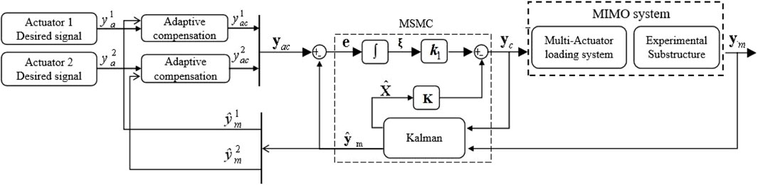
Figure 1. ADM-MSMC method block diagram.

2.2 MSMC method

SMC method is a discontinuous control method that introduces any initial state into a stable sliding surface in the phase plane. It allows the system, under certain conditions, to undergo small-amplitude, high-frequency oscillations along a specified state trajectory (the sliding surface), which is also the reason for its insensitivity to parameter variations. Generally, the design of sliding mode (abbreviated as sliding mode) control consists of the following two parts.

(1) Sliding surface design, which ensures that the system’s state trajectory exhibits asymptotically stable and other favorable dynamic characteristics after entering the sliding mode;

(2) Sliding mode control law design, which involves selecting different reaching laws to drive the system’s state trajectory onto the sliding surface within a finite time and maintain motion on it.

2.2.1 Sliding surface design

The SMC method first needs to determine the sliding surface. Let’s denote the spatial state equation of the controlled object as follows:

$\dot{\mathbf{Y}}\left(t\right)={\mathbf{A}}^{*}\mathbf{Y}\left(t\right)+{\mathbf{B}}^{*}\mathbf{u}(2)$

where $\mathbf{Y}\left(t\right)$ represents the state vector matrix. $\mathbf{u}$ is the input of the controlled system. Assuming the sliding surface is represented as $\mathbf{S}=\mathbf{\text{PY}}$, the sliding surface equation can be expressed as:

$\mathbf{S}=\mathbf{\text{PY}}=\mathbf{0}(3)$

Applying a linear transformation to the system’s state:

$\mathbf{\eta }=\mathbf{\Gamma }\mathbf{Y}(4)$

where $\mathrm{\Gamma }$ is the state transformation matrix, represented as:

$\mathbf{\Gamma }=\left[\begin{array}{c}{\mathbf{I}}_{\mathrm{n}}\\ \mathbf{0}\end{array}\begin{array}{c}{-\mathbf{B}}_1{\mathbf{B}}_2^{-1}\\ {\mathbf{I}}_{\mathrm{r}}\end{array}\right],{\mathbf{B}}^{*}=\left[\begin{array}{c}{\mathbf{B}}_1\\ {\mathbf{B}}_2\end{array}\right](5)$

In Equation 5, ${\mathbf{B}}_2$ is required to be non-singular; the number of elements in ${\mathbf{B}}_1$ and ${\mathbf{B}}_2$ are denoted by $n$ and $r$, respectively. Here, $n$ represents the number of deterministic or linear elements, while $r$ represents the number of uncertain or nonlinear elements. In the two-input-two-output servo-hydraulic system discussed in this chapter, $r$ = 2, and $n$ denotes the number of state vectors of the controlled object.

Substituting Equations 4, 5 into Equations 2, 3 respectively, one can derive the structural state equations and sliding surfaces denoted by $\dot{\mathbf{\eta }}$.

$\dot{\mathbf{\eta }}=\widehat{\mathbf{A}}\mathbf{\eta }+\widehat{\mathbf{B}}\mathbf{u}(6)$

$\mathbf{S}=\widehat{\mathbf{P}}\mathbf{Y}=\mathbf{0}(7)$

where: $\widehat{\mathbf{A}}=\mathbf{\Gamma }{\mathbf{A}}^{*}{\mathbf{\Gamma }}^{-\mathbf{1}};\widehat{\mathbf{B}}={\left[\mathbf{0},{\mathbf{B}}_2^{\mathrm{T}}\right]}^{\mathrm{T}};\widehat{\mathbf{P}}=\mathbf{P}{\mathbf{\Gamma }}^{-\mathbf{1}}$.

Decomposing Equations 6, 7 yields:

$\mathbf{\eta }=\left[\begin{array}{c}{\mathbf{\eta }}_1\\ {\mathbf{\eta }}_2\end{array}\right],\widehat{\mathbf{A}}=\left[\begin{array}{c}{\widehat{\mathbf{A}}}_{11}\\ {\widehat{\mathbf{A}}}_{21}\end{array}\begin{array}{c}{\widehat{\mathbf{A}}}_{12}\\ {\widehat{\mathbf{A}}}_{22}\end{array}\right],\widehat{\mathbf{P}}=\left[{\widehat{\mathbf{P}}}_1,{\widehat{\mathbf{P}}}_2\right](8)$

where ${\mathbf{\eta }}_1$ and ${\mathbf{\eta }}_2$ are $n\times r$ and $r\times r$ matrices respectively, while the dimensions of other matrices can be determined based on the dimensions of ${\mathbf{\eta }}_1$ and ${\mathbf{\eta }}_2$.

By Equations 6–8, we can obtain:

${\dot{\mathbf{\eta }}}_1={\widehat{\mathbf{A}}}_{11}{\mathbf{\eta }}_{\mathbf{1}}+{\widehat{\mathbf{A}}}_{12}{\mathbf{\eta }}_{\mathbf{2}}(9)$

$\mathbf{S}={\widehat{\mathbf{P}}}_1{\mathbf{\eta }}_{\mathbf{1}}+{\widehat{\mathbf{P}}}_2{\mathbf{\eta }}_{\mathbf{2}}=\mathbf{0}(10)$

For simplification of calculations, let ${\widehat{\mathbf{P}}}_2={\mathbf{I}}_{\mathrm{r}}$ be an identity matrix. From Equation 10, it follows that:

${\mathbf{\eta }}_{\mathbf{2}}=-{\widehat{\mathbf{P}}}_1{\mathbf{\eta }}_{\mathbf{1}}(11)$

Substituting Equation 11 into Equation 9, we can derive the nth-order motion equation for the system when it moves on the sliding surface as shown in Equation 12:

${\dot{\mathbf{\eta }}}_1=\left({\widehat{\mathbf{A}}}_{11}-{\widehat{\mathbf{A}}}_{12}{\widehat{\mathbf{P}}}_1\right){\mathbf{\eta }}_{\mathbf{1}}(12)$

Clearly, the design of the sliding surface $\mathbf{S}$ entails determining $\mathbf{P}$. If ${\widehat{\mathbf{P}}}_1$ can be reasonably determined to ensure the stability of the system’s motion on the sliding surface, and with ${\widehat{\mathbf{P}}}_2={\mathbf{I}}_{\mathrm{r}}$, the $\mathrm{P}$ matrix of the sliding surface can be determined. The principle of using the Linear Quadratic Regulator (LQR) method to determine the matrix $\mathbf{P}$ is to minimize the integral quadratic performance index of the state vector, as shown in Equation 13:

$J={\int }_0^{\mathbf{\infty }}{\mathbf{Y}}^{\mathrm{T}}\left(\mathrm{t}\right)\mathbf{\text{QY}}\left(\mathrm{t}\right)\text{dt}(13)$

where $\mathbf{Q}$ is a positive definite matrix. Substituting Equation 8 into the above equation, we obtain the objective function represented by $\mathbf{\eta }$ as shown in Equation 14:

$J={\int }_0^{\mathbf{\infty }}\left(\left[{\mathbf{\eta }}_1^{\mathrm{T}}{\mathbf{\eta }}_2^{\mathrm{T}}\right]\mathbf{T}\left[\begin{array}{c}{\mathbf{\eta }}_{\mathbf{1}}\\ {\mathbf{\eta }}_{\mathbf{2}}\end{array}\right]\right)\text{dt}(14)$

where the T is as shown in Equation 15:

$\mathbf{T}={\left({\mathbf{\Gamma }}^{-\mathbf{1}}\right)}^{\mathbf{T}}\mathbf{Q}{\mathbf{\Gamma }}^{-\mathbf{1}};\mathbf{T}=\left[\begin{array}{c}{\mathbf{T}}_{11}\\ {\mathbf{T}}_{21}\end{array}\begin{array}{c}{\mathbf{T}}_{12}\\ {\mathbf{T}}_{22}\end{array}\right](15)$

To minimize the objective function of Equation 14 while satisfying the motion equation constraints of Equation 9, according to the maximum principle, we can obtain ${\mathbf{\eta }}_{\mathbf{1}}$ with ${\mathbf{\eta }}_{\mathbf{2}}$ as the feedback state.

${\mathbf{\eta }}_{\mathbf{2}}=-0.5{\mathbf{T}}_{22}^{-1}\left({\widehat{\mathbf{A}}}_{12}^{\mathrm{T}}\mathbf{H}+2{\mathbf{T}}_{21}\right){\mathbf{\eta }}_{\mathbf{1}}(16)$

where $\mathbf{H}$ is the solution to the following Riccati Equation 17:

${\stackrel{\sim }{\mathbf{A}}}^{\mathrm{T}}\mathbf{H}+\mathbf{H}\stackrel{\sim }{\mathbf{A}}-0.5\mathbf{H}{\widehat{\mathbf{A}}}_{12}{\mathbf{T}}_{22}^{-1}{\widehat{\mathbf{A}}}_{12}^{\mathrm{T}}\mathbf{H}=-2\left({\mathbf{T}}_{11}-{\mathbf{T}}_{12}{\mathbf{T}}_{22}^{-1}{\mathbf{T}}_{12}^{\mathrm{T}}\right)\stackrel{\sim }{\mathbf{A}}={\widehat{\mathbf{A}}}_{11}-{\widehat{\mathbf{A}}}_{12}{\mathbf{T}}_{22}^{-1}{\mathbf{T}}_{21}(17)$

The well-known Riccati equation can be solved using the LQR function in MATLAB software to obtain the matrix $\mathbf{H}$. Combining Equations 11, 16, we get the Equation 18:

${\widehat{\mathbf{P}}}_1=0.5{\mathbf{T}}_{22}^{-1}\left({\widehat{\mathbf{A}}}_{12}^{\mathrm{T}}\mathbf{H}+{2\mathbf{T}}_{21}\right)(18)$

Considering Equation 8, we can get the Equation 19:

$\widehat{\mathbf{P}}=\left[{\widehat{\mathbf{P}}}_1{\widehat{\mathbf{P}}}_2\right]=\left[{\widehat{\mathbf{P}}}_1{\mathbf{I}}_{\mathrm{r}}\right](19)$

At this point, $\widehat{\mathbf{P}}$ is determined, and the matrix $\mathbf{P}=\widehat{\mathbf{P}}\mathbf{\Gamma }$ of the slip surface is also determined.

2.2.2 Sliding mode control law design

Using the Lyapunov method directly, the sliding mode control law is designed. Let the Lyapunov function be denoted as:

$v=0.5{\mathbf{S}}^{\mathrm{T}}\mathbf{S}=0.5{\mathbf{Y}}^{\mathrm{T}}{\mathbf{P}}^{\mathrm{T}}\mathbf{P}\mathbf{Y}(20)$

For $v\ge 0$, as $\mathrm{t}\to \infty$, ensuring that the system motion on the sliding surface is asymptotically stable is a sufficient condition when $\dot{v}={\mathbf{S}}^{\mathrm{T}}\dot{\mathbf{S}}\le 0$. Substituting Equation 2 into Equation 20 and differentiating, we obtain the Equation 21:

$\dot{v}={\mathbf{S}}^{\mathrm{T}}\mathbf{P}\dot{\mathbf{Y}}={\mathbf{S}}^{\mathrm{T}}\mathbf{P}\left({\mathbf{A}}^{*}\mathbf{Y}+{\mathbf{B}}^{*}\mathbf{u}\right)={\left(\mathbf{\text{PY}}\right)}^{\mathrm{T}}\mathbf{P}{\mathbf{B}}^{*}\left[{\left(\mathbf{P}{\mathbf{B}}^{*}\right)}^{-1}\mathbf{P}{\mathbf{A}}^{*}\mathbf{Y}+\mathbf{u}\right]={\mathbf{Y}}^{\mathrm{T}}\mathbf{\chi }\left(\mathbf{u}-{\mathbf{G}}_{\mathrm{s}}\mathbf{Y}\right)(21)$

where $\mathbf{\chi }={\mathbf{P}}^{\mathrm{T}}\mathbf{P}{\mathbf{B}}^{*},{\mathbf{G}}_{\mathrm{s}}=-{\left(\mathbf{P}{\mathbf{B}}^{*}\right)}^{-1}\mathbf{P}{\mathbf{A}}^{*}$

Using the continuous control law given by Equation 22 ensures the asymptotic stability of the system.

$\mathbf{u}=\left({\mathbf{G}}_{\mathrm{s}}-\mathbf{\delta }{\mathbf{\chi }}^{\mathrm{T}}\right)\mathbf{Y}(22)$

where $\mathbf{\delta }$ represents a specified positive constant known as the sliding tolerance. Consequently, $\dot{v}=-\left({\mathbf{Y}}^{\mathrm{T}}\mathbf{\chi }\right)\mathrm{\delta }{\left({\mathbf{Y}}^{\mathrm{T}}\mathbf{\chi }\right)}^{\mathrm{T}}\le 0$ holds throughout the entire control process.

2.2.3 The principle of MSMC

In this benchmark control problem, only the uncertainty of the actuator-specimen system model is considered. A linear actuator-specimen transfer function model (JUC et al., 2023) is adopted herein for the convenience of the later analysis. For a MIMO system with multiple actuators collaborating in RTHS, the transfer function matrix of the system needs to be discussed. The expression for the transfer function relationship for a MIMO system is given by the Equation 23:

$\left[\begin{array}{c}{\mathrm{Y}}_m^1\left(s\right)\\ {\mathrm{Y}}_m^2\left(s\right)\\ ⋮\\ {\mathrm{Y}}_m^q\left(s\right)\end{array}\right]=\left[\begin{array}{c}{G}_{11}\left(s\right)\\ G_{21}\left(s\right)\\ ⋮\\ G_{q1}\left(s\right)\end{array}\begin{array}{c}{G}_{12}\left(s\right)\\ G_{22}\left(s\right)\\ ⋮\\ G_{q2}\left(s\right)\end{array}\begin{array}{c}\cdots \\ \cdots \\ \cdots \end{array}\begin{array}{c}{G}_{1p}\left(s\right)\\ G_{2p}\left(s\right)\\ ⋮\\ G_{qp}\left(s\right)\end{array}\right]\left[\begin{array}{c}{\mathrm{Y}}_c^1\left(s\right)\\ {\mathrm{Y}}_c^2\left(s\right)\\ ⋮\\ {\mathrm{Y}}_c^p\left(s\right)\end{array}\right](23)$

where: $G_{ij}\left(s\right)\left(i=1,2,\cdots q;j=1,2,\cdots p\right)$ denotes the transfer function between the ith output quantity and the jth input quantity; The ${\mathrm{Y}}_c^i$ and ${\mathrm{Y}}_m^i$ is obtained by performing the Laplace transform of ${\mathrm{y}}_c^i$ and ${\mathrm{y}}_m^i$.

As shown in Equation 23, the transfer function matrix of a coupled system is generally a non-diagonal array, where each input affects all outputs and each output is affected by all inputs. The presence of mutual coupling effects between actuators then implies that there are no zeros on the non-diagonal terms in the transfer function matrix.

The transfer function of the element of transfer function matrix $G_{ij}\left(s\right)$ is expressed as

$G_{ij}\left(\mathrm{s}\right)=\frac{{\mathrm{Y}}_m\left(s\right)}{{\mathrm{Y}}_c\left(s\right)}=\frac{b_n{s}^n+b_{n-1}{s}^{n-1}+\cdots +b_{1}s+b_0}{a_n{s}^n+a_{n-1}{s}^{n-1}+\cdots +a_{1}s+a_0}(24)$

where: $a_n$ and $b_n$ are the parameters defined in (Silva et al., 2020). The variable z is defined such as the Equation 25

$z^n+a_{n-1}{z}^{n-1}+\cdots +a_1\dot{z}+a_{0}z=y_c{y}_m={\beta }_{n-1}{z}^{n-1}+\cdots +{\beta }_1\dot{z}+{\beta }_{0}z(25)$

Then the dynamic equations of the vector-matrix form of the transfer function Equation 24 are as the Equation 26

${\dot{\mathbf{X}}}_{ij}={\mathbf{A}}_{ij}{\mathbf{X}}_{ij}+{\mathbf{B}}_{ij}{\mathrm{y}}_c{\mathrm{y}}_m={\mathbf{C}}_{ij}{\mathbf{X}}_{ij}(26)$

where: ${\mathbf{X}}_{ij}=\left[\begin{array}{c}z\\ \dot{z}\\ ⋮\\ z^{n-1}\end{array}\right],{\mathbf{A}}_{ij}=\left[\begin{array}{c}0\\ ⋮\\ 0\\ -a_0\end{array}\begin{array}{c}1\\ 0\\ ⋮\\ -a_1\end{array}\begin{array}{c}\cdots \\ \cdots \\ \cdots \end{array}\begin{array}{c}0\\ 0\\ ⋮\\ -a_{n-1}\end{array}\right],{\mathbf{B}}_{ij}=\left[\begin{array}{c}0\\ ⋮\\ 0\\ 1\end{array}\right],{\mathbf{C}}_{ij}=\left[{\beta }_0{\beta }_1\cdots {\beta }_{n-1}\right]$,

${\beta }_0=b_0-a_0{b}_n$

${\beta }_1=b_1-a_1{b}_n$

$⋮$

${\beta }_{n-1}=b_{n-1}-a_{n-1}{b}_n$

Similarly, the MSMC method needs to extend the sliding mode method to a vector form method with MDOF. The following is an example of a two-degree-of-freedom system (i = j = 2) to introduce the MSMC method.

Transform the transfer function matrix into the state space equation, as the Equation 27:

$\dot{\mathbf{X}}=\mathbf{\text{AX}}+\mathbf{B}{\mathbf{y}}_c{\mathbf{y}}_{\mathrm{m}}=\mathbf{\text{CX}}(27)$

where: $\mathbf{X}=\left[\begin{array}{c}{\mathbf{X}}_{11}\\ {\mathbf{X}}_{12}\\ {\mathbf{X}}_{21}\\ {\mathbf{X}}_{22}\end{array}\right],\mathbf{A}=\left[\begin{array}{c}{\mathbf{A}}_{11}\\ \mathbf{0}\\ \mathbf{0}\\ \mathbf{0}\end{array}\begin{array}{c}\mathbf{0}\\ {\mathbf{A}}_{12}\\ \mathbf{0}\\ \mathbf{0}\end{array}\begin{array}{c}\mathbf{0}\\ \mathbf{0}\\ {\mathbf{A}}_{21}\\ \mathbf{0}\end{array}\begin{array}{c}\mathbf{0}\\ \mathbf{0}\\ \mathbf{0}\\ {\mathbf{A}}_{22}\end{array}\right],\mathbf{B}=\left[\begin{array}{c}{\mathbf{B}}_{11}\\ \mathbf{0}\\ {\mathbf{B}}_{21}\\ \mathbf{0}\end{array}\begin{array}{c}\mathbf{0}\\ {\mathbf{B}}_{12}\\ \mathbf{0}\\ {\mathbf{B}}_{22}\end{array}\right],{\mathbf{y}}_c=\left[\begin{array}{c}{\dot{y}}_c^1\\ {\dot{y}}_c^2\end{array}\right],{\mathbf{y}}_{\mathrm{m}}=\left[\begin{array}{c}{y}_m^1\\ y_m^2\end{array}\right],\mathbf{C}=\left[\begin{array}{c}{\mathbf{C}}_{11}\\ \mathbf{0}\end{array}\begin{array}{c}{\mathbf{C}}_{12}\\ \mathbf{0}\end{array}\begin{array}{c}\mathbf{0}\\ {\mathbf{C}}_{21}\end{array}\begin{array}{c}\mathbf{0}\\ {\mathbf{C}}_{22}\end{array}\right]$.

The corresponding state space coefficient matrix is built from a single transfer function $G_{ij}\left(\mathrm{s}\right)$ using the following form ${\mathbf{A}}_{ij},{\mathbf{B}}_{ij},{\mathbf{C}}_{ij}$.

In the MSMC method in this paper, the ‘internal mode design’ method is used to introduce the tracking error term into the state vector to construct a new system containing the error term, and the sliding mode control is performed on the new system, which successfully converts the state regulation problem of the sliding mode method into an error tracking problem and is successfully applied to the hydraulic servo system. MSMC control introduces the error matrix of a MDOF system into the state vector, and utilizes the sliding mode approach to regulate the state to the ‘zero state’ characteristic for error tracking control of the hydraulic servo system.

The tracking error after observation is as the Equation 28:

$\dot{\mathbf{e}}={\dot{\mathbf{y}}}_{ac}{-\dot{\mathbf{y}}}_m=-\mathbf{C}\dot{\mathbf{X}}(28)$

where: ${\dot{\mathbf{y}}}_{ac}=0$.

Therefore, by introducing the tracking error term into the state vector, the new system model obtained is:

$\left(\begin{array}{c}-\dot{\mathbf{e}}\\ \ddot{\mathbf{X}}\end{array}\right)=\left(\begin{array}{c}\mathbf{0}\mathbf{C}\\ \mathbf{0}\mathbf{A}\end{array}\right)\left(\begin{array}{c}-\mathbf{e}\\ \dot{\mathbf{X}}\end{array}\right)+\left(\begin{array}{c}\mathbf{0}\\ \mathbf{B}\end{array}\right){\dot{\mathbf{y}}}_c(29)$

${\dot{\mathbf{y}}}_c=-\left[{\mathit{k}}_1\mathbf{K}\right]\left[\begin{array}{c}-\mathbf{e}\\ \dot{\mathbf{X}}\end{array}\right](30)$

Such that Equation 29 is stable. This implies that the tracking error $\mathbf{e}$ is stable, the integral gain coefficient k₁ and the state feedback gain matrix K will be found. The MSMC in the paper uses the LQR method (a pole configuration method) to obtain the integral and state feedback gains (Ou, 2003). Thus, we will have achieve the objective of asymptiotic tracking with zero steady state error. The control input, found by integrating Equation 30, is:

${\mathbf{y}}_c={\mathit{k}}_1\int \mathbf{e}\text{dt}-\mathbf{\text{KX}}={\mathit{k}}_1\mathbf{\xi }-\mathbf{\text{KX}}(31)$

The state vector $\mathbf{X}$ in Equation 31 is replaced by the observed state vector $\widehat{\mathbf{X}}$ in actual controller, which will be discussed later.

Simultaneously, we can express Equation 29 in the following form:

${\dot{\mathbf{X}}}^{*}\left(t\right)={\mathbf{A}}^{*}{\mathbf{X}}^{*}\left(t\right)+{\mathbf{B}}^{*}{\dot{\mathbf{y}}}_c{\dot{\mathbf{y}}}_m={\mathbf{C}}^{*}{\mathbf{X}}^{*}\left(t\right)(32)$

where: ${\dot{\mathbf{X}}}^{*}\left(t\right)=\left[\begin{array}{c}-\mathbf{e}\\ \dot{\mathbf{X}}\end{array}\right],\mathbf{e}=\left[\begin{array}{c}{e}_1\\ e_2\end{array}\right],{\dot{\mathbf{y}}}_c=\left[\begin{array}{c}{\dot{y}}_c^1\\ {\dot{y}}_c^2\end{array}\right],{\dot{\mathbf{y}}}_m=\left[\begin{array}{c}{\dot{y}}_m^1\\ {\dot{y}}_m^2\end{array}\right],{\mathbf{A}}^{*}=\left[\mathbf{0},\mathbf{C};\mathbf{0},\mathbf{A}\right],{\mathbf{B}}^{*}={\left[\mathbf{0},{\mathbf{B}}^{\mathrm{T}}\right]}^{\mathrm{T}}=\left[\begin{array}{c}{\mathbf{B}}_1\\ {\mathbf{B}}_2\end{array}\right]$.

Since the matrix B₂ is required to be non-singular, it is necessary to modify the positions of the elements in the state vector of Equation 32, as the Equation 33:

${\mathbf{B}}_2=\left[\begin{array}{c}1\\ 0\end{array}\begin{array}{c}0\\ 1\end{array}\right](33)$

Therefore, B₂ is a non-singular matrix, if it is a singular matrix, row and column transformations are used for ${\mathbf{B}}^{*}$ to render B₂ non-singular. The positions of the elements in ${\mathbf{A}}^{*}\text{and\hspace{0.17em}}{\mathbf{C}}^{*}$ of the Equation 32 need to be conducted same row and column transformations.

Thus, the error tracking problem of the hydraulic servo system is transformed into a state regulation control problem using sliding. The control of coupled systems is complex, and in the field of automatic control, appropriate corrections are often introduced to diagonalize the transfer function matrix, known as decoupling, so that a certain output is controlled only by a certain input. The MSMC principle used in this section is not decoupled in the conventional sense and does not diagonalize the transfer function matrix. The design of the sliding surface is aimed at achieving the desired dynamic characteristics for the system. Therefore, the principle of MSMC to reduce or even eliminate the coupling effects of actuators is actually still through the pole configuration method.

In addition, “internal mode design” requires advance knowledge of the system’s state vector $\mathbf{X}$. However, since the state vector $\mathbf{X}$ contains higher-order derivatives of measurement signals, many state variables cannot be directly measured by sensors. Higher order quantities obtained by direct derivation of the sensor measurement signal are then susceptible to noise. Therefore, the Kalman filtering (KF) method is employed as a state observer to estimate the state vector, obtaining more accurate state signals (the observed state vector $\widehat{\mathbf{X}}$).

The equation for state estimation is as the Equation 34:

$\dot{\widehat{\mathbf{X}}}=\mathbf{A}\widehat{\mathbf{X}}+\mathbf{B}{\mathbf{y}}_c+{\mathbf{K}}_{\mathrm{e}}\left({\mathbf{y}}_{\mathrm{m}}-\mathbf{C}\widehat{\mathbf{X}}\right)=\left(\mathbf{A}-{\mathbf{K}}_{\mathrm{e}}\mathbf{C}\right)\widehat{\mathbf{X}}+\mathbf{B}{\mathbf{y}}_c+{\mathbf{K}}_{\mathrm{e}}{\mathbf{y}}_{\mathrm{m}}(34)$

where: ${\mathbf{K}}_{\mathrm{e}}$ is the observer feedback matrix, also known as the observation gain matrix.

When solving for the observer feedback matrix ${\mathbf{K}}_{\mathrm{e}}$, the Matlab function lqe2 can be employed, with the Equation 35:

${\mathbf{K}}_{\mathrm{e}}=lqe2\left(\mathbf{A},\mathbf{B},\mathbf{C},{\mathbf{Q}}_{\mathrm{e}},{\mathbf{R}}_{\mathrm{e}}\right)(35)$

where: ${\mathbf{Q}}_{\mathbf{e}}$ and ${\mathbf{R}}_{\mathbf{e}}$ are the covariance matrices of system noise and measurement noise, respectively.

2.3 ADM method

The ADM compensation method can adaptively adjust the parameter ${\mathrm{y}}_{ac}^i$ and the coefficient ${\widehat{\mathbf{\theta }}}_i$ in the formula. Firstly, the system model is established, which establishes the relationship between the input and output of the loading system, thereby predicting the response of the system to specified commands based on this foundation. The ADM method employs a difference model, namely,:

${\mathrm{y}}_{ac}^i={\mathbf{\phi }}_i^{\mathrm{T}}{\mathbf{\theta }}_i(36)$

where: ${\mathbf{\phi }}_i^{\mathrm{T}}=\left[{\mathrm{y}}_{ac}^{i-1},\dots ,\dots {\mathrm{y}}_{ac}^{i-p},{\mathrm{y}}_m^i,{\mathrm{y}}_m^{i-1},\dots ,{\mathrm{y}}_m^{i-q+1},\dots \right],{\mathbf{\theta }}_i=\left[{\mathrm{\theta }}_{ac}^1,\dots ,\dots {\mathrm{\theta }}_{ac}^p,{\mathrm{\theta }}_m^1,\dots ,{\mathrm{\theta }}_m^q,\dots \right]$, ${\mathrm{\theta }}_{ac}^p$ and ${\mathrm{\theta }}_m^q$ are the respective model parameters relevant to the command ${\mathrm{y}}_{\text{ac}}$ and measured displacements ${\mathrm{y}}_{\mathrm{m}}$, with $\mathrm{p}$ and $\mathrm{q}$ denoting the numbers of parameters/terms.

After simplifying the experimental system into a discrete model, it is necessary to online estimate the parameters ${\mathbf{\theta }}_i$ in Equation 36 during the experiment, and real-time track the changes in system characteristics. The parameters are estimated using a recursive least-squares algorithm (You et al., 2019) with a forgetting factor, which has the advantages of small storage requirements and computational simplicity. This algorithm is effective in overcoming the “data saturation” phenomenon and can be expressed as:

${\widehat{\mathbf{\theta }}}_i={\widehat{\mathbf{\theta }}}_{i-1}+\frac{{\mathbf{P}}_{i-1}{\mathbf{\phi }}_i}{\mathrm{\lambda }+{\mathbf{\phi }}_i^{\mathrm{T}}{\mathbf{P}}_{i-1}}\left({\mathrm{y}}_{ac}^i-{\mathbf{\phi }}_i^{\mathrm{T}}{\widehat{\mathbf{\theta }}}_{i-1}\right)(37)$

${\mathbf{P}}_i=\frac{1}{\mathrm{\lambda }}\left(\mathbf{I}-\frac{{\mathbf{P}}_{i-1}{\mathbf{\phi }}_i}{\mathrm{\lambda }+{\mathbf{\phi }}_i^{\mathrm{T}}{\mathbf{P}}_{i-1}}{\mathbf{\phi }}_i^{\mathrm{T}}\right){\mathbf{P}}_{i-1}(38)$

In Equation 37, 38: $\mathrm{\lambda }$ represents the forgetting factor, typically set to $0.9\le \lambda \le 1$; $\mathbf{I}$ denotes the identity matrix. The initial covariance ${\mathbf{P}}_0$ and parameter ${\widehat{\mathbf{\theta }}}_{\mathbf{0}}$ are evaluated by the standard least-squares method with offline test data, as the Equations 39, 40

${\widehat{\mathbf{\theta }}}_0={\left({\mathbf{\varphi }}^{\mathrm{T}}\mathbf{\varphi }\right)}^{-1}{\mathbf{\varphi }}^{\mathrm{T}}\mathbf{Y}(39)$

${\mathbf{P}}_0={\left({\mathbf{\varphi }}^{\mathrm{T}}\mathbf{\varphi }\right)}^{-1}(40)$

with

$\mathbf{\varphi }={\left({\mathbf{\phi }}_{\mathbf{1}},{\mathbf{\phi }}_{\mathbf{2}},\dots ,{\mathbf{\phi }}_{\mathbf{L}}\right)}^{\mathrm{T}}$

$\mathbf{Y}={\left({\mathrm{y}}_{ac}^1,{\mathrm{y}}_{ac}^2,\dots ,{\mathrm{y}}_{ac}^{\mathrm{L}}\right)}^{\mathrm{T}}$

where L indicates the length of the data.

The determination of initial values ${\mathbf{P}}_0$ and ${\widehat{\mathbf{\theta }}}_{\mathbf{0}}$, requires offline experimental loading, followed by parameter updates for a period of time, and then the converged values are taken as the initial values for the method. Otherwise, the estimated initial values may have significant errors, affecting the precision of the experiment.

The parameters estimated from Equation 37, 38 can reflect the current state of the system, including its time delay characteristics. If the established system model is effective, it will achieve good time delay compensation effects and automatically track changes in system time delay. The objective of time delay compensation control strategy is to make the measured signal ${\mathrm{y}}_m^i$ as close to the target signal ${\mathrm{y}}_a^i$ as possible, and in order to enhance the robustness of the method, the compensation method is as the Equation 41:

${\mathrm{y}}_{ac}^{i+1}={\mathbf{\phi }}_{i+1}^{\mathrm{T}}{\mathbf{\theta }}_{i+1}(41)$

where: ${\mathbf{\phi }}_{i+1}^{\mathrm{T}}=\left[{\mathrm{y}}_{ac}^i,\dots ,\dots {\mathrm{y}}_{ac}^{i-p+1},{\mathrm{y}}_a^{i+1},{\mathrm{y}}_a^i,\dots ,{\mathrm{y}}_a^{i-q+2},\dots \right]$.

Assuming that the model parameters do not vary significantly within $t_i\sim t_{i+1}$, we can get the Equation 42:

${\mathbf{\theta }}_{i+1}\approx {\widehat{\mathbf{\theta }}}_i(42)$

In conclusion, the ADM method assumes the system as a difference equation model. It predicts and updates parameters based on the displacement response of the actuator in the initial steps, then compensates by using the updated parameters to predict the next displacement command against the desired system displacement.

3 Virtual experiment platform

To better validate the feasibility and robustness of the proposed time-delay compensation method in this paper, it is necessary to apply the ADM-MSMC method to conduct RTHS on a Benchmark Problem Platform. Thus, in order to integrate the ADM-MSMC method with the Benchmark Problem Platform effectively, this section firstly introduces the partitioning of experimental and numerical substructures in the platform, along with the transmission system. Finally, the subsequent numerical simulations scheme for the maRTHS simulation is presented.

3.1 Structural division

A three-story, three-span steel structure is used as the reference model, divided into numerical substructures and experimental substructures. The middle span of one floor structure is designated as the experimental substructure, as shown in Figure 2A.

Figure 2

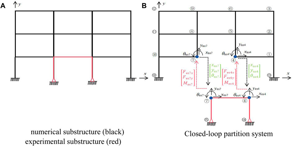
Figure 2. Substructure division and partition system. (A) Numerical substructure (black). (B) Closed-loop partition system experimental substructure (red).

Taking an example of a three-story experimental substructure, where the experimental substructure is the middle span of the first floor, and the rest is the numerical substructure, as shown in Figure 2A.

The numerical substructure and the experimental substructure are interconnected and synchronized through a feedback loop that allows them to share information at the common interface nodes at each time step during execution (Silva et al., 2020). Figure 2B shows the main degrees of freedom of the interface nodes and the signals transmitted between the numerical substructure and the experimental substructure. Ideally, at each time interval, the numerical substructure is first excited, then the responses ${\mathbf{\psi }}_{\text{ns}4}\left[4,16,28\right]={\left[x_{ns4}{y}_{ns4}{\theta }_{ns4}\right]}^T$ and ${\mathbf{\psi }}_{\text{ns}7}\left[7,19,31\right]={\left[x_{ns7}{y}_{ns7}{\theta }_{ns7}\right]}^T$ of the interface nodes are excited, their derivatives (velocity and acceleration) are added to the experimental substructure. Then, the generated experimental restoring forces ${\mathbf{f}}_{\text{es}4}={\left[F_{es4x}{F}_{es4y}{M}_{es4}\right]}^T$ and ${\mathbf{f}}_{\text{es}7}={\left[F_{es7x}{F}_{es7y}{M}_{es7}\right]}^T$ are measured and fed back to the numerical substructure. In addition, the more critical interface conditions in this paper are represented by vector ${\mathbf{\psi }}_{\text{ns}4}={\left[x_{\text{ns}4}{y}_{\text{ns}4}{\theta }_{\text{ns}4}\right]}^T,{\mathbf{\psi }}_{\text{ns}7}={\left[x_{\text{ns}7}{y}_{\text{ns}7}{\theta }_{\text{ns}7}\right]}^T,{\mathbf{\psi }}_{\text{es}4}={\left[x_{\text{es}4}{y}_{\text{es}4}{\theta }_{\text{es}4}\right]}^T,{\text{and}\mathbf{\psi }}_{\text{es}7}={\left[x_{\text{es}7}{y}_{\text{es}7}{\theta }_{\text{es}7}\right]}^T$.

The experimental substructure framework used in this paper is consists of a horizontal beam and two vertical columns. The beam element is made of a 50 mm × 6 mm plate (web) and two 38 mm × 6 mm plates (flanges), and the column elements are made of A572 Grade 50 structural steel. This experimental substructure framework has been used in the research of Gao and Castaneda (Gao, 2012; Gao et al., 2013b), and Silva (Silva et al., 2020) and others have used this framework to study the benchmark control problem, then the feasibility of this device has been verified.

3.2 Transmission system

Due to the strong non-linearity and MDOF characteristics of the experimental substructure, RTHS with multi-directional loading are required. In addition, due to the high axial stiffness of the columns, the axial deformation of the columns will be neglected, and the vertical degrees-of-freedom along the entire coordinate y direction is not considered. To represent the MDOF response of the experimental substructure in a more realistic way and the hydraulic actuators only provide motion, two hydraulic actuators will be used in the transmission system to equivalently replace the motion of the original frame node 4, as shown in Figure 3. Figure 3A shows that node 4 of the experimental substructure is mainly affected by the rotation and horizontal displacement of the numerical substructure, and Figure 3B shows that at least two hydraulic actuators are required to provide equivalent translational and rotational motion for node 4.

Figure 3

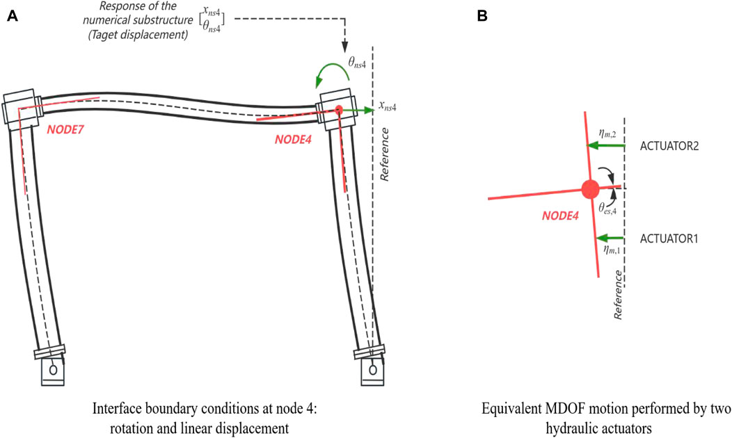
Figure 3. Equivalent multi-actuator action to provide both translational and rotational motion. (A) Interface boundary conditions at node 4: rotation and linear displacement. (B) Equivalent MDOF motion performed by two hydraulic actuators.

To better apply these two hydraulic actuators to the experimental substructure, this paper adds a coupler attached to the frame between the actuators and the frame, the specific hydraulic actuator and coupler settings refer to the literature cited in (JUC et al., 2023). The two hydraulic actuators directly act horizontally on the coupler, causing it to rotate and translate, thereby inducing equivalent MDOF motions in the frame, as shown in Figure 4.

Figure 4

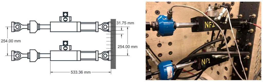
Figure 4. Both hydraulic actuators mounted on the wall (JUC et al., 2023).

3.3 MaRTHS scheme

With the numerical simulations model provided by the Benchmark Problem Platform (Silva et al., 2020), maRTHS is carried out, and its simulink diagram is shown in Figure 5. The main task of this scheme is to design a control system to make the measured actuator displacement consistent with the response of the numerical substructure in the actuator coordinates, and to evaluate its tracking performance and the overall performance of RTHS (Silva et al., 2020).

Figure 5

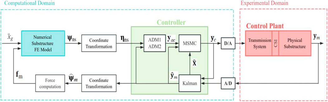
Figure 5. Simulink diagram of the ADM-MSMC method.

Figure 5 shows that the numerical substructure outputs a displacement vector ${\mathbf{\psi }}_{\text{ns}4}\left[4,28\right]={\left[x_{ns4}{\theta }_{ns4}\right]}^T$ under the action of ground motion. It is necessary to use a coordinate transformation function to convert this displacement vector from “frame coordinates ${\mathbf{\psi }}_{\text{ns}}$” to “actuator coordinates ${\mathbf{\eta }}_{\text{ns}}$,” and then input the transformed actuator coordinates into the control system to obtain the input vector ${\mathbf{y}}_c={\left[y_c^1{y}_c^2\right]}^{\mathrm{T}}$ for the control actuator. This signal is then transmitted to the corresponding hydraulic actuator, which drives the corresponding experimental substructure and obtains the multi-axis actuator displacement ${\mathbf{y}}_{\mathrm{m}}$ equivalent to the target displacement vector ${\mathbf{\psi }}_{\text{ns}}$ of the frame node. The multi-axis actuator displacement ${\mathbf{y}}_{\mathrm{m}}$ is then fed back to the control system. ${\widehat{\mathbf{\psi }}}_m$ is the vector of actuator responses transformed in frame coordinates. Similarly, this “actuator coordinate” is transformed by the coordinate transformation function into “frame coordinates,” and then the feedback force is calculated to obtain the experimental force vector ${\mathbf{f}}_{\mathrm{m}}$ required to satisfy the equilibrium condition at the interface nodes of the numerical substructure, and this feedback signal is fed back to the numerical substructure.

4 Numerical simulation

In this section, numerical simulations will be conducted using MATLAB/Simulink, with a primary focus on the time delay caused by actuators. In the simulation, the existing time delay compensation methods in the Benchmark Problem Platform are replaced with adaptive time series (ATS) (Chae et al., 2013), ADM, MSMC, and ADM-MSMC time delay compensation methods for RTHS. Experimental and numerical results are provided, followed by a comparison between the experimental and numerical results to validate the feasibility and robustness of the ADM-MSMC time delay compensation method.

In the Benchmark Problem Platform, the inherent actuator model is represented by transfer functions. In order to evaluate the robustness and stability of the proposed control methods, this paper defines partitioning situations by altering the structural parameters of the reference structure, as shown in Table 1. The variation of modal damping and mass for each layer of the reference structure is considered, resulting in different stability and performance scenarios. The input to the reference and hybrid system for this simulation is the EI Centro earthquake historic record with a scaling factor of 0.40. As shown in Figure 6, the inner-loop PI controller serves as the controller for the original Benchmark Problem Platform, which is in the transmission system as shown in Figure 5. The proportional gain (k_p) and integral gain (k_i) of the PI controller are set to k_p = 2 and k_i = 95, for detailed definitions, please refer to the literature cited in (Silva et al., 2020).

Table 1

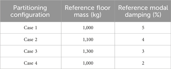
Table 1. RTHS partitioning cases.

Figure 6

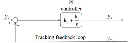
Figure 6. Block diagram of the control plant (Silva et al., 2020).

Where s is Laplace operator.

The parameters used herein for the these controllers are determined based on the parameters of the benchmark problem model, as summarized in Table 2 below. In this simulation, the solver was set to a fixed-step configuration with a base sample time of 1/1,024 s. The ODE4 (Runge-Kutta) method was chosen as the solver, providing a balanced approach between computational efficiency and accuracy for the simulation.

Table 2

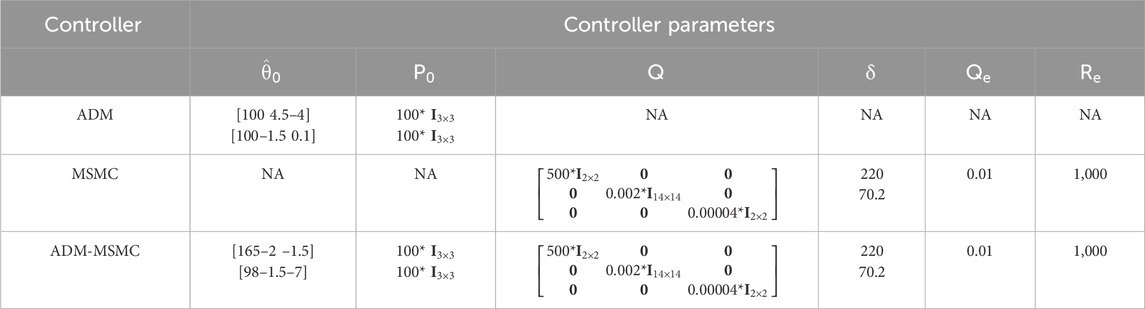
Table 2. Parameters of the controllers.

4.1 Displacement response

Due to space limitations, this paper only presents the displacement time-history comparison graphs for Case 1 and Case 4. Figures 7, 8 depict the displacement time-history curves for the different compensation methods in Case 1 and Case 4, respectively. The curves represent a comparison between the displacement time-history curves in the original Benchmark Problem Platform and the ones obtained by replacing the time-delay compensation method with ATS, ADM, MSMC, and ADM-MSMC methods. From Figures 7, 8, it is evident that replacing the original time delay compensation method in the Benchmark Problem Platform with the ADM-MSMC compensation method results in the actual displacement responses of actuator 1 and actuator 2 closely matching the desired displacement responses. Furthermore, compared to replacing with ATS, ADM, and MSMC methods, the actual displacement response curve of the ADM-MSMC method aligns more closely with the desired displacement response curve. This indicates that the proposed ADM-MSMC method exhibits higher compensation accuracy in maRTHS.

Figure 7

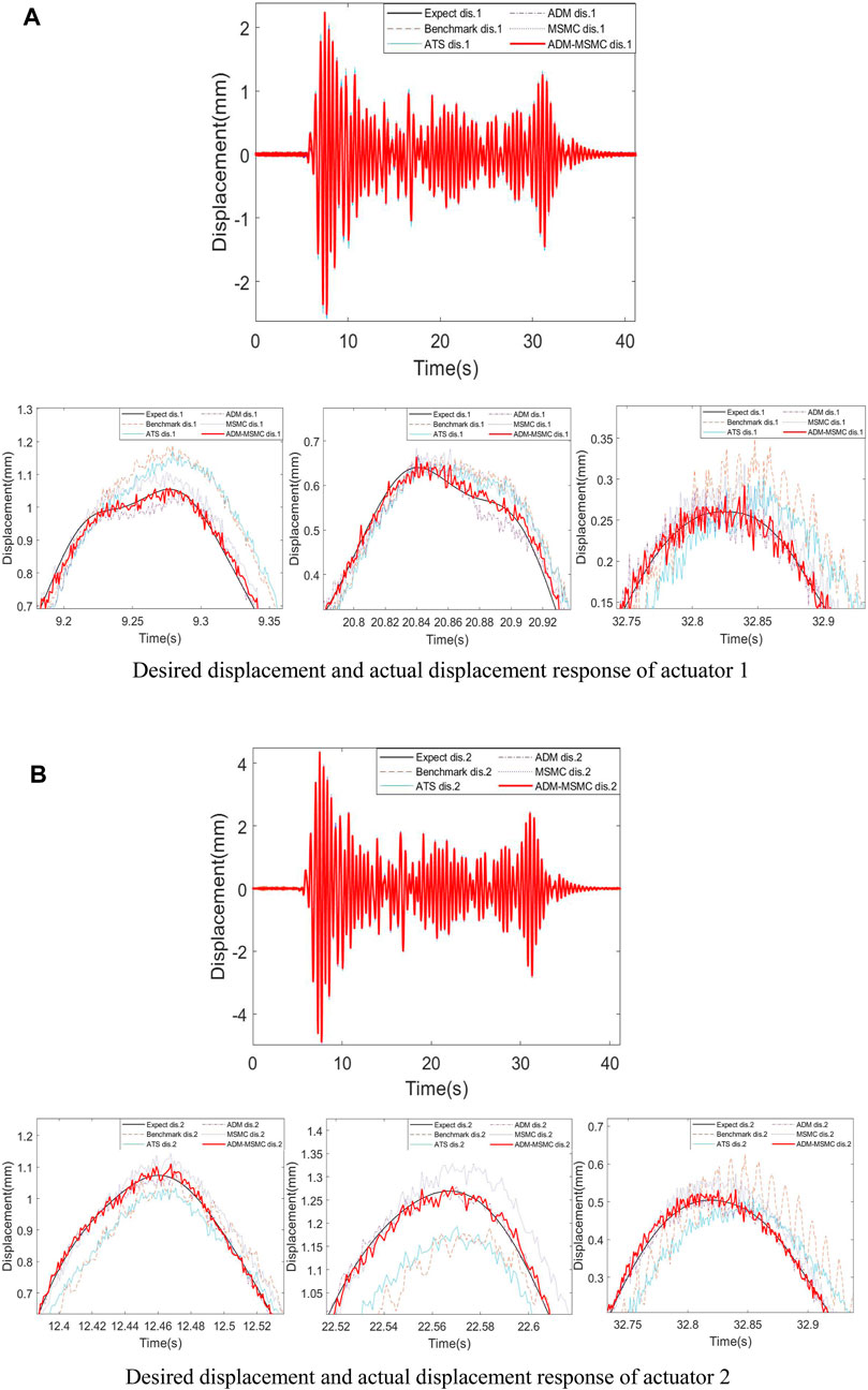
Figure 7. Displacement time-history comparison of Case 1. (A) Desired displacement and actual displacement response of actuator 1. (B) Desired displacement and actual displacement response of actuator 2.

Figure 8

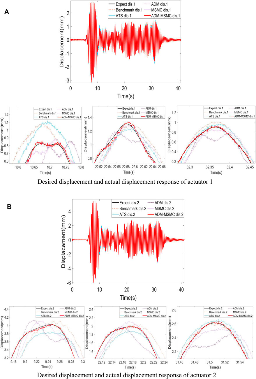
Figure 8. Displacement time-history comparison of Case 4. (A) Desired displacement and actual displacement response of actuator 1. (B) Desired displacement and actual displacement response of actuator 2.

4.2 Evaluation criteria values

To quantitatively assess the overall performance of maRTHS, this paper considers: 1) tracking control performance (minimization of error between target displacement and measured displacement); and 2) global RTHS experimental performance (minimization of error between reference structural response and hybrid system response). This simulation instance involves a set of 10 evaluation criteria, with the J₁ to J₆ assessing the tracking performance of the control system, and the J₇ to J₁₀ calculating the global performance of RTHS. The definitions and computation formulas of these criteria are detailed in reference (JUC et al., 2023).

The values of these ten evaluation criteria for four case are computed based on the numerical simulations responses, listed as A1-A4 in Supplementary Appendix SA, with the minimum value in each row bold for easier observation. This section presents line graphs of evaluation indicators analysis for four cases, as depicted in Figure 9, based on the four tables in Supplementary Appendix SA. In the graph, the horizontal axis ranging from 1 to 24 corresponds to performance indicators J_1,1 to J_10,27, with the specific numerical values of the performance indicators represented on the vertical axis. From Figure 9, it is evident that the values of J₁ to J₁₀ are relatively large without compensation, but show improvement after the application of compensation methods. Furthermore, it will be observed from Figure 9 that, except for the MSMC method and without compensation, other compensation methods exhibit smaller time delay between the desired and actual actuator displacements (J₁). Additionally, the ADM-MSMC method demonstrates relatively smaller normalized tracking error (J₂) and maximum peak tracking error (J₃) compared to other methods, indicating that the tracking performance of the ADM-MSMC method is more reliable than the other compensation methods considered in this paper. Moreover, the values of J₄ to J₁₀ for the ADM-MSMC method are smaller than those for the other four compensation methods. This suggests that the errors between the displacement responses of the ADM-MSMC method and the computed results of the reference model are also smaller, further validating the feasibility and robustness of the ADM-MSMC method.

Figure 9

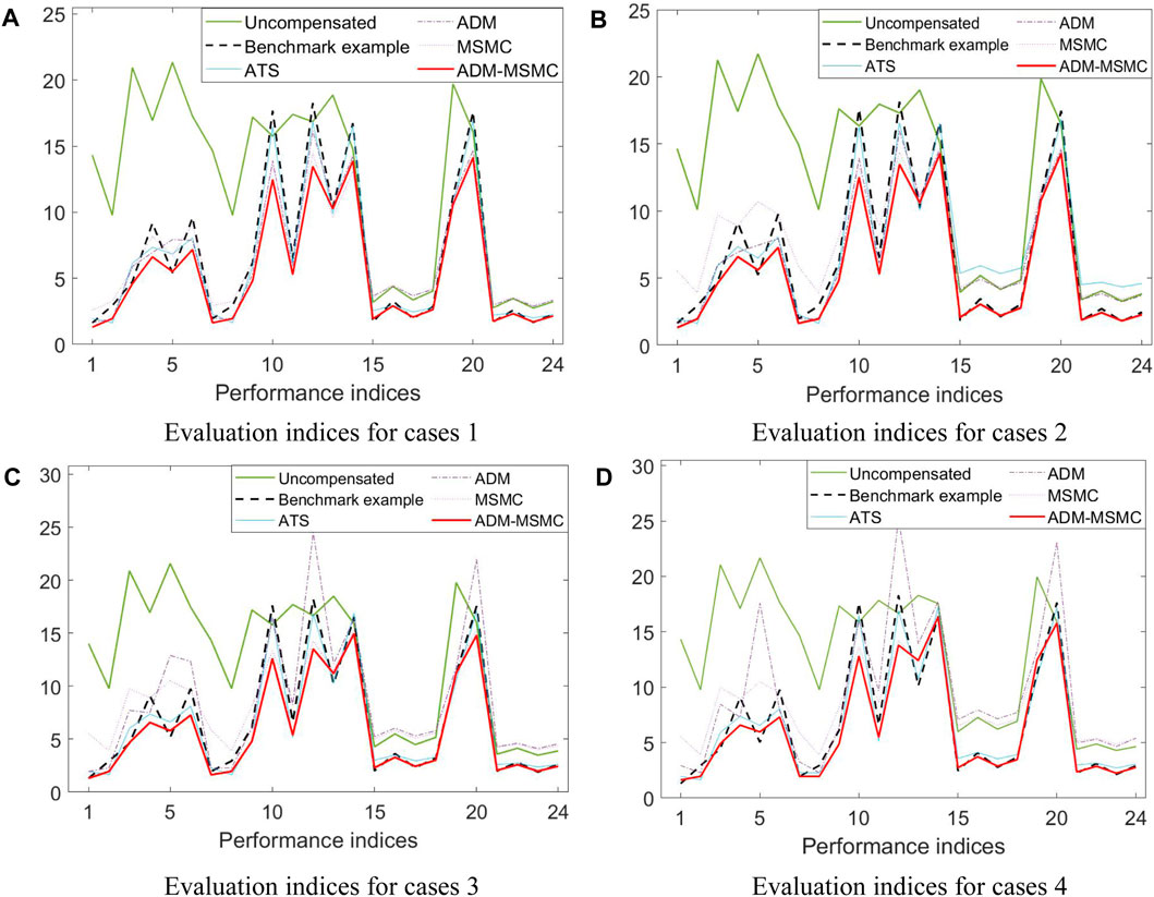
Figure 9. Evaluation indices for cases 1, 2, 3, and 4. (A) Evaluation indices for cases 1. (B) Evaluation indices for cases 2. (C) Evaluation indices for cases 3. (D) Evaluation indices for cases 4.

5 Conclusion

This paper proposes an ADM-MSMC method to compensate for the delay inherent in maRTHS, applied to the benchmark control problem of maRTHS. The principle and design of the ADM-MSMC method is introduced, with a focus on integrating ADM with MSMC. Numerical simulations of RTHS are conducted on the Benchmark Problem Platform, comparing the results of the ADM-MSMC compensated system with those of the original Benchmark Problem Platform, as well as those compensated using ATS, ADM, and MSMC methods. The numerical and simulation results demonstrate that when the ADM-MSMC method is applied to the maRTHS, the responses after ADM-MSMC compensation are more accurate and closely match the desired responses. Furthermore, the ADM-MSMC method exhibits greater feasibility and robustness compared to the other four compensation methods. Therefore, this method demonstrates a certain level of effectiveness in maRTHS.

Data availability statement

The datasets presented in this study can be found in online repositories. The names of the repository/repositories and accession number(s) can be found in the article/Supplementary Material.

Author contributions

YS: Software, Writing–original draft, Writing–review and editing. ZW: Methodology, Writing–review and editing. YG: Methodology, Software, Data curation, Investigation, Project administration, Resources, Writing–review and editing. YC: Software, Writing–review and editing. YZ: Software, Writing–review and editing. HZ: Writing–review and editing.

Funding

The author(s) declare that financial support was received for the research, authorship, and/or publication of this article. Thanks to the National Key Research and Development Program (2022YFC3801201), the National Natural Science Foundation of China (51878630, 52078398), and the Natural Science Foundation of Guangdong Province (2022A1515010500, 2022A1515010338).

Conflict of interest

The authors declare that the research was conducted in the absence of any commercial or financial relationships that could be construed as a potential conflict of interest.

Publisher’s note

All claims expressed in this article are solely those of the authors and do not necessarily represent those of their affiliated organizations, or those of the publisher, the editors and the reviewers. Any product that may be evaluated in this article, or claim that may be made by its manufacturer, is not guaranteed or endorsed by the publisher.

Supplementary material

The Supplementary Material for this article can be found online at: https://www.frontiersin.org/articles/10.3389/fbuil.2024.1393710/full#supplementary-material

References

Alejandro, P., and Mariantonieta, G. S. (2019). Adaptive tracking control for real-time hybrid simulation of structures subjected to seismic loading. Mech. Syst. Signal Process. 134 (12), 106345. doi:10.1016/j.ymssp.2019.106345

CrossRef Full Text | Google Scholar

Chae, Y., Kazemibidokhti, K., and Ricles, J. M. (2013). Adaptive time series compensator for delay compensation of servo-hydraulic actuator systems for real-time hybrid simulation. Earthq. Engng Struct. Dyn. 42 (11), 1697–1715. doi:10.1002/eqe.2294

CrossRef Full Text | Google Scholar

Chae, Y., Rabiee, R., Dursun, A., and Kim, C. Y. (2018). Real-time force control for servo-hydraulic actuator systems using adaptive time series compensator and compliance springs. Earthq. Engng Struct. Dyn. 47, 854–871. doi:10.1002/eqe.2994

CrossRef Full Text | Google Scholar

Chen, C., Ricles, J. M., and Guo, T. (2012). Improved adaptive inverse compensation technique for Real-Time Hybrid Simulation. J. Eng. Mech. 138 (12), 1432–1446. doi:10.1061/(asce)em.1943-7889.0000450

CrossRef Full Text | Google Scholar

Fermandois, G. A., and Spencer, B. F. (2017). Model-based framework for multi-axial real-time hybrid simulation testing. Earthq. Eng. Eng. Vib. 16 (4), 671–691. doi:10.1007/s11803-017-0407-8

CrossRef Full Text | Google Scholar

Gao, X. (2012). “Development of a robust framework for real-time hybrid simulation: from dynamical system,” in Motion control to experimental error verification. Purdue University ProQuest Dissertations Publishing, 3556206.

Google Scholar

Gao, X., Castaneda, N., and Dyke, J. S. (2013a). Experimental validation of a generalized procedure for mDOF real-time hybrid simulation. J. Eng. Mech. 140 (4), 04013006. doi:10.1061/(asce)em.1943-7889.0000696

CrossRef Full Text | Google Scholar

Gao, X., Castaneda, N., and Dyke, S. J. (2013b). Real time hybrid simulation: from dynamic system, motion control to experimental error. Earthg Eng. Struct. Dyn. 42, 815–832. doi:10.1002/eqe.2246

CrossRef Full Text | Google Scholar

Hayati, S., and Song, W. (2017). An optimal discrete-time feedforward compensator for real-time hybrid simulation. Smart Struct. Syst. 20 (4), 483–498. doi:10.12989/sss.2017.20.4.483

CrossRef Full Text | Google Scholar

Horiuchi, T., Inoue, M., Konno, T., and Namita, Y. (1999). Real-time hybrid experimental system with actuator delay compensation and its application to a piping system with energy absorber. Earthq. Engng Struct. Dyn. 28, 1121–1141. doi:10.1002/(sici)1096-9845(199910)28:10<1121::aid-eqe858>3.3.co;2-f

CrossRef Full Text | Google Scholar

Jiang, Z., Jian, Z. Q., Cheng, G., Ma, J., and Dong, S. M. (2020). Three-dimensional scene construction based on missile semi-physical simulation. Electron. Des. Eng. 28 (15), 83–87. doi:10.14022/j.issn1674-6236.2020.15.019

CrossRef Full Text | Google Scholar

Juc, W., Manuel, S., Edwin, P., Montoya, H., Dyke, S. J., Silva, C. E., et al. (2023). Experimental benchmark control problem for multi-axial real-time hybrid simulation. Front. Built Environ. 9. doi:10.3389/fbuil.2023.1270996

CrossRef Full Text | Google Scholar

Liu, Z. (2020). Real-time hybrid test method and hybrid simulation study of axle vibration system. Harbin Institute of Technology.

Google Scholar

Najafi, A., Fermandois, G. A., Dyke, S. J., and Spencer, B. F. (2023). Hybrid simulation with multiple actuators: a state-of-the-art review. Eng. Struct. 276, 115284. doi:10.1016/j.engstruct.2022.115284

CrossRef Full Text | Google Scholar

Najafi, A., and Spencer, B. F. (2021). Multiaxial real-time hybrid simulation for substructuring with multiple boundary Points. J. Struct. Eng. 147 (11). doi:10.1061/(asce)st.1943-541x.0003138

CrossRef Full Text | Google Scholar

Ning, X., Huang, N. W., Xu, G. S., Wang, Z., Wu, B., Zheng, L., et al. (2023). A novel model-based adaptive feedforward-feedback control method for real-time hybrid simulation considering additive error model. Struct. Control Health Monit. 2023, 1–25. doi:10.1155/2023/5550580

CrossRef Full Text | Google Scholar

Ou, G., Ozdagli, A. I., Dyke, S. J., and Wu, B. (2015). Robust integrated actuator control: experimental verification and real-time hybrid-simulation implementation. Earthq. Engng Struct. Dyn. 44 (3), 441–460. doi:10.1002/eqe.2479

CrossRef Full Text | Google Scholar

Ou, J. P. (2003). Structural vibration control - active, semi-active and intelligent control. Beijing: Science Publishing House, 71–74.

Google Scholar

Philips, B. M., and Spencer, B. F. (2011). Model-based feedforward-feedback tracking control for real-time hybrid simulation. NSEL Rep. Ser. doi:10.1061/(ASCE)ST.1943-541X.0000606

CrossRef Full Text | Google Scholar

Rajabi, N., Abolmasoumi, H. A., and Soleymani, M. (2018). Sliding mode trajectory tracking control of a ball-screw-driven shake table based on online state estimations using EKF/UKF. Struct. Control Health Monit. 25 (4), e2133. doi:10.1002/stc.2133

CrossRef Full Text | Google Scholar

Salvatore, S., and Mario, T. (2016). Actuator dynamics compensation for real-time hybrid simulation: an adaptive approach by means of a nonlinear estimator. Nonlinear Dyn. 85 (4), 2353–2368. doi:10.1007/s11071-016-2831-0

CrossRef Full Text | Google Scholar

Sarebanha, A., Schellenberg, H. A., Schoettler, J. M., Mosqueda, G., and A. Mahin, S. (2019). Real-time hybrid simulation of seismically isolated structures with full-scale bearings and large computational models. Comput. Model. Eng. Sci. 120 (3), 693–717. doi:10.32604/cmes.2019.04846

CrossRef Full Text | Google Scholar

Silva, C. E., Gomez, D., Maghareh, A., Dyke, S. J., and Spencer, B. F. (2020). Benchmark control problem for real-time hybrid simulation. Mech. Syst. Signal Process. 135, 106381. doi:10.1016/j.ymssp.2019.106381

CrossRef Full Text | Google Scholar

Stoten, D. P., Yamaguchi, T., and Yamashita, Y. (2016). Dynamically substructured system testing for railway vehicle pantographs. J. Phys. Conf. Ser. 744, 012204. doi:10.1088/1742-6596/744/1/012204

CrossRef Full Text | Google Scholar

Tian, Y. P., Wang, T., Zhou, H. M., and Du, C. (2022). Shaking-table substructure test using a MDOF boundary-coordinating device. Earthq. Eng. Struct. Dyn. 51 (15), 3658–3679. doi:10.1002/eqe.3741

CrossRef Full Text | Google Scholar

Wallace, M. I., Wagg, D. J., and Neild, S. A. (2005). An adaptive polynomial based forward prediction algorithm for multi-actuator real-time dynamic substructuring. Proc. R. Soc. A 461 (2064), 3807–3826. doi:10.1098/rspa.2005.1532

CrossRef Full Text | Google Scholar

Wang, Z., Ning, X., Xu, G., Zhou, H., and Wu, B. (2019). High performance compensation using an adaptive strategy for real-time hybrid simulation. Mech. Syst. Signal Process. 133, 106262. doi:10.1016/j.ymssp.2019.106262

CrossRef Full Text | Google Scholar

Wang, Z., Xu, G., Li, Q., and Wu, B. (2020). An adaptive delay compensation based on a discrete system model for real-time hybrid simulation. Smart Struct. Syst. 25 (5), 569–580. doi:10.12989/sss.2020.25.5.569

CrossRef Full Text | Google Scholar

Wu, B., Wang, Z., and Bursi, O. S. (2013). Actuator dynamics compensation based on upper bound delay for real-time hybrid simulation. Earthq. Engng Struct. Dyn. 42 (12), 1749–1765. doi:10.1002/eqe.2296

CrossRef Full Text | Google Scholar

Wu, B., and Zhou, H. (2014). Sliding mode for equivalent force control in real-time substructure testing. Struct. Control Health Monit. 21, 1284–1303. doi:10.1002/stc.1648

CrossRef Full Text | Google Scholar

Xu, D., Zhou, H., and Wang, T. S. (2019). Performance study of sliding mode controller with improved adaptive polynomial-based forward prediction. Mech. Syst. Signal Process. 133, 106263. doi:10.1016/j.ymssp.2019.106263

CrossRef Full Text | Google Scholar

Yang, B. Q., Ma, J., and Yao, Y. (2020). Progress and prospect of research on semi-physical simulation equipment for flight vehicles. Astronautical J. 41 (06), 657–665. doi:10.3873/j.issn.1000-1328.2020.06.003

CrossRef Full Text | Google Scholar

Yang, H. C., Tan, P., Yang, T. Y., and Zhou, F. L. (2021). Acceleration-based sliding mode hierarchical control algorithm for shake table tests. Earthq. Eng. Struct. Dyn. 50 (13), 3670–3691. doi:10.1002/eqe.3527

CrossRef Full Text | Google Scholar

Yang, H. C., Tan, P., Yang, T. Y., and Zhou, F. L. (2023). Shake table real-time hybrid testing for shear buildings based on sliding mode acceleration control method. Structures 52, 230–240. doi:10.1016/j.istruc.2023.03.140

CrossRef Full Text | Google Scholar

You, S., Gao, X., and Nelson, A. (2019). “Breaking the testing pyramid with virtual testing and hybrid simulation,” in Fatigue of aircraft structures, 1–10.

CrossRef Full Text | Google Scholar

Zhou, H., Wagg, D. J., and Li, M. (2017). Equivalent force control combined with adaptive polynomial-based forward prediction for real-time hybrid simulation. Struct. Control Health Monit. 24 (11), e2018. doi:10.1002/stc.2018

CrossRef Full Text | Google Scholar

Zhou, H., Xu, D., Shao, X., Ning, X., and Wang, T. (2019). A robust linear-quadratic-Gaussian controller for the real-time hybrid simulation on a benchmark problem. Mech. Eng. Signal Process. 133 (1), 106260. doi:10.1016/j.ymssp.2019.106260

CrossRef Full Text | Google Scholar