Fault Detection in Modular Offshore Platform Connections Using Extended Kalman Filter

Within the Space@Sea project, funded by the Horizon 2020 program, a concept for a floating island was developed. The main idea is to create space in the offshore environment, which can be used to harvest renewable energy, grow food or build a maritime transport and logistic hub. The island is designed as an assembly of platforms, which are connected by ropes and fenders. These connection elements are considered critical, as they have to carry extreme loads in the severe offshore environment. At the same time, any failure in the connecting elements might put the entire platform structure at risk. This paper presents a feasibility study for the fault detection in the connection elements using Extended Kalman filters. For various test cases, typical parameters of the connecting elements are estimated from motion data of the structure. Thus, the technique reveals changes in the connections. For various test cases, it is shown that fault detection is possible. Not only a failure of a single connecting rope but also multiple faults in the system can be detected.

1. Introduction

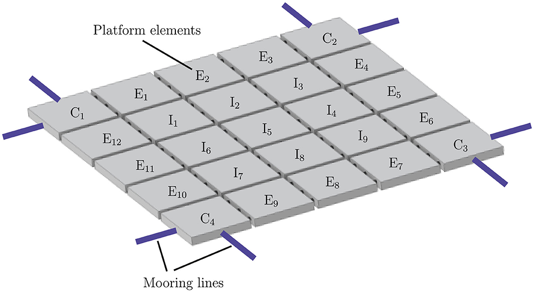
The Space@Sea project was launched in November 2017, as part of the EU innovation and research program Horizon 2020. The aim of this project was to develop a durable and sustainable solution for the creation of space in marine environments using flexible floating islands. For this purpose, a modular system consisting of floating multi-function platforms was developed. Initially, four use cases were defined: (1) A transport and logistics hub, (2) a facility for generating electricity from renewable sources, (3) a structure for aquaculture to produce food (Schultz-Zehden et al., 2018) and (4) a permanent habitat for people. The implementation of floating modular platforms as an additional terminal of a port is described in Souravlias et al. (2020). The easy implementation of a combination of several of these use cases was a key goal of the project and therefore, a major focus was put on the modularity of the platform system. Modularity was also a key factor for construction and maintenance of the system to allow for an easy connection and separation of individual elements (Flikkema and Waals, 2019). Figure 1 shows a possible platform arrangement of a setting with 25 platforms with mooring elements at the corner platform elements. The corner platforms are marked with “C,” the edge platforms with “E” and the platforms inside of the platform arrangement with “I.”

FIGURE 1

Figure 1. Platform arrangement of 25 connected platforms and eight mooring lines.

Environmental factors like wind and waves may cause significant forces on the platforms and in the connection elements. These forces essentially limit the number of possible locations, where it is safe to install such a platform structure. To keep the number of possible locations high, it is necessary to design the platform system for unshielded offshore areas. This means that the connection elements must be able to withstand very high forces. To guarantee the reliability of the platform arrangement and to decrease service costs, it is advantageous to detect potential faults in the platform connection elements as soon as possible. In this paper the pretensioned ropes, consisting of synthetic fibers, are assumed to be the critical elements of the system, as there are only three ropes and at least twelve fenders per side of a platform. Some advantages of synthetic fiber ropes are the lower weight, hence they are easier to install and need no grease, more detailed advantages are listed in Foster (2002). Decisions on the replacement of ropes are based upon visual inspections and the count of load cycles (Oland et al., 2017). Often visual inspection is only feasible by dismounting the ropes. Offshore rope surveying can be of high risk for investigators and require plenty of manpower. This is the case in the platform arrangement, where ropes run through pipes inside the modules, the rope dismantlement is dangerous and requires huge effort when carried out offshore.

The main damage mechanisms for fiber ropes are abrasion, creep, UV radiation, tensile fatigue, heating, compression fatigue, and shock (Oland et al., 2017). Rope fiber damages and fatigue affects the rope behavior like breaking strain, breaking stress, and stiffness change (Beltran and Williamson, 2011). The weakening of the platform connecting ropes lead to undesirable dynamic behavior of the platform arrangement. Higher strain of defect ropes leads to shocks and higher movement amplitudes of the platforms, which can be a reason that the platforms can no longer be used for the respective application. To avoid this effect, continuous rope condition monitoring is of major interest. Several condition monitor techniques for fiber ropes used in mooring offshore applications as vibrational techniques, magnetic resonance, conductive internal elements and fiber optics are shown in Beltran and Williamson (2011) and Gordelier et al. (2020). Some monitoring techniques require sensors inside the rope, therefore special rope design is necessary, which must not influence the rope structure. Another way is to determine physical rope values concluding rope faults. As the detailed platform design is in concept phase, indirect rope condition monitoring techniques are preferred. Therefore, the estimated rope stiffness was chosen as the relevant parameter for condition monitoring in this work.

There are studies which use fault detection techniques on offshore mooring lines. Hassani et al. (2018) uses dynamic hypothesis testing. Siréta and Zhang (2018) applies an artificial neural network in order to detect mooring line faults on offshore units based on GPS and motion sensors. Liu et al. (2020) shows mooring lines fault detection of floating offshore wind turbines using a wave-excited linear model based on Kalman filter algorithm for the JONSWAP spectrum. Kalman filter techniques can detect changes in parameters, which cannot be measured directly (Dan, 2006). The Kalman filter techniques has a wide range of applications. An overview about industrial applications of the Kalman filter can be found in Auger et al. (2013), applications of the Kalman filter for fault detection are shown in Eykeren et al. (2012), Jesussek and Ellermann (2014), and Ayaz (2015). Offshore applications of the extended Kalman filter to structural dynamic systems are shown in Imai et al. (1989) and Beltran and Williamson (2011), whereas hydrodynamic coefficients matrices with non-linear drag and linear inertia forces are identified for an offshore tower excited by wave forces. An important huge field of application of the Kalman filter technique in marine application is dynamic positioning. Most modern marine vessels use motion control systems to hold a certain position or to follow a desired path. Research in this area includes the implementation of the Kalman filter for ship motion and course keeping control systems, position and heading regulation, path following and trajectory tracking. A position and heading control system applying wave filtering using Kalman filters and Kalman filter design for ship course-keeping autopilots is shown in Perez (2010). The Application of the extended Kalman filter for moving horizon estimation for a marine dynamic positioning system is done by Zhao and Su (2015). In Triantafyllou et al. (1983), a Kalman filter is used for real time estimation of heave, pitch, roll, sway and yaw motion for a VTOL aircraft landing is shown. More applications of the Kalman filter for dynamic positioning can be found in Balchen et al. (1980), Grimble et al. (1980), and Alcocer et al. (2007).

As the platform arrangement shows a strongly non-linear behavior, non-linear parameter identification methods are considered. Many non-linear state observers were developed during the last decades, some applications are shown in Garrido et al. (2004), Lin and Betti (2004), Farza et al. (2009), and Torres et al. (2015). One observer which is able to estimate states and parameters of a non-linear dynamic system from indirect measurements is the extended Kalman filter, which is based on a standard Kalman filter observer used for linearized systems. Mu et al. (2017) overcomes instability problems of the extended Kalman filter due to real-time updating of the noise parameters. Koh et al. (1991) presents a substructure approach for the extended Kalman filter to estimate the stiffness and damping coefficients of a structure. This paper is a feasibility study to proof whether it is even possible to detect faults of dynamic systems with a huge amount of degrees of freedom by applying the extended Kalman filter algorithm. Therefore, these advanced Kalman filter techniques are not further considered. The Kalman filter provides estimates of unknown states and parameters in the presence of uncertainties. The non-linear multi-body system of the platform arrangement is known which is superimposed by some uncertainties, the system input is generated by time varying stochastic wave hight and the measurements is noisy. Concerning these circumstances, the extended Kalman filter observer is chosen for the rope stiffness estimation to detect faulty ropes based on acceleration data measured at different points of the platforms. With this method, faults in the rope connection elements, e.g., cracks or ruptured strands, can be detected as a change in the stiffness of the connection element. The presented paper demonstrates, on the basis of a simulated model, the possibility to estimate critical parameters using acceleration data.

2. Methodology

2.1. Multi-Body Platform System Dynamics

A multi-body system is a mechanical system that consists of coupled bodies, which undergo translational and rotational displacements under the influence of forces and moments. In multi-body models, the bodies have mass, but the connecting elements are considered massless. These coupling elements can either be force elements (e.g., springs or dampers) that connect two points of two bodies and exert a force or a moment on these bodies, or they can be binding elements (e.g., joints or guides) that define the position of one body relative to another. The focus of this analysis lies on the rigid body notations of the platform elements.

2.2. Concept of the Platform System

The proposed design concept for Space@Sea uses synthetic fiber ropes and elastomer fenders to connect the platform elements and keep them in safe distance of one another. A first conceptual test of a floating island, connected by ropes and fenders, consisting of triangular platforms, was done by Waals et al. (2018). Since the fields of applications for squared platforms are higher, squared platforms are considered in this work. In Figure 2 the arrangement of the synthetic fiber ropes, elastomer fenders and mooring lines on four platform elements placed on the corner of a platform array is shown. The platforms of the system differ by the number of adjacent platforms. There are interior platforms (I), with adjacent platforms on all sides, platforms placed on the corner of the system (C), with two adjacent platforms and edge platforms (E), with no adjacent platform on one side. Considering the platform array with 25 platforms in Figure 1, there are nine platforms inside the platform array, named interior platforms I₁-I₉, 12 edge platforms with three adjacent platforms E₁-E₁₂ and four corner platforms with two adjacent platforms C₁-C₄. The ropes are attached to the side area of the corner and edge platforms where there are no fenders. Acceleration sensors are situated on three different positions. The two diagonally opposite sensors measure the acceleration in x, y, and z direction, the third sensor measures the acceleration in z direction. Different configurations of ropes and fenders are possible. In this paper, we consider three fender elements between adjacent platform elements and three ropes per platform side. The twelve fenders per side, used at the Space@Sea project shown in Figure 2 are grouped to give three sets with four fenders.

FIGURE 2

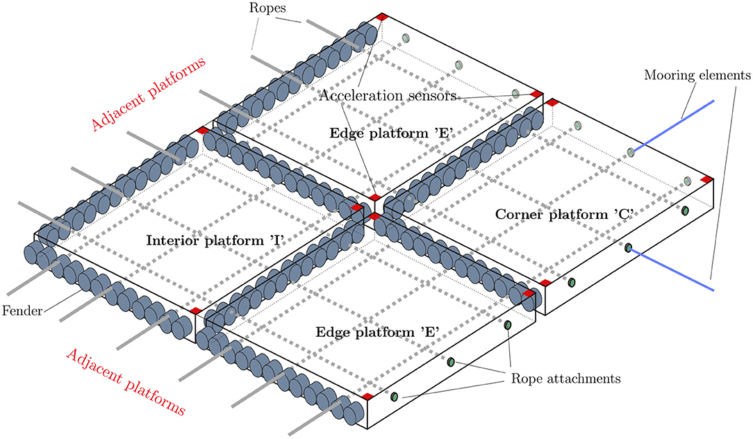
Figure 2. Arrangement of the synthetic fiber ropes, elastomer fenders, and mooring lines on four platform elements placed on the corner of a platform array with three acceleration sensors per platform.

The forces acting on the connection elements should be kept at acceptable levels even in severe sea states. The stiffness of the connection elements influences the forces significantly. As the stiffness of a rope decreases linearly with its length, it is necessary to use very long ropes, which go through the middle of the platform elements in watertight steel pipes and are connected on the exterior platform side area of the platform arrangement. In this paper, the very low friction between the pipe and the rope is neglected and the force in one rope is supposed to be constant along its length.

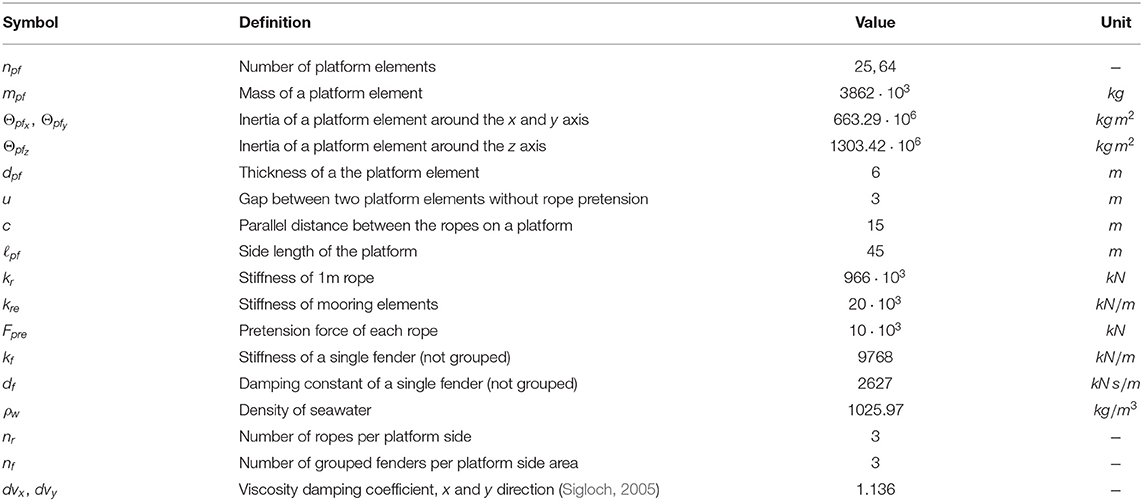
The ropes will be pre-stressed to assure system stability. Keeping tensile stress in the ropes at all times avoids heavy shock. On the other hand, sufficient pretension also avoids relative movement between the fender and the adjacent module. The amount of necessary pretension depends on the expected sea states at the platform location. The technical data of the platform and the necessary parameters for the multibody dynamic platform simulation are represented in Table 1.

TABLE 1

Table 1. Simulation settings.

To keep the whole platform system in place, mooring lines are connected at the side area of the corner platforms, as shown in Figures 1, 2. The mooring lines are linear springs in x and y direction, which are fixed at the center of gravity at the corner modules of the platform arrangement. They are not pretensioned and cannot transmit compressive forces.

The platform elements have six degrees of freedom, which results in 12 states. For the ith platform element of an arrangement this gives the state vector $x_{(i)}={[x\dot{x}y\dot{y}z\dot{z}{\phi }_x\stackrel{.}{{\phi }_x}{\phi }_y\stackrel{.}{{\phi }_y}{\phi }_z\stackrel{.}{{\phi }_z}]}_{(i)}^T.$ The state vector consists of the three position variables (x, y, z) and the three angles of orientation (φ_x, φ_y, φ_z) shown in Figure 3 and the corresponding translation and rotation velocities. For a complete platform arrangement of n_pf platforms the number of states is given by n_st = 12 n_pf.

FIGURE 3

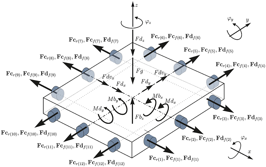
Figure 3. Forces and moments acting on a single platform element with adjacent platforms on all sides and three fender per side area.

The measurement states of the ith platform are defined as $y_{(i)}={[{\ddot{x}}_1{\ddot{y}}_1{\ddot{z}}_1{\ddot{x}}_2{\ddot{y}}_2{\ddot{z}}_2{\ddot{z}}_3]}_{(i)}^T$ with seven accelerations of three sensors measured in the platform coordinate system. For a platform array of n_pf platforms with sensors attached to all platforms there are n_meas = n_se n_pf measured accelerations, where n_se is the number of measured accelerations per platform.

2.2.1. The Newton-Euler Method

Various methods can be used to create solvable systems of equations for complex multi-body systems. The Newton-Euler method was chosen for the simulation of the Space@Sea platform system, because the forces in the connection elements, which are of main interest, appear explicitly in the equations and do not have to be calculated separately. The principles of linear and angular momentum conservation are used to create the differential equation system of the multi-body system. The difficulty of that procedure is, that a free body diagram of every body of the system is needed that is time-consuming for complex multi-body systems and therefore another method for creating the system of differential equations is mostly preferred to the Newton-Euler method (Woernle, 2011). The multi-body system examined in this paper is a modular system in which all elements are identical. Figure 3 shows a single platform, placed inside the platform array, with the forces and moments acting on it. Starting from this platform, the equations of motion are calculated from Equation (15), which is also applied for the edge- and corner platforms which only differ in having adjacent modules or not. If there is no adjacent platform to a side, shown in Figure 2 for an edge or a corner platform, fender forces of this side are set to zero. Also rope forces on this sides are not considered, hence rope forces inside the platform are internal force. At the corner platforms the mooring line forces are included. By applying the Newton-Euler method, only a single free body diagram and one set of differential equations is necessary to calculate the mechanical behavior of the platform system.

With the conservation of linear and angular momentum, six differential equations per module can be set up. In order to create a solvable system of differential equations, they must be set up in a common global coordinate system. Therefore, rotation matrices with cardan angles are used to rotate the relevant points (e.g., anchoring points of the connecting elements) from the respective local coordinate system into the global coordinate system. Cardan angles are characterized by sequencing the elementary rotations in order x-y-z. The elementary rotations are in relation to the already rotated axis. Multiplying the three rotation matrices of the elementary rotations results in the total rotation matrix A (Woernle, 2011):

$\begin{array}{ll}A=\left[\begin{array}{rrr}\hfill \cos {\phi }_y\cos {\phi }_z& \hfill -\cos {\phi }_y\sin {\phi }_z& \hfill \sin {\phi }_y\\ \hfill \cos {\phi }_x\sin {\phi }_z+\sin {\phi }_x\sin {\phi }_y\cos {\phi }_z& \hfill \cos {\phi }_x\cos {\phi }_z-\sin {\phi }_x\sin {\phi }_y\sin {\phi }_z& \hfill -\sin {\phi }_x\cos {\phi }_y\\ \hfill \sin {\phi }_x\sin {\phi }_z-\cos {\phi }_x\sin {\phi }_y\sin {\phi }_z& \hfill \sin {\phi }_x\cos {\phi }_z+\cos {\phi }_x\sin {\phi }_y\sin {\phi }_z& \hfill \cos {\phi }_x\cos {\phi }_y\end{array}\right]& (1)\end{array}$

By performing a left-sided multiplication of the matrix A with a position vector of any point on the platform, this point is transformed into the global coordinate system and can be used to set up the equations of linear and angular momentum conservation. In this paper, the points of interest are the anchoring points of the connecting elements fender and ropes, because with these global coordinates the length of the connecting elements are determined.

2.2.2. Forces and Moments Acting on the Platform

A single element, with the forces and moments acting on it, is depicted in Figure 3. Forces which are acting between the platform elements and the restraining of the corner elements to the environment, are generated by the ropes, mooring elements, and fenders. Under the assumption of linear elastic behavior, the spring forces in the connection elements can be calculated by

$\begin{array}{ll}F{c}_{(r,f,m)}=k\delta \ell r& (2)\end{array}$

where k is the spring stiffness of the connection element, δℓ is the difference of the current length compared to the length of the relaxed element and r is the vector of the direction of the acting force. The indices r, f, and m indicates whether a rope, fender, or mooring line force is calculated. It is supposed that the mooring elements do not change direction during simulation, they stay parallel to the x and y axis of the global coordinates. In this paper, the ropes and mooring elements can only transmit tensile forces and the fenders can only transmit pressure forces. If δℓ is positive at a fender connection or negative at a rope connection, the respective force is set to zero. For the fenders, linear damping is considered

$\begin{array}{ll}F{d}_f=d{v}_{rel},& (3)\end{array}$

where d = 4 d_f is the damping constant of the grouped fenders and v_rel is the relative velocity vector among the anchoring point of the fender and the associated point on the adjacent module. The associated point is the central support point of the fender on the adjacent module at the resting state of the system, where there are no external forces. Because of pretension and the resulting friction forces, this point will not change while the system is moving. The direction of the rope forces is determined from the direction vector, which connects the two anchoring points of the rope. The direction of the fender forces is determined with the direction vector, which connects the anchoring point of the fender and the associated point on the adjacent module.

Numerous external forces act on the multi-body system. However, not all of them have the same order of magnitude. In order to keep the complexity of the simulation low and therefore guarantee fast computing speed, only the dominant forces are considered. These are the buoyancy forces, gravitational force and forces that result from the flow resistance. The buoyancy force Fb_z of the ith platform element in z direction is defined by

$\begin{array}{ll}F{b}_{z_{(i)}}={\ell }_{pf}^{2}g{\rho }_w\left(w_{a{v}_{(i)}}+\frac{d_{pf}}{2}-z_{(i)}\right)& (4)\end{array}$

where g is the gravitational acceleration, w_av is the average wave hight based on the platform area, which is explained in more detail in section 2.2.3 and z is the z position of the respective platform. In addition to the buoyancy force in the z direction, the buoyancy moments Mb_x and Mb_y have to be calculated, which occur when the platform is rotating around the x or y axis. Therefore, the buoyancy is no longer symmetrical. The buoyancy moment Mb_x and Mb_y of the ith platform are calculated with

$\begin{array}{ll}M{b}_{x_{(i)}}=\text{−}\frac{1}{6}{\ell }_{pf}^4{\rho }_w\tan {\phi }_{x_{(i)}}\cos {\phi }_{x_{(i)}}g& (5)\end{array}$

$\begin{array}{ll}M{b}_{y_{(i)}}=\text{−}\frac{1}{6}{\ell }_{pf}^4{\rho }_{w}tan{\phi }_{y_{(i)}}cos{\phi }_{y_{(i)}}g& (6)\end{array}$

Here φ_x and φ_y are the angles of rotation of the platform around the x axis. The platform damping for the x, y, and z direction of the ith platform is calculated by

$\begin{array}{ll}F{d}_{x_{(i)}}=\text{−}{d}_x{ẋ}_{(i)}& (7)\end{array}$

$\begin{array}{ll}F{d}_{y_{(i)}}=\text{−}{d}_y{ẏ}_{(i)}& (8)\end{array}$

$\begin{array}{ll}F{d}_{z_{(i)}}=\text{−}{d}_z{ż}_{(i)}& (9)\end{array}$

and platform damping around the x and y axis by

$\begin{array}{ll}M{d}_{x_{(i)}}=\text{−}{d}_{\phi x}{\stackrel{\bullet }{\phi }}_{x_{(i)}}& (10)\end{array}$

$\begin{array}{ll}M{d}_{y_{(i)}}=\text{−}{d}_{\phi y}{\stackrel{\bullet }{\phi }}_{y_{(i)}}& (11)\end{array}$

where d_x, d_y, d_z, d_φx, and d_φy are the frequency dependent hydrodynamic damping coefficient and ẋ, ẏ, ż, ${\stackrel{\bullet }{\phi }}_x$, and ${\stackrel{\bullet }{\phi }}_y$ are the linear and angular components of the platform velocity. The effect of the surrounding fluid was accounted for as described in Newman (1977). This yields the damping terms d_x, d_y, d_z, d_φx, and d_φy used in Equations (7)–(11) and additional mass terms mx_add, my_add, mz_add, and additional inertia terms Θx_xadd, Θy_yadd used in Equation (15) (Supplementary Table 1). The effect of damping due to the rotation around the φ_z axis is neglected because of the small rotation speed around the z axis.

The drag in x and y direction of the ith platform, which is influenced by the viscosity of the water and is calculated by

$\begin{array}{ll}Fd{v}_{x_{(i)}}=\text{−}\frac{1}{2}d{v}_x{ẋ}_{(i)}^2{\rho }_w{\ell }_{pf}{t}_s& (12)\end{array}$

$\begin{array}{ll}Fd{v}_{y_{(i)}}=\text{−}\frac{1}{2}d{v}_y{ẏ}_{(i)}^2{\rho }_w{\ell }_{pf}{t}_s& (13)\end{array}$

where dv_x and dv_y are the drag coefficient in x and y direction, ẋ and ẏ are the platform velocities in x and y direction and t_s is the submersion depth of the platform. The weight force is calculated by

$\begin{array}{ll}{F}_g=\text{−}g{m}_{pf}.& (14)\end{array}$

The combination of the Equations (2)–(14) results in the equation of motion of the ith platform element describing the platform dynamics:

$\begin{array}{ll}{\left(\begin{array}{c}\ddot{x}\\ \ddot{y}\\ \ddot{z}\\ {\ddot{\phi }}_x\\ {\ddot{\phi }}_y\\ {\ddot{\phi }}_z\end{array}\right)}_{(i)}={\left(\begin{array}{c}\frac{1}{m_{pf}+m{x}_{add}}\left({\displaystyle {\sum }_{j=0}^{a{n}_r}F}{c}_{rx(j)}+F{c}_{mx}+{\displaystyle {\sum }_{j=0}^{a{n}_f}\left(F{c}_{fx(j)}+F{d}_{fx(j)}\right)}+Fd{v}_x+F{d}_x\right)\\ \frac{1}{m_{pf}+m{y}_{add}}\left({\displaystyle {\sum }_{j=0}^{a{n}_r}F}{c}_{ry(j)}+F{c}_{my}+{\displaystyle {\sum }_{j=0}^{a{n}_f}\left(F{c}_{fy(j)}+F{d}_{fy(j)}\right)}+Fd{v}_y+F{d}_y\right)\\ \frac{1}{m_{pf}+m{z}_{add}}\left({\displaystyle {\sum }_{j=0}^{a{n}_r}F}{c}_{rz(j)}+{\displaystyle {\sum }_{j=0}^{a{n}_f}\left(F{c}_{fz(j)}+F{d}_{fz(j)}\right)}+F{b}_z+F_g+F{d}_z\right)\\ \frac{1}{{\Theta }_{p{f}_x}+\Theta x_{xadd}}\left({\displaystyle {\sum }_{j=0}^{a{n}_r}M}{c}_{rx(j)}+{\displaystyle {\sum }_{j=0}^{a{n}_f}\left(M{c}_{fx(j)}+M{d}_{fx(j)}\right)}+M{d}_x+M{b}_x\right)\\ \frac{1}{{\Theta }_{p{f}_y}+\Theta y_{yadd}}\left({\displaystyle {\sum }_{j=0}^{a{n}_r}M}{c}_{ry(j)}+{\displaystyle {\sum }_{j=0}^{a{n}_f}\left(M{c}_{fy(j)}+M{d}_{fy(j)}\right)}+M{d}_y+M{b}_y\right)\\ \frac{1}{{\Theta }_{p{f}_z}}\left({\displaystyle {\sum }_{j=0}^{a{n}_r}M}{c}_{rz(j)}+{\displaystyle {\sum }_{j=0}^{a{n}_f}\left(M{c}_{fz(j)}+M{d}_{fz(j)}\right)}\right)\\ & \end{array}\right)}_{(i)}\hfill & (15)\end{array}$

The coefficient a in Equation (15) depends on the number of adjacent platforms of the ith platform in the platform array depicted in Figure 2. For interior platforms a = 4, for edge platforms a = 3 and for corner platforms a = 2. The mooring forces Fc_mx and Fc_my are included if there are mooring lines at the respective platform. The moments Mc_r(x,y,z), Mc_{f (x,y,z)}, and Md_{f (x,y,z)} are resulting from the forces Fc_r(x,y,z), Fc_{f (x,y,z)}, and Fd_{f (x,y,z)}, the moment acting from the mooring lines on the platform is neglected. For a platform array with n_pf platforms, the number of equations of motion is given by 6 n_pf. By solving these equations the states of the system are determined.

2.2.3. Ocean Wave Modeling

The main external forces exciting the structure are due to waves. Ocean wave characteristics depends on several factors, such as the wind speed, the distance over which the wind blows and the sea depth. There are different spectral descriptions of ocean waves (Pastor and Yucheng, 2016), e.g., by the Hubble proposed wave spectrum (Ochi and Hubble, 1976), the Pierson- Moskowitz (PM) (Pierson and Moskowitz, 1964) and the JONSWAP Spectrum (Hasselmann et al., 1973). In this paper, the ocean waves are modeled using the Pierson-Moskowitz power spectrum (Spanos, 1983). The PM power spectrum describes the energy distribution with frequency of wind generated fully developed ocean waves. For the simulation, a time series of the waves is generated by applying the autoregressive moving average (ARMA) algorithm to the PM power spectrum. The ARMA algorithm consists of the auto regressive (AR) and the moving average (MA) algorithm. The AR algorithm is ideal for treating all pole spectra and the MA algorithm is best suited for all zero spectra (Spanos, 1983). The PM spectra involves both poles and zeros, so the combination of the AR and MA overcomes this requirements and the ARMA algorithm is used in this paper. The AR part of the time series of the waves is defined as (Box et al., 1994) $w_k=u_k-\sum _{i=1}^p{a}_i{w}_{k-i}$ where u_k be the white noise, a₁, . . . , a_p are the AR parameters and w_k−1, . . . , w_k−p are the previous estimated AR wave hights. The sum of the a_i w_k−i can be shown as the weighted floated mean of the previous values w_k−1 where the AR-coefficients a are the weights. The MA component of the wave series is defined as $w_k=u_k+\sum _{j=1}^q{b}_j{u}_{k-j}$ where b₁, . . . b_q are the MA parameters which determine the weight of the white previous noise terms u_k−1, . . . , u_k−q. In matrix notation with the p × p matrix $A={\left[a,e_1,...,e_{p-1}\right]}^T$, where e_i is a p × 1 zero vector that is one in its i^th component and $a={(a_1,...,a_p)}^T$, the p × q matrix $B={\left[b,0_{q,p-1}\right]}^T$ with the q × 1 vector b = (b₁, …, b_q), the q × q matrix $V={\left[0_{q,1},e_1,\dots ,e_{q-1}\right]}^T$ and the auxiliary states v_k, the ARMA algorithm can be written as (Geist and Pietquin, 2011):

$\begin{array}{ll}\left(\begin{array}{c}{w}_k\\ v_k\end{array}\right)=\left[\begin{array}{cc}-A& B\\ 0_{q,p}& V\end{array}\right]\left(\begin{array}{c}{w}_{k-1}\\ v_{k-1}\end{array}\right)+\left(\begin{array}{c}{e}_1\\ e_1\end{array}\right)u_k& (16)\end{array}$

The ARMA coefficients now need to be chosen such that the process generates a spectrum according to PM with S(ω) is calculated according (Pierson and Moskowitz, 1964):

$\begin{array}{ll}S(\omega )=\frac{U}{{\omega }^5}exp\left(-\frac{V}{{\omega }^4}\right),& (17)\end{array}$

U = 8.2·10⁻³g² and $V=0.74{(g/v_{19.5})}^4$, where g represents the gravitation acceleration, ω the frequency of the spectrum and v_19.5 the wave producing wind speed measured 19.5 m above sea level. The determination of the coefficients in Equation (16) follows the work of Spanos (1983). It essentially results in a minimization

$\begin{array}{ll}{\displaystyle \sum _{n=0}^M}{\left[S({\omega }_n)-Ŝ({\omega }_n)\right]}^2\stackrel{!}{=}min,& (18)\end{array}$

where the coefficients of the ARMA algorithm are selected to give an approximated spectrum Ŝ(ω_n) close to the required spectrum (17). Figure 4 gives an example for such a spectral description. For the calculation of the buoyancy force in Equation (4), the average wave hight w_av, related to the platform base area, is considered.

FIGURE 4

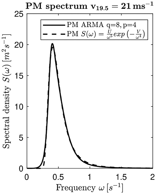
Figure 4. Comparison of the PM spectrum of a wind speed v_19.5 = 21m/s with the ARMA calculated PM spectrum.

The main task of the multi-body platform system described in section 2 is to generate acceleration data by the sensors. The following Kalman filter uses these acceleration data to estimate the states of the system, whereat the searched stiffness of the ropes are treated as states.

2.3. Fault Estimation of the Space@Sea Platform

After building the platform model and modeling the system input, the detection of faulty ropes is the main aim of this work. Changing stiffness parameters of the ropes are estimated by Kalman filters. These changing parameters, which can be an indication of a system fault, maybe difficult to measure directly in a mechanical system. In this section, the parameter estimation with the Kalman filter and the extended Kalman filter is explained, which is then used for the fault estimation of the Space@Sea platform array.

2.3.1. Basic Kalman Filter Equations

A deterministic continuous time linear system with its noise is described by a state equation and an output equations (Lunze, 2014):

$\begin{array}{ll}\stackrel{.}{x}=Ax+Bu+w& (19)\end{array}$

$\begin{array}{ll}\text{y}=C\text{x}+D\text{u}+\text{v}& (20)\end{array}$

where x is the state vector, y the output vector, $\stackrel{\bullet }{\text{x}}$ the derivation of x, u the system input, A the system-, B the input-, C the measurement, and D the feed-through matrix. The process noise w and the measurement noise v are both white noise with zero mean and uncorrelated. In this work, measurement and state values are discrete values, therefore the system is discretized with a sample time T. Furthermore, there is no feed-through matrix in the system. The discretized state space formulation of the linear system with the discretized system, input and measurement matrices F, G, and H is written in equations:

$\begin{array}{ll}{\text{x}}_k=F{\text{x}}_{k-1}+G{\text{u}}_{k-1}+{\text{w}}_{k-1}{\text{x}}_k\in {{R}}^{n_{st}\times 1}& (21)\end{array}$

$\begin{array}{ll}{\text{y}}_k=H{\text{x}}_{k-1}+{\text{v}}_k{\text{y}}_k\in {{R}}^{n_{meas}\times 1}& (22)\end{array}$

For optimal state estimation, the well-known Kalman filter is used (Kalman, 1960; Dan, 2006). After calculating the expected values of the initial state ${\widehat{\text{x}}}_0^{+}$ and $P_0^{+}$, the covariance of the initial state x₀, from Equations (23) and (24), the Kalman filter operates in two steps. In the prediction step, the measurement information at time step k is not known. The estimated state ${\widehat{\text{x}}}_k^{-}$, also named as a priori state (⁻), with all measurements information before, but not including time k is used, is calculated by the time update Equation (25). The time update of the covariance of the estimation error $P_k^{-}$ is calculated from Equation (26) where Q_k−1 is the disturbance input covariance matrix. In the correction steps the Kalman gain K_k, the estimated state ${\widehat{\text{x}}}_k^{+}$ and the covariance update matrix $P_k^{+}$ of the error covariance of ${\widehat{\text{x}}}_k^{+}$ are calculated in Equations (27)–(29). This includes the measurement information y_k up to and including time k. The estimated state ${\widehat{\text{x}}}_k^{+}$ is called the a posteriori (⁺) state. R_k is the measurement error covariance matrix.

The measurement covariance R_k and the process covariance matrix Q_k are known from the measurement noise v_k and process noise w_k, w_k ~ (0, Q_k), v_k ~ (0, R_k).

Initialization:

$\begin{array}{ll}{\widehat{\text{x}}}_0^{+}=E({\text{x}}_0)& (23)\end{array}$

$\begin{array}{ll}{P}_0^{+}=E[({\text{x}}_0-{\widehat{\text{x}}}_0^{+}){({\text{x}}_0-{\widehat{\text{x}}}_0^{+})}^T]& (24)\end{array}$

Prediction steps:

$\begin{array}{ll}{\widehat{\text{x}}}_k^{-}=F_{k-1}{\widehat{\text{x}}}_{k-1}^{+}+G_{k-1}{\text{u}}_{k-1}& (25)\end{array}$

$\begin{array}{ll}{P}_k^{-}=F_{k-1}{P}_{k-1}^{+}{F}_{k-1}^T+Q_{k-1}& (26)\end{array}$

Correction steps:

$\begin{array}{ll}{K}_k=P_k^{-}{H}_k^T{(H_k{P}_k^{-}{H}_k^T+R_k)}^{-1}& (27)\end{array}$

$\begin{array}{ll}{\widehat{\text{x}}}_k^{+}={\widehat{\text{x}}}_k^{-}+K_k({\text{y}}_k-H_k{\widehat{\text{x}}}_k^{-})& (28)\end{array}$

$\begin{array}{ll}{P}_k^{+}=(I-K_k{H}_k)P_k^{-}& (29)\end{array}$

2.3.2. Parameter Estimation and System Input Estimation

The Kalman filter cannot only be used for state estimation, also unknown system parameters can be estimated (Kopp and Orford, 1963; Dan, 2006). Periŝić et al. (2014) shows the application of the Kalman filter to estimate the structural loads of an offshore oil platform. Unknown system parameters are treated as additional components in the state vector. Faults in the ropes, connecting the platforms, can be found from changes in the stiffness values. To estimate these stiffness values, the state vector ${\text{x}}_k\in {{R}}^{n_{st}\times 1}$ is increased by additional components ${\text{x}}_p\in {{R}}^{n_p\times 1}$, to the extended state vector $x_e{}_k={[x_k^T,x_p^T]}^T,$ ${{R}}^{(n_{st}+n_p)\times 1}$. n_p is the number of parameters to estimate. For squared platform arrangements, e.g., 5 × 5, considered in this work, n_p is calculated by $n_p=2n_r\sqrt{n_{pf}}$.

2.3.3. The Extended Kalman Filter

The Kalman filter described in Equations (23)–(29) works for linear systems. To include the effect of non-linearities in our system, the extended Kalman filter is used in this work (Dan, 2006). Therefore, some approximations of the discretized non-linear system are necessary. The non-linear discretized system and measurement equations, including the extended states, are as follows:

$\begin{array}{ll}{\text{x}}_{{\text{e}}_k}=f_{k-1}({\text{x}}_{{\text{e}}_{k-1}},{\text{u}}_{k-1},{\text{w}}_{{\text{e}}_k})& (30)\end{array}$

$\begin{array}{ll}{\text{y}}_k=h_k({\text{x}}_{{\text{e}}_k},{\text{v}}_k)& (31)\end{array}$

Some non-linear Kalman filter techniques for state estimation of multi-body models can be found in Pastorino et al. (2012). To get a linear state transition matrix, the non-linear system is approximated by linearization about the operating point. Therefore, a Taylor series expansion, which is aborted after first term, is applied to the state equation (30) near ${\widehat{\text{x}}}_{{\text{e}}_{k-1}}^{+}$. The linearized state transition matrix is calculated from a partial derivative $A_{k-1}=\frac{\partial f_{k-1}}{\partial x_{e_k}}|{}_{x_{e_k}={\widehat{x}}_{e_{k-1}}^{+}}$ $\in {{R}}^{(n_{st}+n_p)\times (n_{st}+n_p)}$. The linearization of the output equation (31), near the operation point ${\widehat{\text{x}}}_{{\text{e}}_k}^{-}$, leads to the linearized output matrix $C_k=\frac{\partial h}{\partial x_e{}_k}{|}_{x_e{}_k={\widehat{x}}_{e_k}^{-}}$ $\in {{R}}^{(n_{meas})\times (n_{st}+n_p)}$. n_meas is the number of measured accelerations of the platform system. The process noise covariance matrix Q is calculated by $Q=B{\sigma }_{w_{av}}^2{B}^T$ $\in {{R}}^{(n_{st}+n_p)\times (n_{st}+n_p)}$, with ${\sigma }_{w_{av}}^2\in {{R}}^{(n_{pf})\times (n_{pf})}$ is the input noise covariance matrix of the average wave hights of each platform $w_{av}={[w_{av(1)},\dots ,w_{av(pf)}]}^T$ and B is the linearized input matrix calculated from a partial derivative $B=\frac{\partial f_0}{\partial w_{av}}{|}_{w_{av}=0}$ $\in {{R}}^{(n_{st}+n_p)\times n_{pf}}$ near the average wave hight of zero and the platform in equilibrium at the simulation start. The matrices A_k−1 and C_k are calculated at each time step k.

After calculating the expected values of the initial state ${\widehat{\text{x}}}_{{\text{e}}_0}^{+}$ and $P_{e_0}^{+}$, the covariance of the initial state x_e0, by Equations (23) and (24), the Kalman filter equations for the linearized system are calculated by:

$\begin{array}{ll}{\widehat{\text{x}}}_{{\text{e}}_k}^{-}=f_{k-1}({\text{x}}_{{\text{e}}_{k-1}}^{+},{\text{u}}_{k-1})& (32)\end{array}$

$\begin{array}{ll}{P}_{e_k}^{-}=A_{k-1}{P}_{e_{k-1}}^{+}{A}_{k-1}^T+Q& (33)\end{array}$

$\begin{array}{ll}{K}_k=P_{e_k}^{-}{C}_k^T{(C_k{P}_{e_k}^{-}{C}_k^T+R_k)}^{-1}& (34)\end{array}$

$\begin{array}{ll}{\widehat{\text{x}}}_{{\text{e}}_k}^{+}={\widehat{\text{x}}}_{{\text{e}}_k}^{-}+K_k\left({\text{y}}_k-h_k({\widehat{\text{x}}}_{{\text{e}}_k}^{-})\right)& (35)\end{array}$

$\begin{array}{ll}{P}_{e_k}^{+}=(I-K_k{C}_k)P_{e_k}^{-}& (36)\end{array}$

The covariance matrix of the initial estimate is

$\begin{array}{ll}{P}_{e_0}^{+}=\left[\begin{array}{cc}{P}_{x_{st}0}^{+}& 0\\ 0& P_{x_{p}0}^{+}\\ \end{array}\right]\in {{R}}^{(n_{st}+n_p)\times (n_{st}+n_p)},& (37)\end{array}$

where $P_{x_{st}0}^{+}$ and $P_{x_{p}0}^{+}$ are the matrices of the initial state covariance and the initial rope stiffness covariance. The covariance of the measurement noise is defined as

$\begin{array}{ll}{R}_k=\left[\begin{array}{ccc}{\sigma }_v^2& 0& 0\\ 0& \ddots & 0\\ 0& 0& {\sigma }_v^2\end{array}\right]\in {{R}}^{(n_{meas})\times (n_{meas})},& (38)\end{array}$

where ${\sigma }_v^2$ is the variance of the measurement noise. It is assumed, that the estimates of the initial states and the measurement noise are uncorrelated, there are only entries in the diagonal of $P_{e_0}^{+}$ and R_k.

The diagonal entries of the initial covariance of the estimated error $P_{x_{st}0}^{+}$ in 37 are set to 10⁻⁶ and 5·10⁻⁶ for $P_{x_{p}0}^{+}$. The variance of the measurement noise ${\sigma }_v^2$ in 38 is 4·10⁻⁴.

3. Results and Discussion

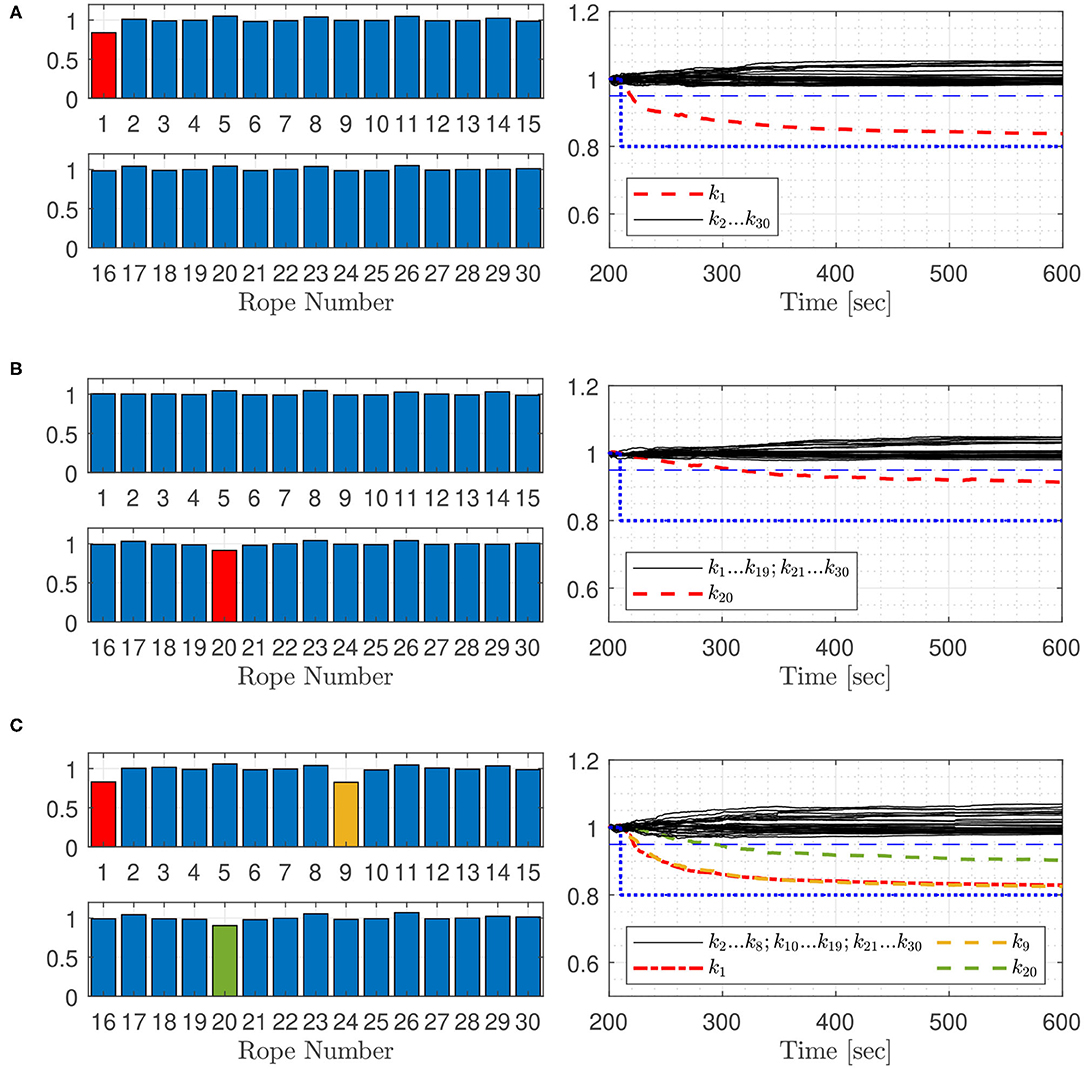
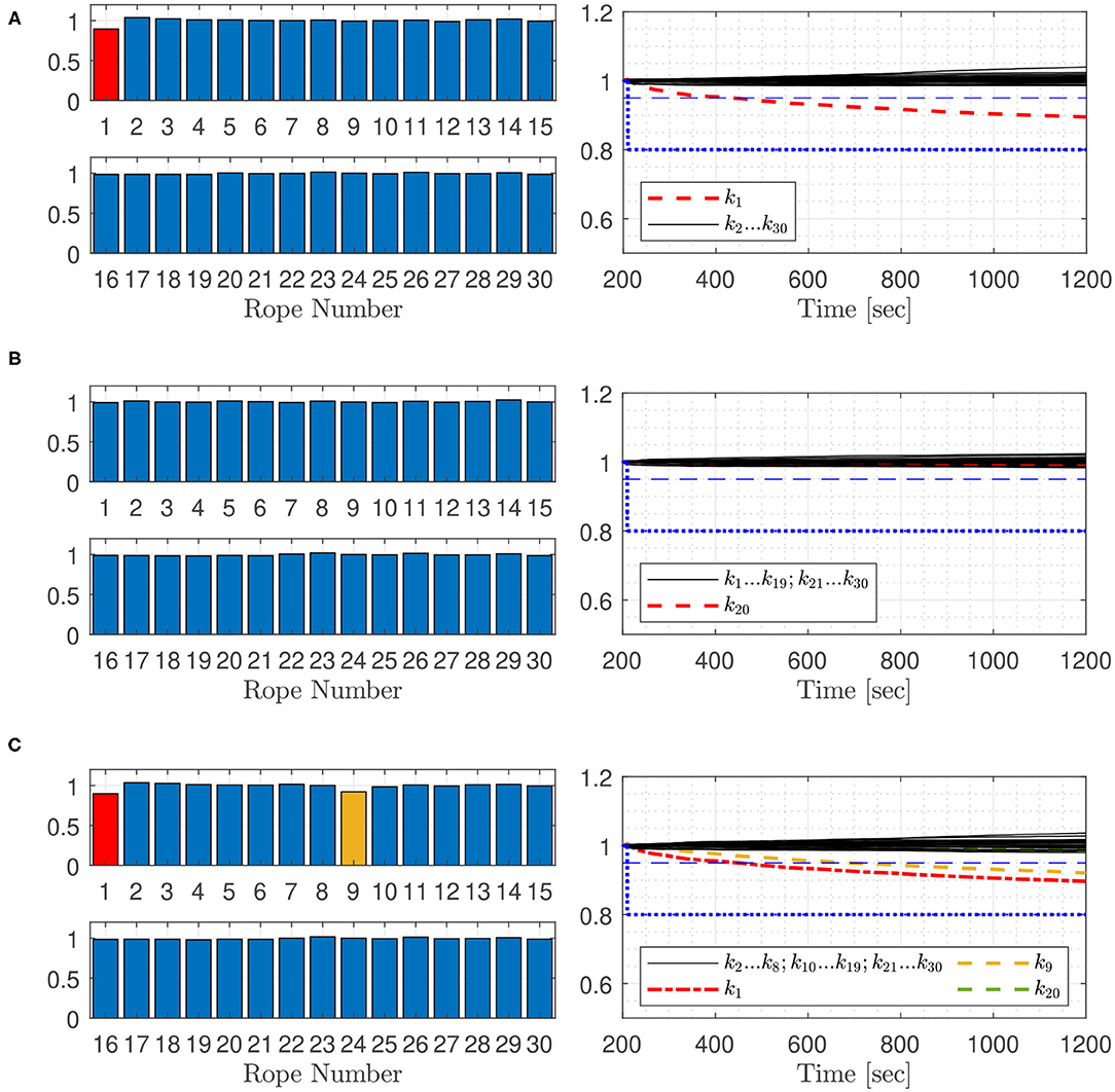
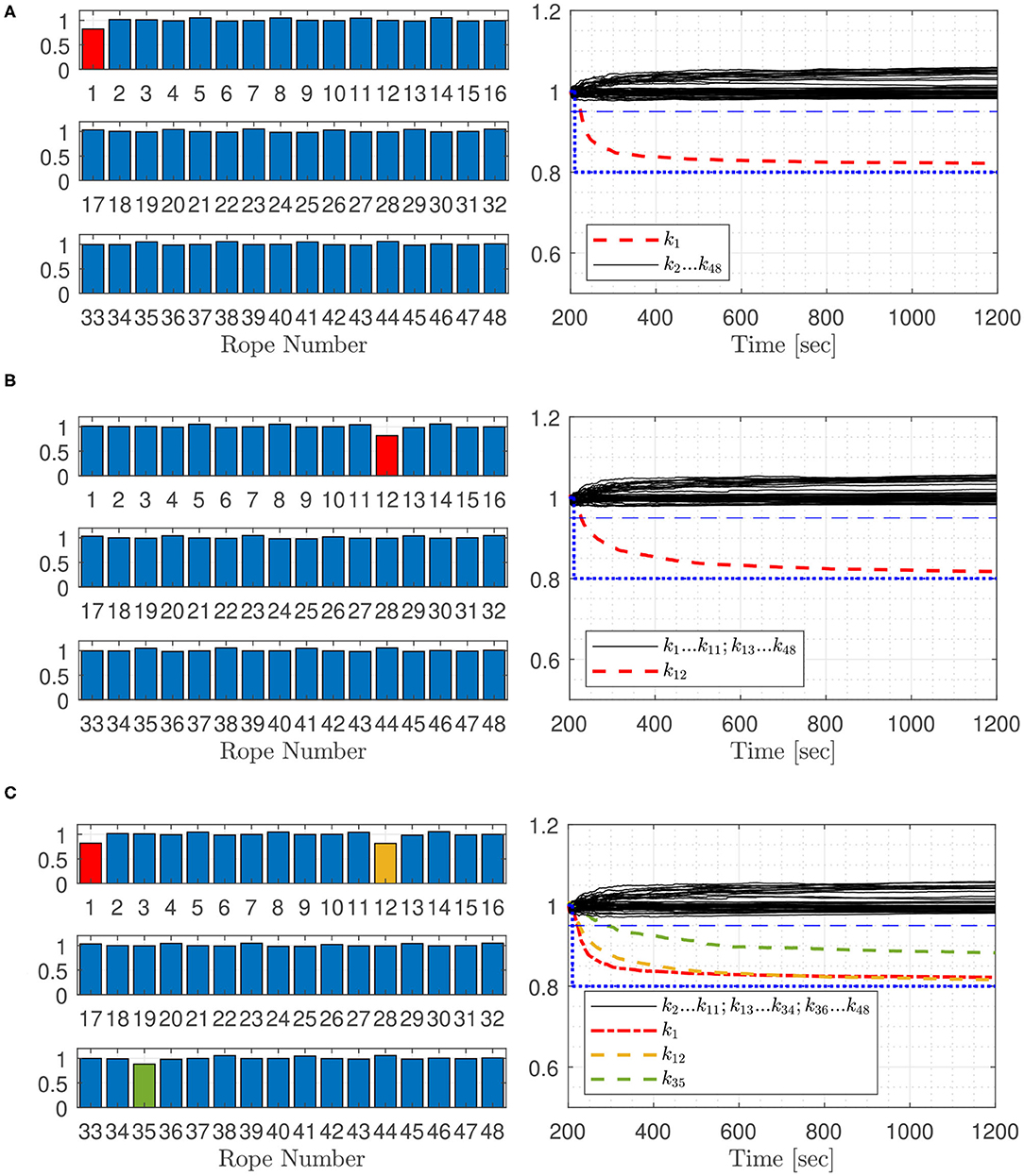
Parameter estimation using the Extended Kalman filter, is applied to detect faulty ropes of the Space@Sea platform arrangement. Parameters for the simulation model are summarized in Table 1. The platforms are excited by wind generated ocean waves, which are modeled by the Pierson- Moskowitz power spectrum. The model is used to generate data from the acceleration sensors, which are used in the estimation process. Different settings are reviewed: (a) one or more faults in selected ropes are assumed, (b) the wind speed is altered, (c) the platform array size is changed, and (d) the number of measured accelerations is varied. Simulation settings used in this work are shown in Table 2. The test case notation refers to the following diagrams, in this work squared platform arrays are considered. The ropes are numbered according Figure 5, represented for a squared 5 ×5 platform array with 25 platforms and 30 ropes. The simulation is starting when the platform elements are in equilibrium, not moving and the mooring elements are without tension. The measurement values are superimposed with a white noise with a variance of 0.0004 to include sensor noise. To decrease simulation effort, every 4th measurement value, which equates a time step of 0.2 s, is used for the iterative estimation process. For all simulations, after a simulation time of 210 s, the rope stiffness of faulty ropes in the model is set to 80% of the non-faulty rope which is indicated in Figures 7–12 by blue dotted lines. The Kalman filter fault detection process is launched 200 s after the simulation start. For better comparability of the estimated rope stiffness, the stiffness parameter is set to one for the non-faulty rope and 0.8 for the faulty ropes. A rope fault is indicated, when the normalized estimated rope stiffness is falling below the boundary of 0.95, which is indicated by a horizontal dashed line. The normalized estimated rope stiffness in the bar plots indicates the normalized estimated rope stiffness after 600 s in test case 1A, 1B, 1C, 2A, 2B, and 2C. For the other test cases, the normalized estimated rope stiffness is shown after 1,200 s. On the basis of the Figures 6–12, the trend of the estimated rope stiffness is explained for simulations carried out once. After this section, a higher number of simulations are included for selected test cases to test the repeatability of the simulations. Figure 13 shows statistical results of the rope fault detection time.

TABLE 2

Table 2. Test cases for the simulation.

FIGURE 5

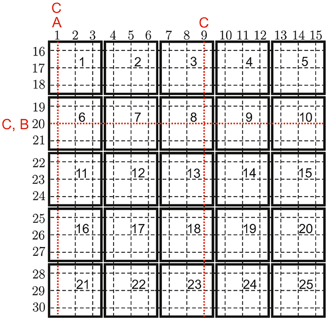
Figure 5. Rope numbering for a squared 5 × 5 platform array with 25 platforms and 30 ropes. Faulty ropes for test cases A, B, and C are marked.

FIGURE 6

Figure 6. Normalized estimated rope stiffness test case I, fault free system.

FIGURE 7

Figure 7. Normalized estimated rope stiffness test cases 1A (A), 1B (B), and 1C (C).

FIGURE 8

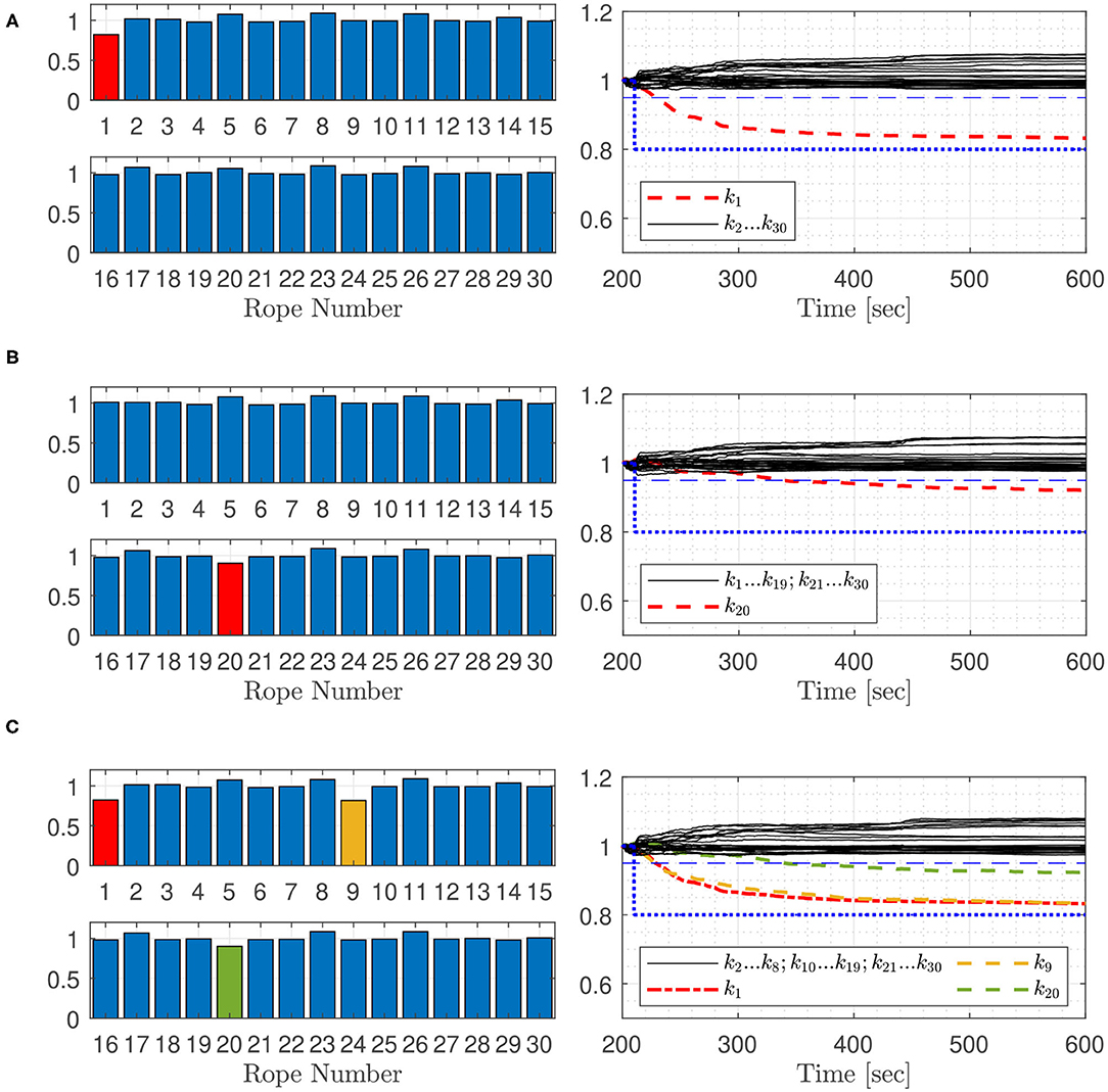
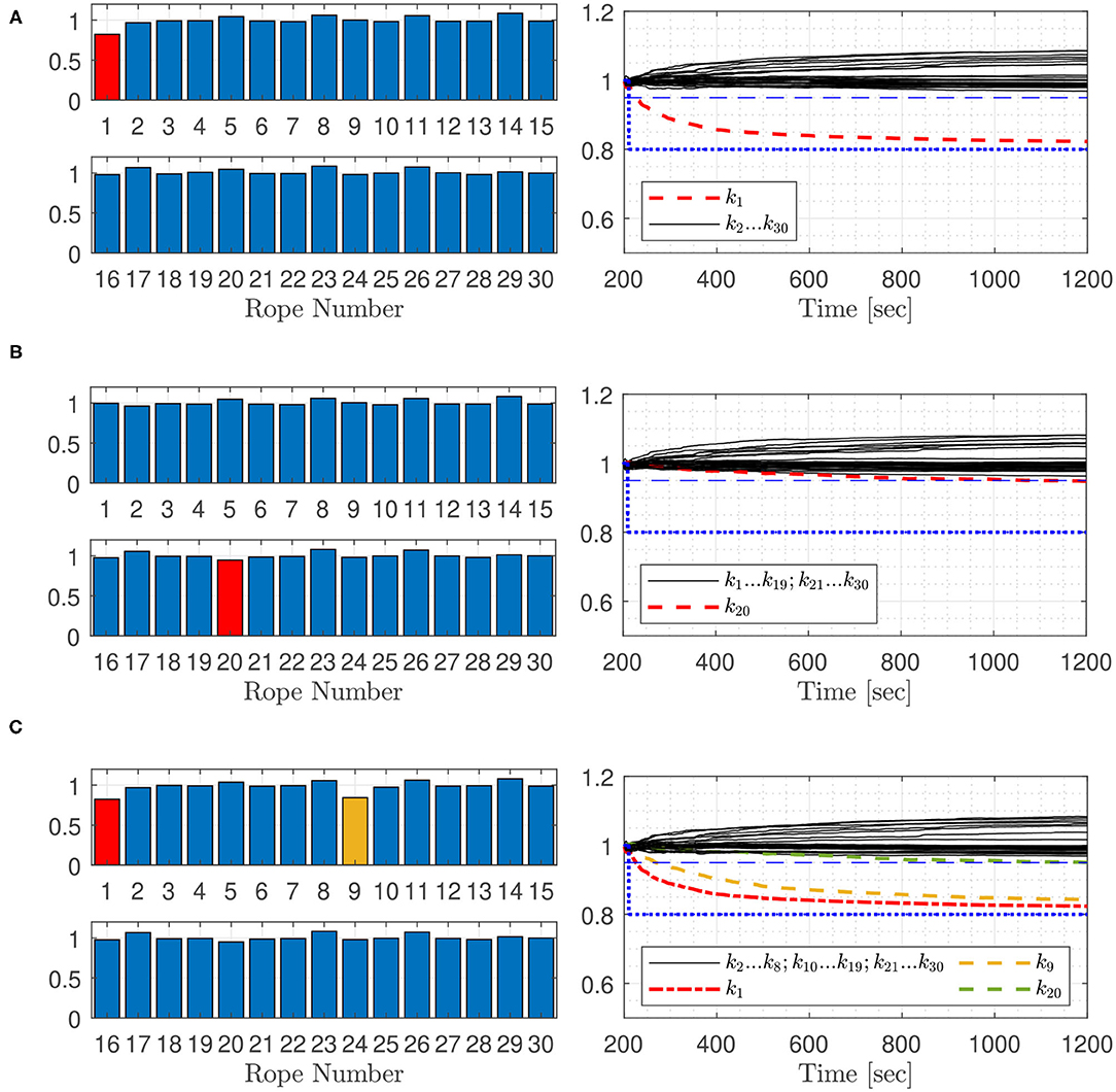
Figure 8. Normalized estimated rope stiffness test cases 2A (A), 2B (B), and 2C (C) including uncertainties of model parameters.

FIGURE 9

Figure 9. Normalized estimated rope stiffness test cases 3A (A), 3B (B), and 3C (C).

FIGURE 10

Figure 10. Normalized estimated rope stiffness test cases 4A (A), 4B (B), and 4C (C).

FIGURE 11

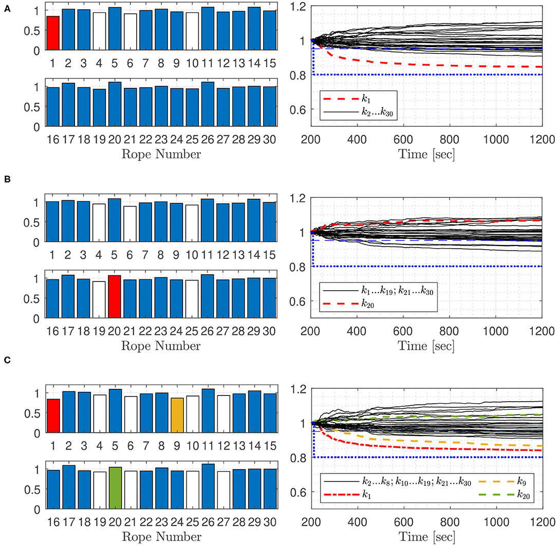
Figure 11. Normalized estimated rope stiffness test cases 5A (A), 5B (B), and 5C (C) with acceleration sensor only placed on the edge- and corner platforms.

FIGURE 12

Figure 12. Normalized estimated rope stiffness test cases 6A (A), 6B (B), and 6C (C).

FIGURE 13

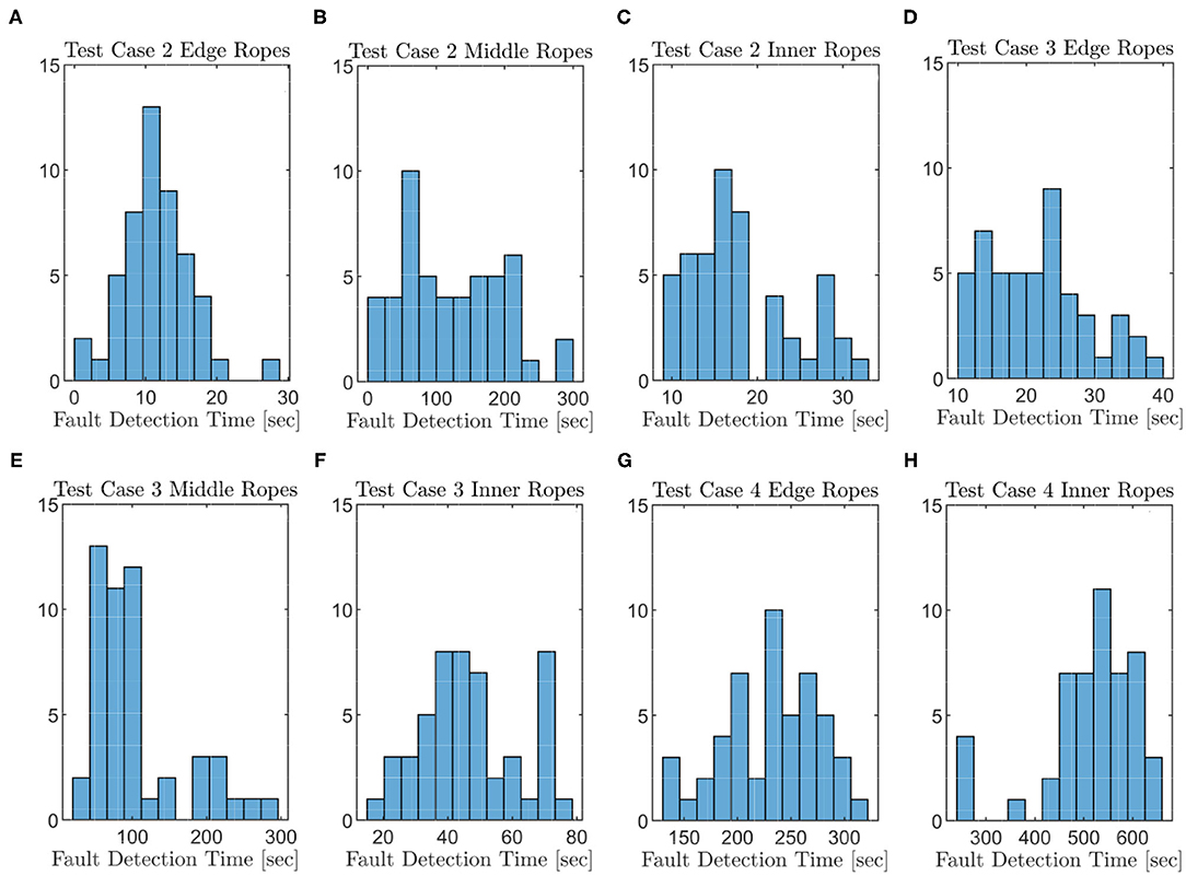
Figure 13. Fault detection time of test case 2 edge ropes (A), test case 2 middle ropes (B), test case 2 inner ropes (C), test case 3 edge ropes (D), test case 3 middle ropes (E), test case 3 inner ropes (F), test case 4 edge ropes (G), and test case 4 inner ropes (H).

Figure 6 gives the results for the fault free test case I, it can be seen that all estimated rope stiffness are near one, which indicates that there are no faults in the system.

Figure 7 shows test cases 1A, 1B, and 1C, where specific ropes are considered to have a significantly lower stiffness: In Figure 7A rope 1, in Figure 7B rope 20, and in Figure 7C ropes 1, 9, and 20 are considered to be faulty. The time until the fault is detected differs: Fault in rope 1 is estimated after 9 s, and fault in rope 20 after 101 s. All three faults in Figure 7C are estimated within 84 s.

In order to test the robustness of the filter against platform mass changes caused by different loading, against the deviation of fender properties and against different wave conditions, some parameters of the model are varied. The platform mass m_pf, the vertical damping value d_z, the additional mass in z direction mz_add, the fender damping d_f and the fender stiffness k_f are altered for all platforms by random values for the following simulations. All platform masses were altered by random values of ±1%, all vertical damping values by random values of ±5%, all additional masses in z direction by random values of ±5% and all fender stiffness and fender damping values by random values of ±10%. Figure 8 shows test cases 2A, 2B, and 2C with the same fault cases as Figure 7, including parameter variation for robustness examination. The results show, that all faults are detected. The uncertainties in the parameters leads to a longer detection time. The fault in rope 1, Figure 8A, is detected after 18 s, fault in rope 20, Figure 8B, after 126 s and all tree faults, Figure 8C, are estimated within 130 s after the faults set in. Stiffness in rope 20 is detected significantly later. Rope 20 is located between the ropes 19 and 21 as shown in Figure 5, which go through the same platforms. Changes in its stiffness are more difficult to detect. In this case the estimator has to distinguish between the cases of one fault in the middle rope, or two smaller faults in the parallel adjacent ropes. The effect of these cases on the overall dynamics of the system is relatively similar.

Figure 9 shows test cases 3A, 3B, and 3C for fault detection at a wind speed v_19.5 of 16 m/s. A fault in rope 1 is found after 16 s Figure 9A, a fault in rope 20 after 858 s with a narrow difference to other estimated rope stiffness Figure 9B. Three faults occur as depicted in Figure 9C, a fault in rope 20 is not indicated. Figure 9C shows that at a lower wind speed, a fault in rope 1 is estimated more than three times faster than a fault in rope 9. A change of stiffness in one of the ropes on the edge of the platform array, like ropes 1, 15, 16, or 30, has a higher influence on the platform dynamics than a stiffness change in ropes located inside the platform structure. Therefore, it is easier for the filter process to detect these rope faults. A changing stiffness of ropes inside the platform array with two adjacent parallel ropes is not as critical for the platform safety, because there are at least two parallel ropes nearby supporting the faulty rope, which is not the case for ropes placed on the edge of the platform array.

Figure 10 shows test cases 4A, 4B, and 4C for fault detection at a wind speed v_19.5 of 10 m/s. A fault in rope 1, Figure 10A and 1 and 9, Figure 10C can be detected, faults in rope number 20 were not detected, Figure 10B. The fault detection process needs more calculation steps as for the higher wind speed shown before. This is due to the low platform excitation, which results in small acceleration amplitudes measured by the sensors. Thus, the smaller values deliver less information for the estimating process.

Figure 11 shows the results for test cases 5A, 5B, and 5C, where the tree acceleration sensors per platform are just attached to the edge- and corner platforms, which reduces the number of acceleration sensors by 27. Test case 5A shows that the filter detects not only the faulty rope as defect, when the stiffness boundary of 95% is considered. There is a major difference between the estimated value of the faulty rope 1 and the false positive ropes 4, 6, and 10. Faults in rope 20, Figure 11B were not detected. Figure 11C shows the test case 5C with three faulty ropes. Faults in rope 20 were not detected. The estimated stiffness of the faulty ropes 1 and 9 have the lowest values. The difference to the false positive in rope 4, 6, 10, 12, 19, 21, 25, and 27 is small. Therefore, fault detection becomes unreliable, when only a small number of sensors is used in the analysis.

Figure 12 shows the results for test cases 6A, 6B, and 6C with a squared platform array of 64 platforms (Supplementary Figure 1) and acceleration sensors attached to all platforms. Forty-eight ropes are connecting the platforms, therefore the Kalman filter has to estimate 48 rope stiffness. Test case 6A in Figure 12A shows that the filter detects faults in rope 1, which is placed on the edge of the platform array, within 13 s. The faulty rope 12 in test case 6B is detected after 17 s (Figure 12B). The test case 6C with faults in rope 1, 12, and 35 shows that all faults are estimated within 79 s after the faults occurred (Figure 12C). Faults in rope 35 are detected significantly later. This rope goes through the center of its connecting platforms, and, again, has neighboring ropes to the left and right, which have a similar effect on the overall dynamics of the structure, making changes more difficult to detect.

The trend of the normalized estimated stiffness in Figures 7–12 differs by the location of the faulty ropes. The normalized estimated rope stiffness of ropes that go through the center of its connecting platforms, differ significantly compared to the normalized stiffness of the model after a simulation time of 600, respectively 1,200 s. These rope faults are more difficult to detect. The normalized estimated rope stiffness of the residual faulty ropes nearly reach the normalized stiffness value of the faulty rope of the model if the wind speed is hight enough. Faults in these ropes are also indicated if the normalized stiffness boundary, indicating the minimal allowed normalized rope stiffness, is lowered. If the number of sensors is decreased and if uncertainties in the system are larger, a lower normalized stiffness boundary can be useful because of the higher deviation of the estimated stiffness of the non-faulty ropes. These deviations lead to false fault indication of the non-faulty ropes, shown in Figure 11.

To test the repeatability of the simulations, test cases 2, 3, and 4 are simulated with alternating single rope faults for the squared 5 × 5 platform array. Different settings with the average, minimum and maximum rope fault detection times are shown in Table 3. Faulty ropes placed on the edge of the platform array like rope Nr. 1, 15, 16, and 30 are called “edge,” faulty ropes going through the center of a platform “middle” and the remaining faulty ropes are labeled as “inner” faulty ropes. For every test case, 50 simulations are evaluated, the results are shown in Figure 13. As the fault detection of faulty “middle” ropes at test case 4, for wind speed v_19.5 of 10 m/s, are not detectable, just “edge” and “inner” ropes are considered. The fault detection times of test case 3 for middle rope faults consider faults on the middle ropes of the edge platforms with the rope numbers 2, 14, 17, and 29, where all faults are detected. Rope faults in the remaining middle ropes for test case 3 are detectable by a probability of 25% and not listed in Table 3 and Figure 13E.

TABLE 3

Table 3. Test case variation.

Fault detection for “edge” and “inner” ropes works well by applying the extended Kalman filter. The faulty ropes are identified and the estimated values of the normalized rope stiffness are close to the true values in adequate simulation time. Faults occurring in “middle” ropes are significantly harder to detect, as the filter has to distinguish “middle” rope faults from adjacent ropes faults, i.e., the influence of the middle rope on the overall dynamics of the structure is almost identical to the influence of the two adjacent ropes. The normalized estimated stiffness values for these faulty middle ropes do not capture the true values, as shown in Figures 7B, 8B, 9B, 10B, 11B for rope number 20, but the estimated values differ significantly from non-faulty ropes. There is a huge influence of the wind speed on the fault detection process. For low wind speed, the detection is less reliable, since the entire structure moves very little and changes due to faults are also very small. This is shown in test case 4 in Figure 10 in comparison to test case 2 in Figure 8 and test case 3 in Figure 9 where the wind speed is 60%, respectively 110% higher. The location of the faulty ropes in the platform array influences the trend of the estimated stiffness of the faulty ropes. Rope faults nearby the edge of the platform array, e.g., faults in rope number 1, are significantly faster to detect than ropes further inside, like rope number 9 shown in Figures 9C, 10C, 11C, 12C.

4. Conclusion

A feasibility study for fault detection in the connection elements of floating modular offshore platforms was presented. The paper focuses on the application of the well-known Extended Kalman Filter method on faulty rope detection, by the estimation of the rope stiffness Several test cases were reviewed, with single and multiple rope faults, different platform arrays, altering wind speed and a different number of sensors. The possibility and performance of the Extended Kalman Filter to detect faults by parameter estimation at modular floating platforms was shown. For higher wind speeds, all rope faults are detected. At lower wind speed, the detection takes longer and some specific types of faults are more difficult to detect.

Data Availability Statement

The original contributions presented in the study are included in the article/Supplementary Material, further inquiries can be directed to the corresponding author/s.

Author Contributions

AT and BB: concept creation, multi-body system creation, and writing. AT and KE: wave modeling. AT: calculations, results and discussion, and editing. KE: review and supervision. All authors contributed to the article and approved the submitted version.

Funding

Space@Sea partners received a total of 6766793.02 Euro funding from the European Commission as part of the Horizon 2020. This work was supported by TU Graz Open Access Publishing Fund.

Conflict of Interest

The authors declare that the research was conducted in the absence of any commercial or financial relationships that could be construed as a potential conflict of interest.

Supplementary Material

The Supplementary Material for this article can be found online at: https://www.frontiersin.org/articles/10.3389/fbuil.2021.658363/full#supplementary-material

References

Alcocer, A., Oliveira, P., and Pascoal, A. (2007). Study and implementation of an EKF gib-based underwater positioning system. Control Eng. Pract. 15, 689–701. doi: 10.1016/j.conengprac.2006.04.001

CrossRef Full Text | Google Scholar

Auger, F., Hilairet, M., Guerrero, J., Monmasson, E., Orlowska-Kowalska, T., and Katsura, S. (2013). Industrial applications of the Kalman filter: a review. IEEE Trans. Ind. Electron. 60:5458. doi: 10.1109/TIE.2012.2236994

CrossRef Full Text | Google Scholar

Ayaz, E. (2015). Detection and identification of mechanical faults by Kalman filtering in electric machines. J. Vibroeng. 17, 3323–3332.

Google Scholar

Balchen, J. G., Jenssen, N. A., Mathisen, E., and Saelid, S. (1980). “Dynamic positioning of floating vessles based on kalman filtering and optimal control,” in 1980 19th IEEE Conference on Decision and Control including the Symposium on Adaptive Processes (Albuquerque, NM), 852–864. doi: 10.1109/CDC.1980.271924

CrossRef Full Text | Google Scholar

Beltran, J., and Williamson, E. (2011). Numerical procedure for the analysis of damaged polyester ropes. Eng. Struct. 33, 1698–1709. doi: 10.1016/j.engstruct.2011.02.007

CrossRef Full Text | Google Scholar

Box, G., Jenkins, G., and Reinsel, G. (1994). Time Series Analysis Forecasting and Control. Englewood Cliff, NJ: Prentice-Hall International, Inc.

Google Scholar

Dan, S. (2006). Optima State Estimation. Hoboken, NJ: John Wiley & Sons.

Eykeren, L. V., Chu, Q., and Mulder, J. (2012). Sensor fault detection and isolation using adaptive extended Kalman filter. IFAC Proc. Vol. 45, 1155–1160. doi: 10.3182/20120829-3-MX-2028.00195

CrossRef Full Text | Google Scholar

Farza, M., Saad, M. M., Maatoug, T., and Kamoun, M. (2009). Adaptive observers for nonlinearly parameterized class of nonlinear systems. Automatica 45, 2292–2299. doi: 10.1016/j.automatica.2009.06.008

CrossRef Full Text | Google Scholar

Flikkema, M., and Waals, O. (2019). Space@sea the floating solution. Front. Mar. Sci. 6:553. doi: 10.3389/fmars.2019.00553

CrossRef Full Text | Google Scholar

Foster, G. (2002). Advantages of fiber rope over wire rope. J. Ind. Textil. 32, 67–75. doi: 10.1106/152808302031656

CrossRef Full Text | Google Scholar

Garrido, R., Rivero-Angeles, F. J., Martinez-Guerra, R., Gomez-Gonzalez, B., and Martinez-Garcia, J. C. (2004). “Nonlinear restoring force estimation in civil structures using a high gain observer,” in 5th Asian Control Conference (IEEE Cat. No.04EX904) (Mexico City), Vol. 3, 1621–1626.

Google Scholar

Geist, M., and Pietquin, O. (2011). “Kalman filtering & colored noises: the (autoregressive) moving-average case,” in Proceedings of the IEEE Workshop on Machine Learning Algorithms, Systems and Applications (MLASA 2011) (Metz), 1–4.

Google Scholar

Gordelier, T., Thies, P., Rinaldi, G., and Johanning, L. (2020). Investigating polymer fibre optics for condition monitoring of synthetic mooring lines. J. Mar. Sci. Eng. 8:103. doi: 10.3390/jmse8020103

CrossRef Full Text | Google Scholar

Grimble, M., Patton, R. J., and Wise, D. A. (1980). Use of kalman filtering techniques in dynamic ship-positioning systems. Proc. IEEE 127, 93–102. doi: 10.1049/ip-d.1980.0015

CrossRef Full Text | Google Scholar

Hassani, V., Pascoal, A. M., and Sørensen, A. J. (2018). Detection of mooring line failures using dynamic hypothesis testing. Ocean Eng. 159, 496–503. doi: 10.1016/j.oceaneng.2018.01.021

CrossRef Full Text | Google Scholar

Hasselmann, K., Barnett, T., Bouws, E., Carlson, H., Cartwright, D., Enke, K., et al. (1973). Measurements of Wind-Wave Growth and Swell Decay during the Joint North Sea Wave Project (JONSWAP). Hamburg: Deutches Hydrographisches Institut, Ergänzungsheft zur Deutschen Hydrographischen Zeitschrift Reihe.

Google Scholar

Imai, H., Yun, C. B., Maruyama, O., and Shinozuka, M. (1989). Fundamentals of system identification in structural dynamics. Probab. Eng. Mech. 4, 162–173. doi: 10.1016/0266-8920(89)90022-2

CrossRef Full Text | Google Scholar

Jesussek, M., and Ellermann, K. (2014). Fault detection and isolation for a full-scale railway vehicle suspension with multiple kalman filters. Vehicle Syst. Dyn. 52, 1695–1715. doi: 10.1080/00423114.2014.959026

CrossRef Full Text | Google Scholar

Kalman, R. E. (1960). A new approach to linear filtering and prediction problems. J. Basic Eng. 82, 35–45. doi: 10.1115/1.3662552

CrossRef Full Text | Google Scholar

Koh, C., See, L., and Balendra, T. (1991). Estimation of structural parameters in time domain: a substructure approach. Earthq. Eng. Struct. Dyn. 20, 787–801. doi: 10.1002/eqe.4290200806

CrossRef Full Text | Google Scholar

Kopp, R. E., and Orford, R. J. (1963). Linear regression applied to system identification for adaptive control systems. AIAA J. 1, 2300–2306. doi: 10.2514/3.2056

CrossRef Full Text | Google Scholar

Lin, J., and Betti, R. (2004). On-line identification and damage detection in non-linear structural systems using a variable forgetting factor approach. Earthq. Eng. Struct. Dyn. 33, 419–444. doi: 10.1002/eqe.350

CrossRef Full Text | Google Scholar

Liu, Y., Fontanella, A., Wu, P., Ferrari, R., and Wingerden, J. (2020). Fault detection of the mooring system in floating offshore wind turbines based on the wave-excited linear model. arXiv abs/2006.16024. doi: 10.1088/1742-6596/1618/2/022049

CrossRef Full Text | Google Scholar

Lunze, J. (2014). Regelungstechnik 1. Berlin: Springer Vieweg.

Google Scholar

Mu, H., Kuok, S., and Yuen, K. (2017). Stable robust extended Kalman filter. J. Aerosp. Eng. 30:B4016010. doi: 10.1061/(ASCE)AS.1943-5525.0000665

CrossRef Full Text | Google Scholar

Newman, J. (1977). Marine Hydrodynamics. Cambridge, MA: The MIT Press.

Google Scholar

Ochi, M., and Hubble, E. (1976). “Six-parameter wave spectra,” in Coastal Engineering Proceedings (Wuhan), 301–328. doi: 10.9753/icce.v15.17

CrossRef Full Text | Google Scholar

Oland, E., Schlanbusch, R., and Falconer, S. (2017). Condition monitoring technologies for synthetic fiber ropes–a review. Int. J. Prognost. Health Manage. 8:14. doi: 10.36001/ijphm.2017.v8i2.2619

CrossRef Full Text | Google Scholar

Pastor, J., and Yucheng, L. (2016). Wave climate resource analysis based on a revised gamma spectrum for wave energy conversion technology. Sustainability 8:1321. doi: 10.3390/su8121321

CrossRef Full Text | Google Scholar

Pastorino, R., Richiedei, D., Cuadrado, J., and Trevisani, A. (2012). “State estimation using multibody models and nonlinear Kalman filters,” in Proceedings of the 2nd Joint International Conference on Multibody Systems Dynamics (Stuttgart). doi: 10.1016/j.ijnonlinmec.2013.01.016

CrossRef Full Text | Google Scholar

Perez, T. F. T. (2010). Kalman filtering for positioning and heading control of ships and offshore rigs. CST 29, 32–46. doi: 10.1109/MCS.2009.934408

CrossRef Full Text | Google Scholar

Periŝić, N., Kirkegaard, P. H., and Tygesen, U. T. (2014). “Load identification of offshore platform for fatigue life estimation,” in Proceedings of the 32th IMAC, A Conference on Structural Dynamics (Orlando, FL), Vol. 5, 99–109. doi: 10.1007/978-3-319-04570-2_11

CrossRef Full Text | Google Scholar

Pierson, W., and Moskowitz, L. (1964). A proposed spectral form for fully developed wind seas based on the similarity theory of s.a. kitargorodskii. J. Geophys. Res. 69, 5181–5190. doi: 10.1029/JZ069i024p05181

CrossRef Full Text | Google Scholar

Schultz-Zehden, A., Lukic, I., Onwona, J., Altvater, S., Bamlett, R., Barbati, A., et al. (2018). Ocean Multi-Use Action Plan. Edingburgh: Multi-Use in European Seas.

Google Scholar

Sigloch, H. (2005). Technische Fluidmechanik. Berlin; Heidelberg; New York, NY: Springer Verlag.

Google Scholar

Siréta, F., and Zhang, D. (2018). “Smart mooring monitoring system for line break detection from motion sensors,” in The Thirteenth ISOPE Pacific/Asia Offshore Mechanics Symposium, (Jeju).

Google Scholar

Souravlias, D., Dafnomilis, I., Ley, J., Assbrock, G., Duinkerken, M. B., Negenborn, R. R., et al. (2020). Design framework for a modular floating container terminal. Front. Mar. Sci. 7:545637. doi: 10.3389/fmars.2020.545637

CrossRef Full Text | Google Scholar

Spanos, P. T. (1983). Arma algorithms for ocean wave modeling. J. Energy Resour. Technol. 105, 300–309. doi: 10.1115/1.3230919

CrossRef Full Text | Google Scholar

Torres, L., Verde, C., and Vázquez-Hernández, O. (2015). Parameter identification of marine risers using Kalman-like observers. Ocean Eng. 93, 84–97. doi: 10.1016/j.oceaneng.2014.11.003

CrossRef Full Text | Google Scholar

Triantafyllou, M., Bodson, M., and Athans, M. (1983). Real time estimation of ship motions using Kalman filtering techniques. IEEE J. Ocean. Eng. 8, 9–20. doi: 10.1109/JOE.1983.1145542

CrossRef Full Text | Google Scholar

Waals, O., Bunnik, T., and Otto, W. (2018). “Model tests and numerical analysis for a floating mega island,” in Proceedings of the ASME 2018 37th International Conference on Ocean, Offshore and Arctic Engineering OMAE2018-78589 (Madrid), V001T01A016. doi: 10.1115/OMAE2018-78589

CrossRef Full Text | Google Scholar

Woernle, C. (2011). Mehrkörpersysteme–Eine Einführung in die Kinematik und Dynamik von Systemen starrer Kórper. Berlin; Heidelberg: Springer.

Google Scholar

Zhao, J., and Su, Y. (2015). “EKF moving horizon estimation based nonlinear filter for marine dynamic positioning system,” in 2015 Chinese Automation Congress (CAC) (Jeju). doi: 10.1109/CAC.2015.7382778

CrossRef Full Text | Google Scholar