Forecasting long-term sunspot numbers using the LSTM-WGAN model

The sunspot number, an indicator of solar activity, is vital for forecasting variations in solar activity and predicting disturbances of the geomagnetic field. This study proposes a hybrid model that combines Long Short-Term Memory (LSTM) with the Wasserstein Generative Adversarial Network (WGAN) for sunspot number prediction. The LSTM-WGAN model performs better than the LSTM model in forecasting long-term sunspot numbers using single-step forecasting methods. To further evaluate its effectiveness, we performed a comparative analysis, by comparing predictions of LSTM-WGAN with those provided by the European Space Agency (ESA). This analysis confirmed the accuracy and reliability of LSTM-WGAN model in predicting the sunspot numbers. In particular, our model successfully predicted that the peak of sunspot numbers during the 25th Solar Cycle is slightly higher than that during the 24th Solar Cycle, which is consistent with current observations.

1 Introduction

The sunspot numbers reflects the intensity of solar activity (Hathaway, 2015) and predictions of sunspot numbers are essential for understanding and forecasting solar storms and their potential effects on communication, navigation, and satellite operations (Schwenn, 2006). It provides crucial information for space weather forecasting and helps mitigate risks from intense solar activity (Hathaway and Wilson, 2004), while it also serves as an input variable for forecasting models (Shen et al., 2021; Kuznetsov et al., 2017; Nymmik et al., 1992). Researchers commonly rely on two approaches for predicting sunspot numbers: traditional time series models and machine learning methods. Traditional time series models use historical data and statistical methods to make predictions, while machine learning methods apply advanced algorithms to identify patterns in data and predict based on those patterns. Numerous researchers have progressed in forecasting sunspot numbers by applying traditional time series models. For instance, Xu et al. (2008) utilized Empirical Mode Decomposition (EMD) in conjunction with Auto-Regressive (AR) models to forecast sunspot numbers over the long term, offering forecasts for the entirety of the 24th solar activity cycle. Wu and Qin (2021) proposed a statistical model called TMLP, which relies on the observation of sunspot numbers at the beginning of a solar cycle to forecast the sunspot numbers for the entire cycle. Abdel-Rahman and Marzouk (2018) used the ARIMA model to analyze sunspot data from 1991 to 2017 and predict the sunspot numbers at the end of the second phase of the 24th solar activity cycle.

Although traditional time series models have shown satisfactory predictive performance, they face challenges such as heavy reliance on observed data and difficulties in capturing the dynamic and nonlinear characteristics of sunspot numbers. In contrast, machine learning methods and neural network models require less data for forecasting, such as when predicting sunspot numbers over an entire solar cycle, where initial period observations are unnecessary. Furthermore, their inherent nonlinear characteristics facilitate the capture of long-term trends within the data.

There is a growing trend among researchers to utilize neural network methods for predicting sunspot numbers. Lee (2020) applied the EMD method to decompose the sunspot number series, followed by LSTM-based predictions, and the results demonstrated that combining an empirical model with a neural network method improved forecasting performance over using an empirical method only. Benson et al. (2020) combined WaveNet and LSTM to forecast sunspot numbers, demonstrating that their deep neural network-based approach outperformed traditional methods in predictive accuracy. Pala and Atici (2019) implemented LSTM and NNAR for sunspot forecasting, confirming the superiority of neural network-based models over traditional time series models in accuracy and reliability. Recent research on time series forecasting has highlighted the advantages of neural networks over traditional models in handling nonlinear time series problems (Siami-Namini et al., 2018; Han et al., 2019; Torres et al., 2021).

This study proposes a network structure based on Generative Adversarial Networks (GANs) (Goodfellow et al., 2014) for time series forecasting. GANs consist of two networks, the Generator and the Discriminator, which are trained simultaneously and engage in a minimax algorithm to compete against each other. The network structure consists of an LSTM generator and a two-dimensional convolutional network (CNN) as discriminators. This design aims to integrate the capabilities of LSTM and CNN to improve the accuracy and reliability of time series predictions. Training GAN models can be challenging due to the concurrent optimization of parameters for the Generator and the Discriminator. Achieving a balance in their competitive dynamics necessitates careful parameter tuning. The Wasserstein GAN (WGAN) model (Arjovsky et al., 2017) was introduced as an alternative to the traditional GAN model to improve the convergence success rate of the model.

The structure of this paper is as follows: Section 2 provides an overview of the data sources and preprocessing methods. LSTM, CNN, and WGAN concepts, along with the construction of hybrid networks are introduced in Section 3. In Section 4 the model results are presented, while Section 5 discusses the findings and provides a concluding summary.

2 Data preprocessing

The data used in this study were obtained from the World Data Center SILSO (https://www.sidc.be/silso/datafiles). Several factors were considered when using the daily average sunspot number dataset for forecasting an entire solar cycle, ensuring compatibility with the design requirements of 2D CNN and LSTM networks. Firstly, the daily average sunspot number dataset offers a number of data points, rendering it highly suitable for utilization in 2D CNN, which excels at capturing spatial correlations and patterns through convolutional operations and feature extraction. Secondly, due to the large number of data points, it is easier to segment the time series, making it more manageable to adjust the parameters of LSTM networks. Therefore, employing it for forecasting an entire solar cycle aligns with the design requirements of both 2D CNN and LSTM networks. A data-cleaning process was applied to mitigate inherent noise in the raw data, thereby improving its reliability and suitability for analysis. The Savitzky-Golay filter was utilized to effectively remove and smooth out this noise, aiming to capture the long-term trend of sunspot numbers. As shown in Equation 1, the smoothing formula for the Savitzky-Golay filter is:

$x_{k,smooth}=\overline{x_k}={\displaystyle \sum _{i=-w}^{+w}}\frac{h_i}{H}{x}_{k+i}(1)$

The smooth factor, denoted as $h_i/H$, is calculated using the least squares method, while $w$ represents the window size. The raw data and results obtained after applying the smoothing technique are presented in Figure 1.

Figure 1

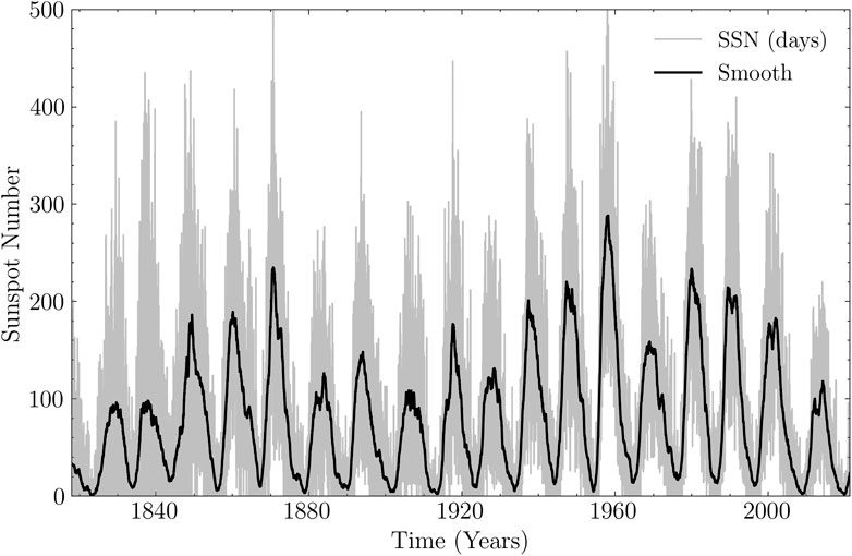
Figure 1. The sunspot numbers start in January 1818 and end in April 2021. The grey line is the raw daily average; the black curve is the result after smoothing with the Savitzky-Golay filter; the X-axis is the time, and the Y-axis is the number of sunspots counted.

The sunspot number constitutes a time series, and the process of estimating future values based on historical observations is referred to as time series forecasting. This forecasting task can be classified into two primary methodologies: single-step and multi-step. In single-step prediction, the time series is segmented into equal time intervals to predict the value at the next time step. For example, using the time series $\left\{X_t,t\in [0,n]\right\}$ to forecast $X_{n+1}$. Multi-step prediction forecasts values at multiple future time steps. To illustrate, after predicting $X_{n+1}$ using the time series $\left\{X_t,t\in [1,n]\right\}$, the next task would be to forecast $X_{n+2}$ using $X_{n+1}$. This approach enables predictions at any time step, with the step size corresponding to the number of iterations. It is essential to recognize that prediction errors accumulate in multi-step forecasting as the number of steps increases. As a result, the accuracy of multi-step forecasts tends to diminish progressively. In contrast, single-step forecasting does not experience this accumulation of error. Researchers such as Timoshenkova and Safiullin (2020) and Wang et al. (2021) have highlighted that for medium-to long-term forecasts, single-step predictions often yield greater accuracy compared to multi-step forecasts.

This research constructed three datasets for single-step forecasting of sunspot numbers over the next 12 years, each using a different length of historical data: 48, 42, and 36 years. An additional monthly average sunspot numbers dataset was constructed using the same methodology during the model validation phase. Since forecasting models primarily operate at a monthly temporal resolution, we also evaluated our model using a monthly resolution for consistency. We employed the same dataset as a benchmark across all models to ensure a fair and unbiased comparison.

3 Network construction

A GAN framework comprises two adversarial neural networks: a generator, responsible for producing new data samples, and a discriminator, which assesses these samples to differentiate between authentic and generated data. To address the challenge of non-convergence in training results within the original GAN framework, Arjovsky et al. (2017) proposed a variation known as the Wasserstein GAN (WGAN). WGAN replaces the Jensen-Shannon divergence used in the original GAN with the Wasserstein distance, modifying the objective function to improve training stability. This adjustment effectively addresses common issues in GAN training, such as mode collapse and vanishing gradients. In this study, the generator is implemented as an LSTM to produce forecasted time series data, while the discriminator is a 2D CNN that compares the LSTM-generated time series with observed data for evaluation.

3.1 The structure of the generator and discriminator

LSTM is an advanced form of Recurrent Neural Network (RNN) specifically designed to address the challenges of gradient vanishing and exploding, which frequently occur during the training of long sequences. LSTM consists of multiple cell units, each containing three gates: the input gate, the output gate, and the forget gate, as shown in Figure 2. These gates regulate the flow of information, enabling the cell to maintain and update relevant information while mitigating the impact of irrelevant or redundant data.

$•$ The forget gate, denoted as $f_t$, determines whether the previous cell state should be retained or forgotten.

$•$ The input gate, denoted as $i_t$, controls which information should be incorporated into the cell state.

$•$ The output gate, denoted as $o_t$, governs the information that should be output based on the current cell state.

Figure 2

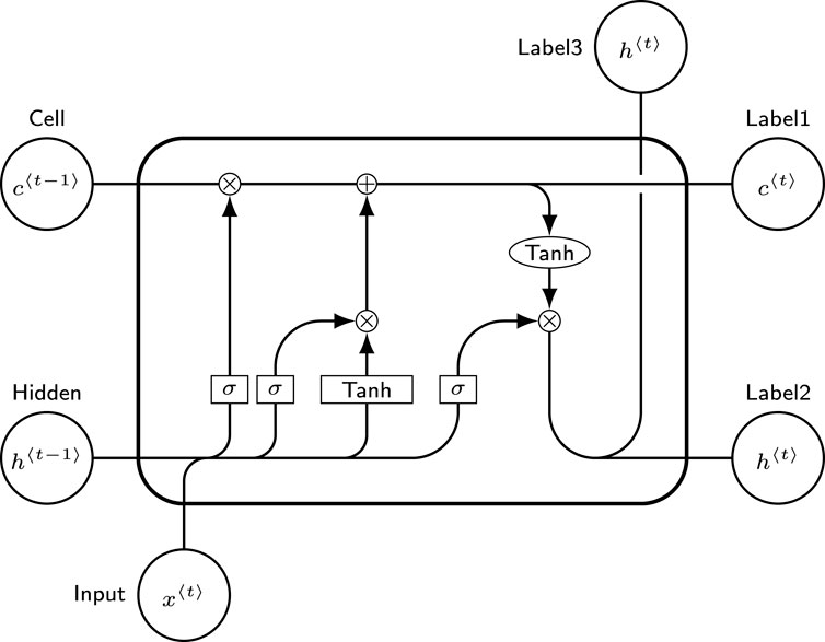
Figure 2. The structure of each cell of the LSTM. The symbol “$\otimes$” in the picture stands for the gate structure in the mathematical sense, indicating that the corresponding elements in the matrix are multiplied together. From left to right, the three gate structures are the forget gate, the input gate, and the output gate. The symbol “$\oplus$” indicates that the corresponding elements of the matrix are added together. “$\sigma$” and “tanh” represent the activation functions.

The cell state $c^{⟨t⟩}$ is influenced by both the forget gate $f_t$ and the input gate $i_t$. The current cell state $c^{⟨t⟩}$ is determined by combining the previous cell state $c^{⟨t-1⟩}$ with a modified input ${\tilde{c}}^{⟨t⟩}$. The modified input ${\tilde{c}}^{⟨t⟩}$ is calculated by applying the hyperbolic tangent function (tanh) to a weighted sum of the previous hidden state and the current input, along with a bias term. The output gate $o_t$ and the cell state $c^{⟨t⟩}$ both contribute to the computation of the predicted value $h^{⟨t⟩}$. This predicted value is obtained by multiplying the output gate $o_t$ with the hyperbolic tangent of the cell state $c^{⟨t⟩}$. The gate structures within an LSTM network enable it to effectively retain relevant information from time series data, helping to overcome the challenges of vanishing and exploding gradients commonly faced by traditional RNN networks. The main parameters of the LSTM are shown in Table 1. The input data length (time win) is $365*$48, with 1 feature. This data is first transformed into a time series with an input size of $365*$2 and a sequence length (seq len) of 24, meaning it is converted from ($365*$48, 1) to (24, $365*$2). The hidden size of each LSTM unit is $365*$6, an empirical parameter of similar magnitude to the input size. Finally, the forecasted sequence length (pre win) is $365*$12.

Table 1

Table 1. The essential hyperparameters of the LSTM network.

CNN are a class of deep learning algorithms characterized by convolutional operations and hierarchical structures. In this study, a two-dimensional convolution is used to construct the discriminator network. The process starts by transforming the time series data into a two-dimensional representation, allowing a convolutional kernel to process the data across the entire “image.” This transformation facilitates the effective handling of one-dimensional time series data within the CNN framework. Figure 3 illustrates the process of concatenating the observed data with the predicted data and then transforming it into a two-dimensional array. As shown in Figure 4, the kernel$(K)$, which matches the dimensions of the two-dimensional representation, moves through the data, generating a one-dimensional array. This array is then passed through a fully connected layer that evaluates the time series data and classifies it as “True” or “Fake.” The discriminator, essentially a two-dimensional CNN, operates as a binary classifier.

Figure 3

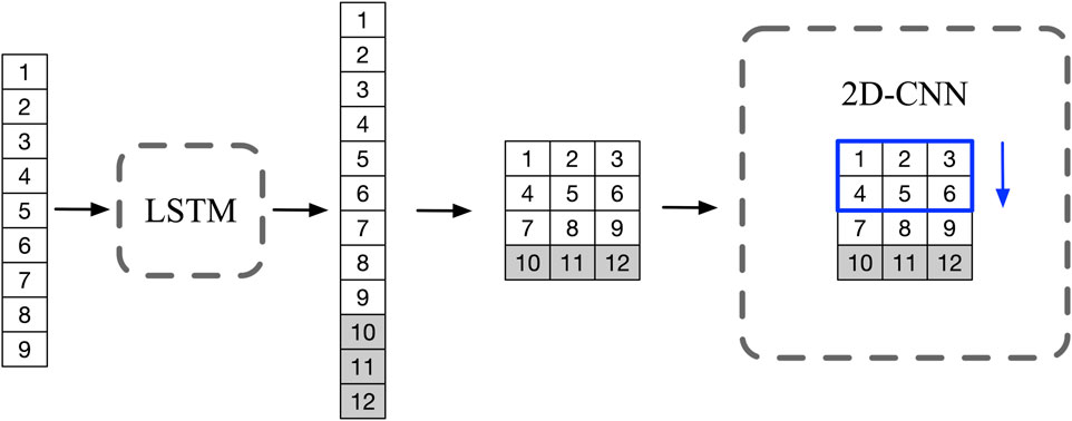
Figure 3. Schematic: The LSTM generates prediction data of length 3 ($365*$12) based on observation data of length 9 ($365*$48). These are then concatenated and transformed into a two-dimensional array with length 3 (365) and width 4 (48 + 12). The convolutional kernel has a length of 3 (365) and a width of 2 (with various kernel specifications ranging from 2 to 18). (The numbers in parentheses correspond to using 48 years of observation data to forecast 12 years of future data.)

Figure 4

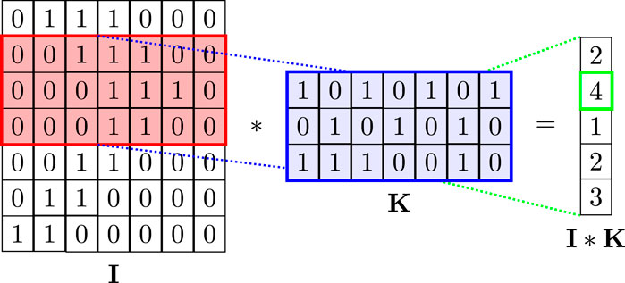
Figure 4. Schematic diagram of a two-dimensional CNN. The convolutional kernel “K” has the same length as the 2D data “I” and is available in various widths. The figure shows a convolutional kernel of width 3. Kernel “K” sweeps through “I” from top to bottom and does the convolution operation to obtain a one-dimensional array “I*K”.

3.2 The training of GAN networks

The training procedure involves two primary stages, with the initial stage focusing on training the discriminator network. In this phase, observed data are labeled as “real,” while data generated by the generator are labeled as “fake”. These data are then presented to the discriminator, enabling it to refine its ability to differentiate between them. This process is depicted in Figure 5. In the second stage, data produced by the generator is labeled as “real” and subsequently fed into the discriminator network. This stage challenges the generator to produce data capable of deceiving the discriminator. As the training progresses, the discriminator’s ability to distinguish between real and generated data and the generator’s ability to create accurate data are continuously improved. This iterative process establishes a competitive dynamic between the discriminator and the generator, ultimately driving them toward a Nash equilibrium.

Figure 5

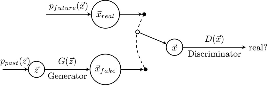
Figure 5. Network Architecture: LSTM is the generator, and CNN is the discriminator. The observed data is labeled as “real,” while the generated data is labeled as “fake”, both are presented to the discriminator to distinguish between the real and fake samples.

This approach, known as adversarial training, utilizes the interaction between the discriminator and generator networks to enhance the model’s overall performance. During this iterative training process, the discriminator becomes more effective at distinguishing between real and generated data. At the same time, the generator improves its ability to produce data that is close to real data. This adversarial training framework enhances generative models, generating more accurate and realistic data. It is essential to recognize that in the context of WGAN if one of the networks is significantly stronger than the other, it can hinder the effective updating of parameters in the weaker network. This imbalance in the capabilities of the two networks can disrupt the equilibrium and negatively affect the learning dynamics between the discriminator and the generator. As a result, the weaker network may not receive the necessary updates for optimal training. To address this challenge, it is crucial to carefully balance both networks’ strengths and capacities during the WGAN training. In this work, two methods are used to address the imbalance between the generator and discriminator in the WGAN model. First, the RMSprop optimizer improves stability by adapting the learning rate and smoothing gradients. Second, weighting the loss terms ensures a balanced contribution from both networks, making training more stable and preventing large performance differences.

Additionally, the accuracy of single-step predictions in LSTM networks is higher than that of multi-step predictions. This difference can be attributed to the accumulation of errors and noise during multi-step predictions, resulting in less accurate outcomes. Therefore, in this study, we opted for a single-step prediction approach, which allowed us to forecast sunspot numbers for the next 12 years using only one prediction step.

4 Simulation results

In this section, the model forecasting performance was first evaluated by predicting the monthly average sunspot numbers. Subsequently, the forecast results from our model were objectively compared with those generated by other well-established forecasting models. For comparison, we used forecast results available on the European Space Agency (ESA) website (https://swe.ssa.esa.int/gen_for). These results, updated monthly, covered the period starting 1 September 2016, and provided predictions for the following 12 months. It is important to clarify two aspects regarding these forecast results. Firstly, new forecast results for the next 12 months are released monthly. Secondly, we consider the forecasted values for a specific month at their initial release as the model’s forecast value.

To ensure a fair and unbiased comparison of forecast results across different models, we imposed certain constraints on the outcomes generated by our LSTM-WGAN model. Firstly, we employed the LSTM-WGAN network to forecast the monthly average sunspot numbers for 12 months. Secondly, we applied the same data extraction process to the forecasted results obtained from the LSTM-WGAN model. Lastly, we selected the period from “2016–09″ to “2023–03″ for the comparison, encompassing all the forecast results provided by ESA. The MAE between each model and the observation data is calculated for each month, followed by an analysis of these errors using Kernel Density Estimation (KDE). It is a statistical method that estimates the probability density distribution of data through a smoothing kernel function, providing an intuitive visualization of the central tendency and distribution shape of the errors. As shown in Equation 2, $\widehat{f}(x)$ represents the estimated probability density function, where $n$ denotes the number of data points, $h$ signifies the bandwidth controlling the degree of smoothing, and $K(\cdot )$ is the kernel function used for data smoothing.

$\widehat{f}\left(x\right)=\frac{1}{nh}{\displaystyle \sum _{i=1}^n}K\left(\frac{x-x_i}{h}\right)(2)$

As shown in Figure 6, the forecast results from LSTM-WGAN exhibit improved stability, with less fluctuations, and are closer to the smoothed observed data. On the other hand, the MAE of LSTM-WGAN are closer to zero and relatively concentrated. The error values of these models are presented in Table 2. Considering these aspects, the LSTM-WGAN model performs better than the other forecast models mentioned in this study.

Figure 6

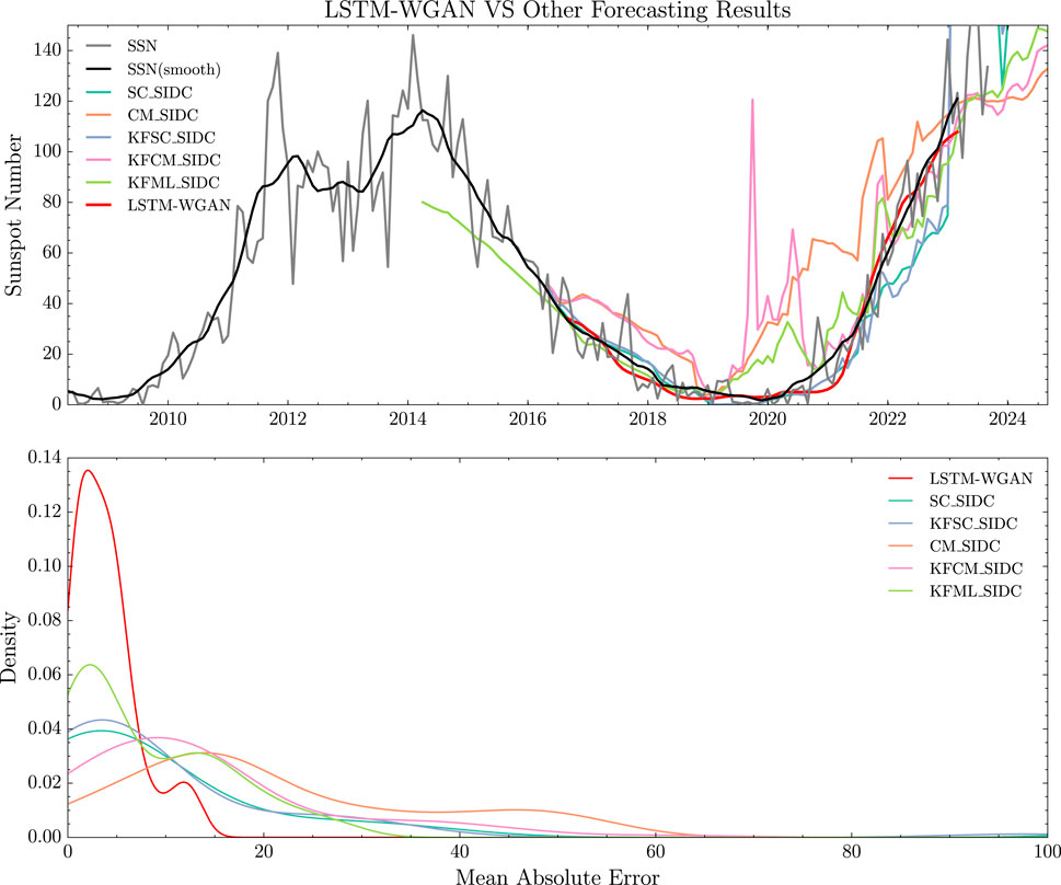
Figure 6. The upper panel of the figure, the black curve depicts the smoothed sunspot numbers, while the gray curve shows the unsmoothed sunspot numbers. The red curve illustrates the forecasted results from the LSTM-WGAN model, and the curves of other colors represent the forecasted results from various models (see Table 1). In the bottom panel of the figure, the x-axis indicates the Mean Absolute Error (MAE) between the model results and the observed results; the y-axis displays the Gaussian kernel density.

Table 2

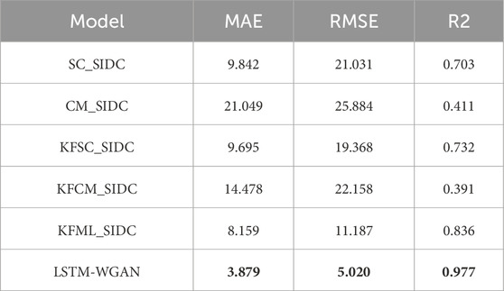
Table 2. The errors between the predictions of multiple models and the monthly average sunspot numbers were calculated. The error analysis was performed using data from September 2016 to March 2023. The table primarily presents the Mean MAE, Root Mean Square Error (RMSE), and coefficient of determination (R2). SC stands for the Standard Curves method, CM stands for the Combined method, KFSC stands for the Standard Curves method with adaptive Kalman filter, KFCM stands for the Combined method with adaptive Kalman filter, and KFML stands for the McNish and Lincoln method with adaptive Kalman filter.

Following the validation of the forecasting performance, we trained the LSTM-WGAN network using a daily average sunspot dataset to predict sunspot numbers for the 25th solar cycle. The daily average dataset offers more data than the monthly average dataset, enabling the LSTM-WGAN model to leverage its strengths more effectively. The LSTM-WGAN was tested in the 24th solar cycle. Figure 7 demonstrates that the predictions generally higher the smoothed values of the sunspot number. The results indicate better performance in the declining phase than in the ascending phase. During the peak region, the predicted values tend to exceed the smoothed values.

Figure 7

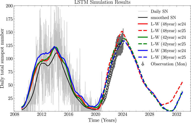
Figure 7. The solid red curve in the graph depicts the forecasted sunspot numbers for the 24th solar cycle, generated by the LSTM-WGAN model trained on a 48-year dataset. The red dashed curve represents the forecast for the 25th solar cycle. In addition, the blue and green curves show the results obtained from using 42-year and 36-year datasets, respectively.

We compared the MAE errors between various models and observational data during the ascending phase of Solar Cycle 25. The data range spans from January 2021 to October 2023. We resampled the LSTM-WGAN forecast results to monthly averages, then compared them with other models. The errors for each month were calculated and a box plot was generated. As shown in Figure 8, the accuracy of the LSTM-WGAN forecast results is significantly higher than that of the other models, with more concentrated errors, indicating that the forecast results are more stable.

Figure 8

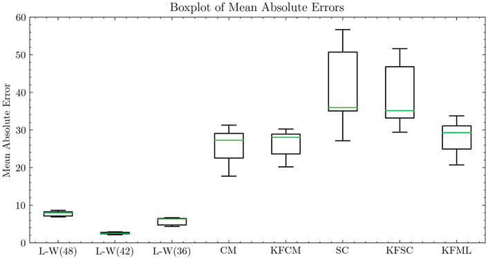
Figure 8. The error distribution from models, with the median (green) representing the central error value, while the size of the box shows the interquartile range (IQR), and the whiskers indicate the range of errors.

The larger prediction bias with 48 years of historical data may come from the complexities and periodic changes in long-term data. Although 48 years provide more reference, longer history can add noise, especially when solar activity trends are complex. In contrast, 42 and 36 years of data may focus better on the current solar cycle, improving accuracy. In theory, longer historical data should reduce prediction errors, but in practice, some uncertainties can still affect the results.

The results for RMSE and R2 between the predicted and observed data for the 24th solar cycle, based on the smoothed daily average data, are illustrated in Figure 9 (since the maximum and minimum errors of MAE differ by three orders of magnitude, RMSE is a more appropriate metric for evaluating overall error). The formula for calculating R2 is shown in Equation 3, where $y_i$ is the observed value (actual value), ${\widehat{y}}_i$ is the predicted value, $\bar{y}$ is the mean of the observed values, and n is the number of data points.

$R2=1-\frac{{\sum }_{i=1}^n{\left(y_i-{\widehat{y}}_i\right)}^2}{{\sum }_{i=1}^n{\left(y_i-\bar{y}\right)}^2}(3)$

Figure 9

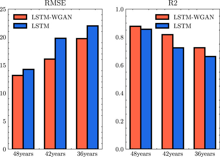
Figure 9. The red indicates the error between the LSTM-WGAN model and the smoothed sunspot number, while the blue represents the error between the LSTM model and the smoothed sunspot number. The left side of the figure displays the RMSE, and the right side shows the coefficient of determination R2.

As historical data input decreases, the difference between the predicted and observed results tends to increase. Furthermore, the LSTM-WGAN model exhibits enhanced forecasting accuracy relative to the LSTM model.

Comparing this result to other studies presents challenges. Firstly, this work employs a dataset of daily average sunspot numbers, which differs slightly from the monthly average sunspot numbers predominantly used in other research. Furthermore, this paper forecasts sunspot numbers for the next 12 years in a single step, differentiating it from different studies. In a study by Dang et al. (2022), deep learning models were compared with traditional non-deep learning models. The SARIMA model achieved an MAE of 45.51 and an RMSE of 54.11. The LSTM model achieved an MAE of 39.44 and an RMSE of 46.14, while the Informer model demonstrated the lowest errors with an MAE of 22.35 and an RMSE of 29.90. NASA’s forecasts yielded an MAE of 38.45 and an RMSE of 48.38. Similarly, in a study by Pala and Atici (2019), the RMSE for the ARIMA model was 42.41, whereas the LSTM model achieved an RMSE of 35.9. The studies by Arfianti et al. (2021) and Prasad et al. (2022) achieved better results. However, they did not compare their results with those, as they encountered difficulties achieving long-term forecasts. Their multi-step forecasts were mainly based on current observations. In general, it has been observed that as the prediction timeframe extends, the difference between the forecasted values and the actual values tends to increase.

5 Summary

This study utilized a WGAN-based neural network to forecast sunspot numbers for the 25th solar cycle. The discriminator in this network is a 2D CNN that assesses the difference between the predicted data and observations. Its primary function is to optimize the generator, which is the main component responsible for predicting sunspot numbers. The LSTM is utilized as the generator in this study due to its ability to effectively extract features from time series data for prediction purposes. Furthermore, the accuracy of single-step predictions using LSTM surpasses that of multi-step predictions. Considering these factors, the network generates a 12-year time series of sunspot numbers by constructing the dataset and tuning the parameters of both the generator and discriminator. The LSTM-WGAN model has demonstrated superior performance and higher forecasting accuracy when compared directly with the results provided by ESA. Our training involved using daily average sunspot number datasets to predict sunspot numbers for the entire solar cycle. We found that as the amount of historical input data decreases, the accuracy of the forecasts also diminishes. Additionally, the LSTM-WGAN model outperforms the standard LSTM model in accuracy. Furthermore, the predicted peak sunspot number for the 25th solar cycle is expected to be slightly higher than that for the 24th solar cycle.

Data availability statement

The original contributions presented in the study are included in the article/supplementary material, further inquiries can be directed to the corresponding author.

Author contributions

HY: Conceptualization, Data curation, Formal Analysis, Methodology, Software, Writing–original draft. PZ: Conceptualization, Funding acquisition, Methodology, Project administration, Supervision, Writing–review and editing. KZ: Investigation, Methodology, Writing–review and editing. ZS: Formal Analysis, Writing–review and editing. ZZ: Writing–review and editing, Formal Analysis. XF: Resources, Supervision, Writing–review and editing.

Funding

The author(s) declare that financial support was received for the research, authorship, and/or publication of this article. This work is jointly supported by National Key Research and Development Program of China (grant No. 2022YFF0503904), the National Natural Science Foundation of China (grant No. 42074205), Guangdong Basic and Applied Basic Research Foundation (grant No. 2023B1515040021), Hong Kong-Macao Exchange Project of Harbin Institute of Technology, Shenzhen Key Laboratory Launching Project (grant No. ZDSYS20210702140800001).

Conflict of interest

The authors declare that the research was conducted in the absence of any commercial or financial relationships that could be construed as a potential conflict of interest.

Generative AI statement

The author(s) declare that no Generative AI was used in the creation of this manuscript.

Publisher’s note

All claims expressed in this article are solely those of the authors and do not necessarily represent those of their affiliated organizations, or those of the publisher, the editors and the reviewers. Any product that may be evaluated in this article, or claim that may be made by its manufacturer, is not guaranteed or endorsed by the publisher.

References

Abdel-Rahman, H., and Marzouk, B. (2018). Statistical method to predict the sunspots number. NRIAG J. Astronomy Geophys. 7, 175–179. doi:10.1016/j.nrjag.2018.08.001

CrossRef Full Text | Google Scholar

Arfianti, U. I., Novitasari, D. C. R., Widodo, N., Hafiyusholeh, M., and Utami, W. D. J. I. (2021). Sunspot number prediction using gated recurrent unit (gru) algorithm, 15, 141–152. (Indonesian Journal of Computing and Cybernetics Systems).

CrossRef Full Text | Google Scholar

Arjovsky, M., Chintala, S., and Bottou, L. (2017). “Wasserstein generative adversarial networks,” in Proceedings of the 34th International Conference on Machine Learning (PMLR), 214–223. Available at: https://proceedings.mlr.press/v70/arjovsky17a.html.

Google Scholar

Benson, B., Pan, W. D., Prasad, A., Gary, G. A., and Hu, Q. (2020). Forecasting solar cycle 25 using deep neural networks. Sol. Phys. 295, 65. doi:10.1007/s11207-020-01634-y

CrossRef Full Text | Google Scholar

Dang, Y., Chen, Z., Li, H., and Shu, H. J. A. A. I. (2022). A comparative study of non-deep learning, deep learning, and ensemble learning methods for sunspot number prediction 36, 2074129

Google Scholar

[Dataset] Goodfellow, I. J., Pouget-Abadie, J., Mirza, M., Xu, B., Warde-Farley, D., Ozair, S., et al. (2014). Generative adversarial nets. Advances in Neural Information Processing Systems, Editor Z. Ghahramani, M. Welling, C. Cortes, N. Lawrence, and K. Q. Weinberger. Available at: https://proceedings.neurips.cc/paper_files/paper/2014/file/5ca3e9b122f61f8f06494c97b1afccf3-Paper.pdf.

Google Scholar

Han, Z., Zhao, J., Leung, H., Ma, K. F., and Wang, W. (2019). A review of deep learning models for time series prediction. IEEE Sensors J. 21, 7833–7848. doi:10.1109/jsen.2019.2923982

CrossRef Full Text | Google Scholar

Hathaway, D. H. (2015). The solar cycle. Living Rev. Sol. Phys. 12, 4. doi:10.1007/lrsp-2015-4

PubMed Abstract | CrossRef Full Text | Google Scholar

Hathaway, D. H., and Wilson, R. M. (2004). What the sunspot record tells us about space climate. Sol. Phys. 224, 5–19. doi:10.1007/s11207-005-3996-8

CrossRef Full Text | Google Scholar

Kuznetsov, N., Popova, H., and Panasyuk, M. (2017). Empirical model of long-time variations of galactic cosmic ray particle fluxes. J. Geophys. Res. Space Phys. 122, 1463–1472. doi:10.1002/2016ja022920

CrossRef Full Text | Google Scholar

Lee, T. (2020). Emd and lstm hybrid deep learning model for predicting sunspot number time series with a cyclic pattern. Sol. Phys. 295, 82. doi:10.1007/s11207-020-01653-9

CrossRef Full Text | Google Scholar

Nymmik, R., Panasyuk, M., Pervaja, T., and Suslov, A. (1992). A model of galactic cosmic ray fluxes. Int. J. Radiat. Appl. Instrum. Part D. Nucl. Tracks Radiat. Meas. 20, 427–429. doi:10.1016/1359-0189(92)90028-t

CrossRef Full Text | Google Scholar

Pala, Z., and Atici, R. (2019). Forecasting sunspot time series using deep learning methods. Sol. Phys. 294, 50. doi:10.1007/s11207-019-1434-6

CrossRef Full Text | Google Scholar

Prasad, A., Roy, S., Sarkar, A., Panja, S. C., and Patra, S. N. J. A. i. S. R. (2022). Prediction of solar cycle 25 using deep learning based long short-term memory forecasting technique. Forecast. Tech. 69, 798–813. doi:10.1016/j.asr.2021.10.047

CrossRef Full Text | Google Scholar

Schwenn, R. (2006). Space weather: the solar perspective. Living Rev. Sol. Phys. 3, 2. doi:10.12942/lrsp-2006-2

CrossRef Full Text | Google Scholar

Shen, Z., Yang, H., Zuo, P., Qin, G., Wei, F., Xu, X., et al. (2021). Solar modulation of galactic cosmic-ray protons based on a modified force-field approach. Astrophysical J. 921, 109. doi:10.3847/1538-4357/ac1fe8

CrossRef Full Text | Google Scholar

Siami-Namini, S., Tavakoli, N., and Namin, A. S. (2018). “A comparison of arima and lstm in forecasting time series,” in 2018 17th IEEE international conference on machine learning and applications (ICMLA), 1394–1401. doi:10.1109/ICMLA.2018.00227

CrossRef Full Text | Google Scholar

Timoshenkova, Y., and Safiullin, N. (2020). The dependence of the sunspot forecast accuracy using lstm networks from number of cycles in the training set. 2020 Ural Symposium Biomed. Eng. Radioelectron. Inf. Technol. (USBEREIT). Proc., 452–455. doi:10.1109/usbereit48449.2020.9117641

CrossRef Full Text | Google Scholar

Torres, J. F., Hadjout, D., Sebaa, A., Martínez-Álvarez, F., and Troncoso, A. (2021). Deep learning for time series forecasting: a survey. Big Data 9, 3–21. doi:10.1089/big.2020.0159

PubMed Abstract | CrossRef Full Text | Google Scholar

Wang, Q.-J., Li, J.-C., and Guo, L.-Q. (2021). Solar cycle prediction using a long short-term memory deep learning model. Res. Astronomy Astrophysics 21, 012. doi:10.1088/1674-4527/21/1/12

CrossRef Full Text | Google Scholar

Wu, S.-S., and Qin, G. J. a. p. a. (2021). Predicting sunspot numbers for solar cycles 25 and 26

Google Scholar

Xu, T., Wu, J., Wu, Z.-S., and Li, Q. (2008). Long-term sunspot number prediction based on EMD analysis and AR model. Chin. J. Astronomy Astrophysics 8, 337–342. doi:10.1088/1009-9271/8/3/10

CrossRef Full Text | Google Scholar