PMODE I: Design and Development of an Observatory for Characterizing Giant Planet Atmospheres and Interiors

The giant planets of our Solar System are exotic laboratories, enshrouding keys which can be used to decipher planetary formation mysteries beneath their cloudy veils. Seismology provides a direct approach to probe beneath the visible cloud decks, and has long been considered a desirable and effective way to reveal the interior structure. To peer beneath the striking belts and zones of Jupiter and to complement previous measurements—both Doppler and gravimetric—we have designed and constructed a novel instrument suite. This set of instruments is called PMODE—the Planetary Multilevel Oscillations and Dynamics Experiment, and includes a Doppler imager to measure small shifts of the Jovian cloud decks; these velocimetric measurements contain information related to Jupiter’s internal global oscillations and atmospheric dynamics. We present a detailed description of this instrument suite, along with data reduction techniques and preliminary results (as instrumental validation) from a 24-day observational campaign using PMODE on the AEOS 3.6 m telescope atop Mount Haleakalā, Maui, HI during the summer of 2020, including a precise Doppler measurement of the Jovian zonal wind profile. Our dataset provides high sensitivity Doppler imaging measurements of Jupiter, and our independent detection of the well-studied zonal wind profile shows structural similarities to cloud-tracking measurements, demonstrating that our dataset may hold the potential to place future constraints on amplitudes and possible excitation mechanisms for the global modes of Jupiter.

1 Introduction

A fundamental question that astronomers have long struggled to answer is that of the formation of our Solar System—did the planets build up from the core accretion process occurring in the protoplanetary disk, or did they collapse down from gravitational instabilities in the gas of the disk, similarly to stellar formation? One way to distinguish between these competing formation theories is by revealing the deep internal structure of the Gas Giants, specifically the radial distribution of heavy elements—is a solid core present deep within the gaseous envelopes, and if so, is it compact or diluted? The presence of a solid core (whether the boundary be defined or diffuse) perhaps entirely refutes the disk instability formation theory, as diffusive settling of heavy elements into the central region of a planet from an originally homogeneous radial distribution would require a timescale longer than the current age of the Universe, for a planet with Jovian mass and radius. If the additional impact of mixing by convection is considered, this timescale becomes even longer (Stevenson, 2020).

To date, the interiors and atmospheres of Jupiter and Saturn have been probed by measuring gravitational moments using spacecraft passing close to or in orbit around the planet. These measurements are combined with our best understanding of the thermodynamics and energy transport in the planets to provide estimates of how the density and temperature vary with radius. However, there are several limitations associated with using gravitational moments as probes of the planet’s deep interior. Due to the nature of the observations, constraints provided by gravity field measurements are localized to the outer regions of the planet (Guillot (2005), Figure 4).

Models which fit observations of the well-constrained outermost regions of Jupiter suggest that there exists a heavy-element core with a diluted boundary deep within the planet, containing ∼5–15% of the Jovian mass, and extending to nearly half of Jupiter’s radius (Wahl et al. (2017); Liu et al. (2019)). Unfortunately, this is around the same radius where gravimetry measurements lose the majority of their sensitivity (Helled et al., 2010), leaving the interior structure of Jupiter fully model-dependent. Thus, a different type of measurement is needed to probe the inner 50% of Jupiter’s radius to further constrain the deep internal structure of the planet and compliment Juno’s measurements.

In addition to constraining the properties of the Jovian core, measurements capable of probing the inner regions of the planet will also provide further information on the Jovian atmospheric dynamics. Jupiter’s zonal wind profile—obtained by averaging the winds circulating from east to west over longitude and recognized as a fundamental constraint of the Jovian atmosphere (Ingersoll et al., 2004)—has been studied extensively via cloud-tracking measurements (Hubble, Voyager, ground-based, etc.), which are based upon feature-tracking of the visible cloud decks through time. However, cloud-tracking fundamentally maps the motion of large structures, and thus provides information on the velocity of iso-pressure regions as opposed to the true cloud particle velocity; this measurement could drastically differ for cases such as disruption of cloud structure by atmospheric gravity or thermal waves. Thus, it is desirable to find an alternative method to confirm and validate cloud tracking measurements.

The zonal wind profile below the cloud level has been studied via temperature measurements in the IR (though these measurements directly make use of the cloud-tracking profile (Fletcher et al., 2016)) and through gravimetry (Juno), but many questions still arise. To what depth do these zonal winds reach? Are they maintained by thermal convection reaching deep into Jupiter’s interior, or are they caused by temperature differences between the striking belts and zones, constraining the wind to a thin, surface-level weather layer? This is a question that has sparked interest for nearly three decades (Dowling, 1995), and was a key question intended to be answered by measurements taken with the Juno spacecraft (Hubbard, 1999). Recent results from gravimetry measurements from Juno revealed a north-south asymmetry in the gravity field, which can only be due to atmospheric dynamics. The odd harmonics J₃ to J₉ as measured by Juno have been used to measure the zonal wind profile to a depth of ∼3,000 km, a region containing ∼1% of the Jovian mass, and show that the gravimetry measurements suggest that the wind flow at this depth is strongly correlated with the visible flow of the clouds (Kaspi et al., 2018). However, the solution to the gravimetry inversion problem is fundamentally non-unique (different zonal wind profiles may provide similar gravimetry signals), and thus, model dependent. In fact, it has been shown that both the shallow and deep interior flow models for the Jovian zonal winds can produce the odd J-component measurements collected by Juno (Kong et al., 2018). Further direct measurements of these zonal flows, as are possible via Doppler velocimetry, will compliment those collected by Juno, provide more detailed information on the coupling between surface-level and interior wind flows, and help determine the origin of the Jovian winds.

A second atmospheric dynamics question which remains to be answered is: how does this profile vary over time? Globally, the zonal wind profile appears to be exceptionally stable (velocities on the order of 150 ± 10 m s⁻¹), but locally, some regions show year-to-year variation, on which further observations are desired to confirm the current leading theories. The Northern Equatorial Belt (NEB, the band located around 7°N) shows cyclical variation on the order of ∼4 years, which is a known location of plumes and hot spots coupled with dark projections that show characteristics of a trapped planetary-scale Equatorial Rossby wave (Arregi et al., 2006; Barrado-Izagirre et al., 2013). The horizontal components of these features at a surface level can be measured via cloud-tracking, but discerning vertical components adds an additional level of complexity. Simulations show that these hot spots should develop vertical shear on the order of 70 m s⁻¹ (Showman and Dowling, 2000). Additionally, the Northern Temperate Belt (NTB, the band located around 21°N) shows year-to-year variation, caused by high-albedo plume outbreaks which occur every ∼5 years (the most recent published occurrence happened in 2016) and create strong features encircling the planet (Sánchez-Lavega et al., 2017). It has been recognized that, in addition to model-based approaches, continued monitoring through of these quasi-periodic outbreaks and temporal changes has the potential to offer insight into the changing balance between circulation cells and the quasi-periodic events which trigger the changes (Fletcher et al., 2020b). Further constraining the structure of the winds is paramount to further understanding not only the causes and effects of these planetary scale disturbances, but of the origin of the global Jovian circulation (Ingersoll and Pollard, 1982).

Doppler velocimetry has long been considered both for the search of planetary oscillations (e.g., Vorontsov et al. (1976); Schmider et al. (1991); Schmider et al. (2007); Gaulme et al. (2011)) and for measuring atmospheric dynamics, for example with the moons Io and Titan (Civeit et al. (2005); Luz et al. (2005); Luz et al. (2006)) or Venus (e.g., Lellouch et al. (1994); Machado et al. (2017); Gaulme et al. (2019), and references therein). The best approach to track the atmospheric motions in the visible domain—vertical for seismic observations, horizontal for wind circulation—consists of measuring the Doppler shift of Solar Fraunhofer lines that are reflected by the planet’s upper cloud layers, as the Doppler signal is enhanced by reflection (e.g., Gaulme et al. (2018)). In regards to the seismology of giant planets, all attempts have been dedicated to Jupiter because it is the biggest and brightest target as seen from Earth. First observations with a magneto-optical filter (MOF, Cacciani (1978)) were led by Schmider et al. (1991), then followed by observations with a Fourier-transform spectrometer (Mosser et al. (1993); Mosser et al. (2000)), a double MOF (Cacciani et al., 2001), and with the first dedicated instrument SYMPA (Schmider et al. (2007); Gaulme et al. (2008); Gaulme et al. (2011)), a Fourier transform spectrometer too. Observations by Schmider et al. (1991), Mosser et al. (1993), Mosser et al. (2000), and Gaulme et al. (2011) concluded on the presence of oscillations at a low signal-to-noise level, with amplitudes between 0.1 and 1 m s⁻¹. In regards to atmospheric dynamics, most of the efforts were dedicated to Venus, in particular, to support the ESA Venus Express mission (Lellouch and Witasse, 2008). Venus observations were mostly performed by scanning the planet with a single-fiber fed high-resolution spectrograph (e.g., Widemann et al. (2008); Machado et al. (2017), or with long-slit spectrographs (Machado et al. (2012); Gaulme et al. (2019)). So far, the only measurements of Jupiter’s zonal wind profile were performed with the dedicated instrument JOVIAL, inherited from SYMPA by Gonçalves et al. (2019). Finally, we note that Doppler spectrometry has even been utilized to conduct wind velocity measurements of exoplanets (Louden and Wheatley (2015), Brogi et al. (2016).

In this paper, we report the results of the first observations of the newly designed set of instruments called PMODE—the Planetary Multilevel Oscillations and Dynamics Experiment. This project is built upon the experience and history of using MOFs for seismic observations of the Sun (helioseismology). The ultimate goal of the instrument is to be mounted at South Pole for continuous observations of Jupiter during the polar night. Along the route to achieving this ultimate goal, we were granted 45 nights on the 3.6-m AEOS telescope located at Mount Haleakalā, Maui, HI, during which we obtained 23 nights with good weather. The objective of this first paper is to present the PMODE instrumentation and capabilities, including on-sky validation of Doppler velocity measurements in the form of a preliminary measurement of the well-studied zonal wind profile of Jupiter. A thorough analysis of the data for a detailed comparison of the PMODE zonal wind profile with previous works, as well as investigation of the data for seismic purposes is under development and is left for a future paper. We detail first the instrument principle and theoretical performance (Section 2), the observations (Section 3), and our instrumental validation regarding the zonal wind profile as well as a preliminary search for oscillations (Section 4).

2 PMODE: The Planetary Multilevel Oscillations and Dynamics Experiment

2.1 Instrumental Concept

Radial velocity shifts of the reflected light from Jupiter’s cloud decks can be measured using a Doppler imager. This type of instrument has been used extensively in helioseismology due to the underlying performance of the narrow passbands (∼40 mA) created by the MOF system. The passband configuration leads to a scenario where both sensitivity and a wavelength stability of 0.0015 mÅ, or ∼6 cm s⁻¹ (Tomczyk et al., 1995) allow for very precise velocimetric measurements. MOF-based approaches have proven to be extraordinarily successful in mapping out the interior structure of the Sun and other stars (asteroseismology). In terms of planetary seismology—or Dioseismology, in the particular case of Jupiter—the Doppler imager views reflected sunlight off of Jupiter’s cloud decks through two very narrow passbands in the wings of a strong Solar absorption line (Agnelli et al. (1975); Dick and Shay (1991); Tomczyk et al. (1995)), which provides a sensitive measure of the Doppler shift of the light reflected off the Jovian cloud decks.

We have implemented this powerful tool of Doppler velocimetry in a multi-channel instrument to measure the atmospheric dynamics and oscillations of Jupiter, called PMODE: the Planetary Multilevel Oscillations and Dynamics Experiment. Our Doppler imager is designed to detect concurrent radial velocity shifts of the 589 nm sodium [probing an effective depth of ∼3 bar (Cacciani et al., 2001)] and 770 nm potassium lines [∼0.7 bar (West et al., 2004)]. In addition to the Doppler imager, there is a polarimetric channel that measures the linear polarization of light reflected off the Jovian clouds. This channel increases spatial coverage on the disk of Jupiter while also maximizing scientific return by utilizing a larger portion of the collected light. Simultaneous information on the Jovian atmosphere at levels probed by the 889 nm methane band [∼0.2 bar (West et al., 2004)] may also prove to be a valuable diagnostic in the future. Within the Doppler imager, we theoretically have the capability to concurrently probe two separate atmospheric levels of Jupiter, providing the ability to collect three-dimensional measurements. In this paper, we focus on the full design of the instrumentation, but scientific validation and results are discussed specifically and exclusively the for the potassium channel of the Doppler imager side of the instrument. Discussion and analysis of both the sodium Doppler imager channel (unfortunately plagued by detector artifacts, which have as of yet prohibited analysis of the collected data) and the polarimeter channel will be considered in a future work.

PMODE was originally designed with the intent of deploying to the geographic South Pole over the Austral winter of 2021; details specific to this original design (hereafter referred to as LANDIT: the Long-duration Antarctic Night and Day Imaging Telescope) will be discussed in a future paper within the PMODE series. This paper discusses the redesign and modification of the LANDIT instrument for use on a large aperture telescope, and specifically focuses on the details for solely the potassium channel of the Doppler imager.

2.2 PMODE: The Doppler Imager Channels

Our Doppler velocimeter is designed to map the line of sight velocity of flows and waves in the tropospheres of Jupiter by measuring Doppler shifts in reflected solar Fraunhofer lines: the two sodium D lines at 589.0 and 589.6 nm (combined as a single measurement channel, yet unfortunately complicated by detector artifacts—however, we find it important to discuss the design of this channel regardless), and the potassium D₁ line at 770 nm. Our instrument utilizes these two MOFs to produce narrow pass-bands in the wings of the target lines, which can be used to resolve the reflected solar line, thus allowing for high-sensitivity Doppler shift estimates to be made.

Figure 1 displays a representative diagram showing the path of light through our MOF channels, which utilize a single-cell design [as detailed in Cacciani et al. (2001)] as opposed to the instruments used for helioseismology, where the Doppler measurement is obtained by differential measurement of the two wings in the line. Instead, PMODE uses only one line transmission profile, compared to the continuum, where our sensitivity to the Doppler shift is obtained in the wings of the spectral transmission profile. In this figure, light enters from the left via a narrow-band pre-filter (2 nm for sodium and 3 nm for potassium), then passes through a polarizer, which allows only light matching the orientation of the polarizer to pass. This light then passes through a heated glass cell containing potassium or sodium vapor. A permanent magnet assembly applies a magnetic field to the cell, parallel to the optical path. This magnetic field causes the polarization state of the light to change in the wings of the K or Na resonance lines, primarily via Faraday rotation. Light passing through the cell then encounters a second polarizing element (this time, a Wollaston prism), orthogonal to the first. At this Wollaston, each beam is split into two diverging beams, one beam passes unattenuated, the other is blocked, apart from the narrow passband where the polarization has been rotated. This results in two beams that produce two images on the CCD, one of which is of the 2 or 3 nm continuum, the remaining is of the MOF passband, hereafter referred to as the “MOF image.” The ratio of the MOF image to the continuum image provides a sensitive measure of Doppler shift to produce the final data product: radial velocity map called a Dopplergram, which is insensitive to albedo fluctuations. Within this Dopplergram, any intensity changes should theoretically only be due to the Doppler shift of the light.

FIGURE 1

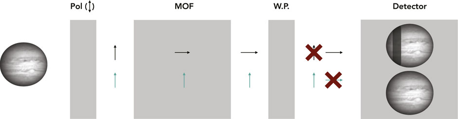
FIGURE 1. Visualization of the path of light through a MOF located between two crossed polarizers. The black arrows represent light in the wings of the absorption line, while the green arrows represent the continuum portion of light outside of the absorption line. The light first passes through a vertically oriented polarizer, then into the heated vapor cell enclosed in a permanent magnet assembly, applying a magnetic field parallel to the optical path. 1) The light in the wings of the absorption line (black arrow) experiences a rotation of its polarization state, allowing it to pass through the final polarizer (a Wollaston prism), which separates the vertical and horizontal polarization states and projects them onto the detector, where the absorption line profile is now visible on the “velocity” or “MOF” image. 2) The continuum portion of light (green arrow) is unaffected by Faraday rotation within the MOF and passes unattenuated through the MOF and the Wollaston prism, maintaining its original vertical polarization state and thereby producing a “continuum” image on the detector.

The instrument’s velocity signal (shown in Figure 2) manifests as a tracing of the absorption line of interest projected onto the Jovian disk. This comes as a result of the MOF passband scanning the spectral range—primarily due to the rapid rotation of Jupiter. Figure 3A shows the impact of this rotation on a K 770 nm MOF image—the Solar line seen by this channel, convolved with the filter passband, is much narrower than the equatorial Doppler shifts caused by Jupiter’s rotation, and so the line is resolved in the image, and seen as a dark band parallel to Jupiter’s spin axis. While this provides high local sensitivity, much of the surface of Jupiter is Doppler shifted out of the instrument’s spectral range. This exacerbates spatial aliasing, making it more difficult to identify specific modes. In our Doppler imager, we attempt to alleviate this problem by utilizing a second channel that passes the two Na D lines at 589 nm. The Na lines are much broader, providing Doppler sensitivity out to the planetary limb (Figure 3B), and together with the K 770 nm, provide good sensitivity over the entire disk, as is seen in Figure 3C. Output images (MOF image, continuum image, and resultant Dopplergram) collected with this instrument package on the AEOS telescope over the course of a 24-day observing run and processed through our MATLAB data reduction pipeline (which applies bias-, dark- and flat-field corrections, further detailed in Section 4) are shown in Figure 2.

FIGURE 2

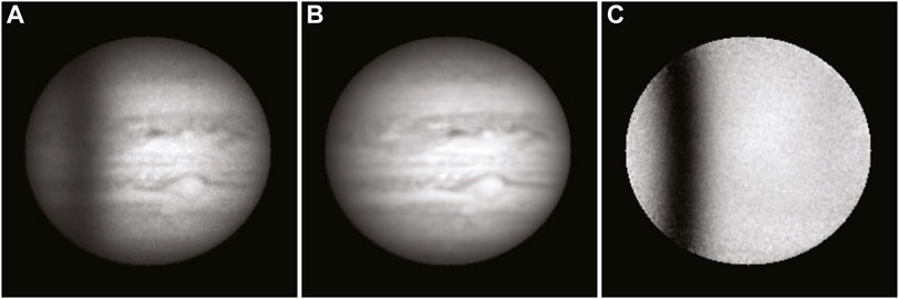
FIGURE 2. (A): “velocity” or “MOF” image, displaying the absorption line feature near the top of the disk. (B): “continuum” image, with no velocity sensitivity, recorded simultaneously and on the same detector as the velocity image. (C): the velocity image divided by the continuum image to produce the final data product: a Dopplergram, where pixel intensity values correspond to Doppler velocities towards and away from the observer within the dark absorption band. This data was collected during the 24-day observing run on the AEOS 3.6 m telescope. Particularly, these frames are from the night of 12 August 2020, with a 13.76 km s⁻¹ relative velocity between observer and Jovian disk center. All three frames are from a single integration and have had basic data reduction steps (bias, dark, leak image, and flat-field calibration, further detailed in Section 4) applied. Each image has been normalized to its respective maximum value for ease of viewing, and each has 200 pixels across the Jovian disk.

FIGURE 3

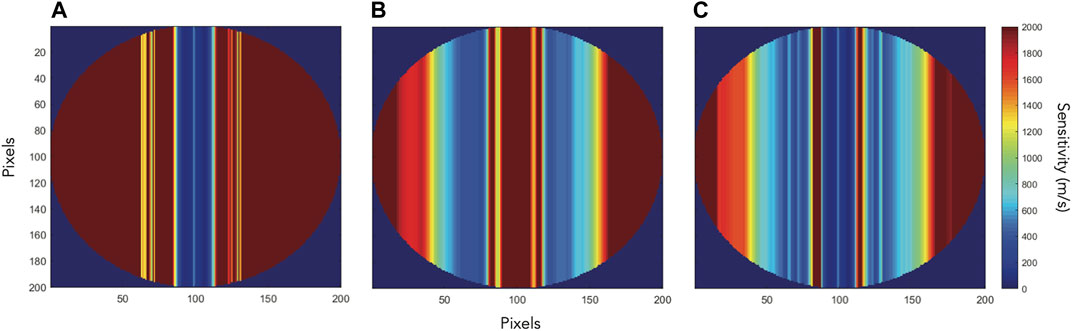
FIGURE 3. Simulation displaying sensitivity of the MOF channels of PMODE. Here, a lower value represents a higher sensitivity, as we are displaying the ability to measure smaller Doppler shifts—therefore, a sensitivity of 200 m s⁻¹ is better than a sensitivity of 2,000 m s⁻¹. These channels provide sensitivity over the majority of the Jovian disk. The 770 nm K cell provides a steeper (and thus more sensitive) line covering a smaller amount of area, while the 589 nm Na doublet has a shallower (and thus less sensitive) profile, covering a larger amount of area on the disk. Panels (A,B) show the modeled sensitivity for the K and Na cells respectively, assuming Jupiter is at opposition, while panel (C) shows the Na and K cell sensitivities combined.

Jupiter rotates rapidly with a rotation period of 9 h 55 m. This results in a Doppler velocity signal of 12.6 km s⁻¹ on each side of Jupiter at the equator. However, when viewing reflected light from the Sun-Jupiter-Earth system, a doubling effect (as detailed in Section 4.5) occurs that creates a change of ±25.2 km s⁻¹ across the sunlit side of the planet’s disk. We derive our sensitivity and velocity magnitude using an “on-planet” calibration source, utilizing the knowledge that our ∼200 pixels across the disk correspond to the ±25.2 km s⁻¹ from Jupiter’s rotation from edge to edge. This spatial extent on the detector combined with the rotation rate can be used to provide a value in $\frac{m/s}{pix}$. We then calculate the intensity change within the absorption line profile of the Dopplergram (following bias-, dark, leak-, and flat-correction, and division of the MOF image by the continuum image) corresponding to a range of pixels (we chose 15 for consistency), to obtain a value of $\frac{DN}{pix}$, with DN representing the values in the Dopplergram following all calibrations, corrections, and image division. Combining these two values provides a final calibration unit of $\frac{DN}{m/s}$. This calibration can then be divided into each pixel value to convert from DN to m s⁻¹. The final equation for calculating this unit for each night is as follows:

$VF=\frac{{\mathrm{\Delta }}_f}{R_{size}}\times \frac{Ju{p}_{size}}{4V_{Jup}},(1)$

here, VF represents our MOF unit in $\frac{DN}{m/s}$, with Δ_f representing the intensity variation along the measurement region R on the Dopplergram with size R_size (in pixels), Jup_size being the Jupiter diameter in pixels on the detector, V_Jup being the rotation velocity on Jupiter at the equator (in m s⁻¹), and the factor of 4 comes from the velocity difference at each edge of Jupiter equal to + V_Jup, and − V_Jup, multiplied by the phase factor (1 + cos ϕ), which is almost equal to two for observations from the Earth near opposition. This MOF unit varies slightly from night to night, primarily due to the shifting of the absorption line center as a function of the radial velocity between Jupiter and Earth (an effect discussed further in Cacciani et al. (2001) and Cacciani et al. (1998)) in addition to smaller second-order effects (oblateness, differential rotation, inclination, and Jovian phase, which are not considered in this first-order analysis but remain for future investigation), and is calculated accordingly each night to account for this change.

2.3 Optical Design and Modifications

PMODE was originally designed for the Cassegrain port of a 0.5 m Ritchey-Chrétien telescope, a system that was chosen for relatively simpler integration among the complex logistics of operating a telescope at the South Pole. However, for use in a Coudé room of the AEOS 3.6 m telescope, the optical layout (see Figure 4) could be preserved, but the fore-optics required a larger demagnification ratio in order to pair with the facility adaptive optics (AO) system, features of which are thorougly detailed in Roberts and Neyman (2002). Because Jupiter is an extended source, only tip/tilt compensation—as opposed to full AO compensation—was applied for simplicity. Full AO correction is applied when observing smaller targets of opportunity during the summer 2020 PMODE campaign, but we do not discuss these targets here as the primary observations of interest pertain to Jupiter.

FIGURE 4

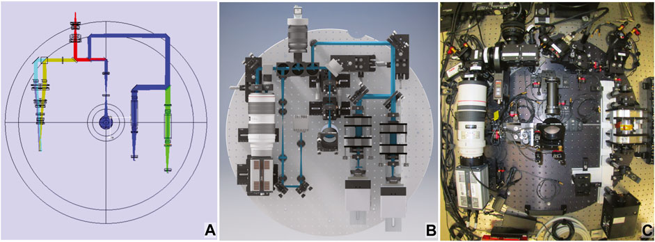
FIGURE 4. (A): A Zemax model of the complete LANDIT (the South Pole version of PMODE) focal plane instrument suite. (B): a rendered CAD drawing of the LANDIT instrument suite. The left side of the path contains the polarimeter, tracker, and wavefront sensor. The right side of the path contains the sodium and potassium MOF channels. (C): The actual system as of July 2019. Here, one channel is missing from the Doppler imager. No photographs were collected of the completed PMODE instrument, so we provide these of her sister instrument, for reference.

Figure 5 shows a schematic optical layout for PMODE. The 60 arcsecond FOV from the telescope enters the AO system (Roberts and Neyman, 2002) where the Fresnel reflection from an uncoated window is used for atmospheric tip-tilt compensation and higher order wavefront measurements when observing smaller targets besides Jupiter. A subsequent 4:1 beam reducer precedes the 1–2 inch optics of PMODE. We then split the beam at λ = 805 nm for the Doppler velocimetry (λ ∼589 and 770 nm) and polarimetry (λ∼889 nm) channels. Another dichroic further splits the beam at λ∼605 nm for the Na and K MOF channels.

FIGURE 5

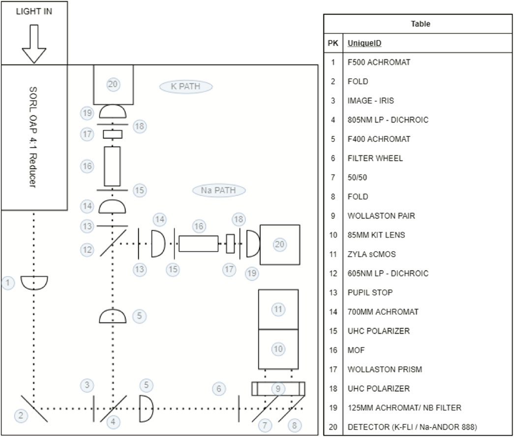
FIGURE 5. Diagram of the optical bench for the summer 2020 PMODE observational campaign. The left panel displays a top-down view of the bench. The right panel displays the name of each optical component corresponding to the numbered circle within the left panel. The light enters through the upper left of the diagram, then is split by dichroics into three separate paths. Clockwise from the top left: 770 nm potassium MOF channel, the 589 nm sodium MOF channel, and finally the 889 nm polarimeter channel follows the path along the bottom edge of the diagram.

There were a few significant optical modifications implemented within the PMODE optical path, differentiating from the sister instrument which much of our infrastructure is inherited from (LANDIT). Firstly, available relay optics for the AEOS 3.6 m experiment meant that single beam polarizers, providing a 10^–5 extinction ratio, were required to be placed in front of the MOFs, as opposed to the original optical design (which consisted of a Wollaston prism placed before the vapor cells, and provided a higher extinction ratio (approximately 10^–6) and a low cut angle to reduce optical distortion). The replacement of these optical components results in a $\sqrt{2}$ loss in SNR, but was a necessary modification to remove any scattered light throughout the vapor cells which, if left uncorrected, could manifest as a (false) apparent velocimetric signal. Secondly, and due in part to the aforementioned swapping of the original Wollaston prism for a single polarizer in front of the vapor cells, a clean-up polarizer is used after the exit Wollaston prism immediately following the vapor cells to decrease the contrast between the continuum and MOF images. This clean-up polarizer is adjusted to maximize the MOF signal, and is nearly crossed with the continuum image to drastically decrease its flux (These modifications are visualized in Figure 5.). Approximately 4° of tilt can be added to the Wollaston prisms to reduce optical distortion between the continuum and MOF images, which must be compared to retrieve the line-of-sight velocity signal. This tilting technique reduces the relative difference between the two optical paths emerging from the Wollaston prism (Simon, 1986). Finally, 2–3 nm bandpass filters define the respective image continua and are placed immediately ahead of the detectors. In PMODE, we use 1024 × 1024 CCDs with 13 μm pixels.

2.4 Theoretical Performance

Here, we look to model the instrumental velocity sensitivity of the Doppler imaging system. This simulation looks to estimate the photon noise level of Jupiter on our detector during the observational campaign, particularly for the case where a potassium vapor cell is used.

The sensitivity of the instrument is defined as the relative flux measurement produced by a Doppler shift of the absorption line. Our measurement relies on the phenomena where Solar light is reflected off of the cloud tops in the Jovian atmosphere. Any Doppler effect imparted on the line ever so slightly shifts or morphs (Cacciani, 1978) the absorption profile in relation to the stable pass-bands. Each narrow pass-band, generally some 0.004 nm in width, then measures an integrated signal that results in a relative dimming/brightening of the affected region. To mathematically describe this change in recorded flux, we look to the convolution of the derivative of the absorption line with the passbands created by the MOF:

$S=\frac{\frac{dF}{dv}*I}{F*I}(2)$

The quantity I represents the total intensity of the passband created as function of wavelength (or in this case, a function of Doppler shift). F is derived from the photon flux measured at the detector, we further describe this scenario below.

From Eq. 2, we see that the derivative of the line significantly contributes to the overall effectiveness of the technique. Solar lines that exhibit steep profiles allow for more precise measurements of relative velocity change. Conversely, wider Solar lines provide less sensitivity, but greater spatial coverage. These scenarios are valid only in the case of rapidly rotating and resolved targets—non-resolved targets with varying global effects may not exhibit the same behavior. As a first order approximation, the observational constraints can be used to produce a spatially-resolved sensitivity simulation, which allows for a preemptive determination of the instrument’s expected performance.

If Jupiter is considered to be a solid-body rotator, differential rotation is out of the scope here and contributes very little; the computed sensitivity is obtained through photometric and velocimetric analysis. The photometric analysis must include the total amount of photons received at the detector. A few quantities that are useful here include: the energy of a photon at 700 nm (2.6 × 10^–19 J), the Solar photon flux at Earth (4.65 × 10¹⁸ hv/s/nm/m²), the Solar photon flux at Jupiter (1.7 × 10¹⁷ hv/s/nm/m²), the total flux at Jupiter (2.7 × 10³³ hv/s/nm), and finally, the albedo of Jupiter at 770 nm, which is 0.46.

Next, we must account for any instrumental effects or losses. The transmission of each optical component and detector characteristics can be used to gain an understanding of the expected image to be used for further analysis. For the mode of observation used within this work, we investigate a scenario where the total transmission is ∼5% upon reaching the detector (calculated via the expected optical component transmission). Having determined the incident flux, we can now model an image of Jupiter that corresponds with the expected observations. The inclusion of resolution, average seeing, Jovian phase, and limb-darkening completes this model.

For the velocimetric component, we use the rotation rate of Jupiter coupled with the line of sight velocity to project the radial velocity sensitivity onto the disk (as described in Eq. 1). A standard sensitivity calculation is then used to produce the expected sensitivity as $S=\frac{1}{S\sqrt{N}}$. The result of this computation is what is shown in Figure 3. This analysis was adapted from techniques detailed by Gaulme et al. (2011).

From this purely theoretical photon noise analysis, the lowest attainable noise level is ∼240 m s⁻¹ per pixel, per 28-s exposure. By considering only pixels for which noise levels are lower than 1,000 m s⁻¹, the average sensitivity for all pixels meeting this criteria is 616 m s⁻¹. If we then include the sensitivity gained by summing all of the pixels, a roughly 7 m s⁻¹ sensitivity is attained per 28-s exposure.

When comparing this theoretical performance with the actual instrumental performance following on-sky calibration (as detailed in Section 3.2), we find that our true per-image noise level is comparable with theoretical estimates. Our resultant images for the K MOF channel provide a plate scale of 0.22 arcseconds per pixel; this over-samples our target by a factor of 3 while solely utilizing KHz rate tip-tilt correction (active AO compensation brings this closer to unity). The standard deviation of our true velocity signal during a 28 s exposure is equal to 332 m s⁻¹ per pixel. When we account for the number of pixels contained in the velocity-sensitive region (some 700 pixels when considering seeing), a 12.7 m s⁻¹ sensitivity is achieved per image. This per-image sensitivity yields a full time series theoretically capable of sensing near a level of 10 cm s⁻¹.

3 Observations

To study the interior dynamics and global oscillations of Jupiter with PMODE, we utilized 6 weeks of observing time on the AEOS 3.6 m telescope at Haleakalā Observatory in Maui, HI, which began in July 2020 and were centered around Jupiter at opposition. The data frames were collected on a 30-s cadence (with a 28-s exposure time and 2 additional seconds to allow for camera readout) to prevent blurring of the disk from field/feature rotation and to ensure sufficient time sampling of the Jovian oscillations. Our dataset provides an average of 200 pixels spanning the diameter of Jupiter, resulting in a theoretical spatial resolution of 0.25 arcseconds per pixel. Utilizing the full 24-day campaign provides a frequency resolution of 0.48 μHz, but we note that the extent of our observations will allow us to divide our time series into smaller, equal length segments and average the resultant power spectra from these. Averaging the spectra in this way will produce lower resolution, but will (importantly) decrease the background noise and false peaks due to the expected stochastic excitation of the modes. We note that we have the capability to choose the length of segments we split our observations into during the analysis process, and that final frequency resolution is determined by this splitting.

3.1 Observing Conditions

As gathering information on the internal structure and dynamics of Jupiter was the primary goal of this observational campaign, we prioritized collecting data on Jupiter each night, beginning at sunset and continuing until Jupiter reached an altitude of 10° above the horizon. As we observed for entire nights, the remainder of time after Jupiter set was spent observing targets of opportunity which we deemed as scientifically valuable given the capabilities of our instrument. Naturally, the most intuitive secondary target to observe would be Saturn, which is equally interesting for seismology—although it is dimmer than Jupiter and thus more difficult to obtain the desired signal in the deep absorption line band. However, during the duration of our observational campaign (July–August 2020), Saturn set roughly 30 min after Jupiter each night, rendering it unsuitable as a late-night target. Instead, we decided to focus the remainder of our awarded time primarily on Uranus, as it is a prime target of interest and much remains to be uncovered on the coupling between winds, temperatures, and clouds (Fletcher et al., 2020b), understanding of which would significantly help fill a large, unexplored regime in current understanding of atmospheres of planets with low sunlight, cool temperatures, and significant internal mixing and energy (Fletcher et al., 2020a).

Of the 45 total nights utilized, 14 of these nights were spent on instrumentation build, alignment, and on-sky calibration; 7 nights were lost to weather and site-related issues. Our total data collection time was 24 nights encompassing 6 August 2020 through 30 August 2020 (with the single night of 29 August 2020 lost to poor weather), spanning an Earth-Jupiter velocity range of 11.12 to 20.37 km s⁻¹. This provided a dataset consisting of 137 total hours dedicated to Jupiter, 25 h dedicated to Uranus, and a few hours each dedicated to Mars and Venus as secondary targets of opportunity towards the ends of nights. For the purposes of this study, the secondary targets (i.e., all besides Jupiter) are not considered, but provide a rich dataset for further study nonetheless. During the Jovian portion of this observational campaign, the average seeing value was ∼0.85 arcseconds, and the overall fill factor for collected Jovian data (once unsatisfactory data has been filtered out) was 21.79%. Table 1 provides a detailed description of the observing conditions solely for the Jovian data, and lists the starting and ending date of observations for each night, the total number of collected acquisitions for each night, and the number of those acquisitions which were classified as “high quality data” (counts falling within our predefined cutoffs of 3e3 to 4e4 average counts to eliminate frames too dim due to cloud cover or dome closures, and frames too bright due to doors opening or computer screens turning on) and selected for further analysis, the number of observed hours per night, and the average weather conditions and seeing. Also included is the apparent magnitude, angular diameter, relative velocity for Jupiter as observed from Earth, phase angle of Jupiter, and our Data Number (DN)-to-velocity conversion unit (“MOF Unit”). We note that there is a noticeable increase in the value of the MOF unit on the night of 13 August 2020 and that the values remain increased following this night. On this date, a fore-optic element was changed at the site, which manifested as a change in intensity at the detector, and thus a change in the value of the MOF unit.

TABLE 1

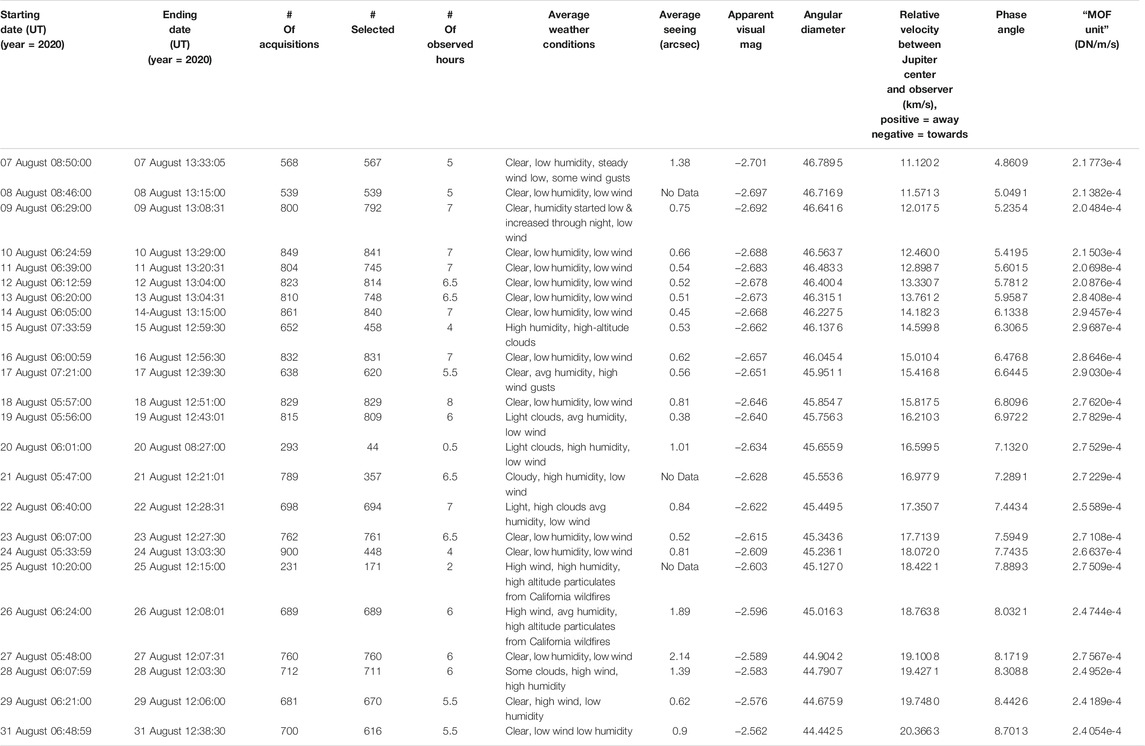
TABLE 1. Jovian observation statistics collected during the summer 2020 PMODE observational campaign on the AEOS 3.6 m telescope. Low humidity is defined as below 20%, high humidity is defined as greater than 60%. All statistics pertain directly to Jupiter, as other observed targets are not considered within this paper.

3.2 On-Sky Optimization

The transmission profile for each MOF is adjustable, with properties determined by both the choice of magnetic field (this is determined and fixed ahead of time within the surrounding permanent magnet assembly—for the K MOF, the magnetic field is fixed at 2 kG; for the Na MOF, the magnetic field is fixed at 3 kG) The second property which determines the MOF transmission profile is the (adjustable) temperature applied to the vapor cells. Increasing this temperature splits the passbands, increasing the area which is covered by the absorption line, but decreasing the steepness (which defines the sensitivity) of the absorption line profile. Additionally, applying a temperature which is too high can cause the vapor within the cell to deposit on the glass windows, resulting in failure of the cells. Therefore, finding the delicate balance between a temperature hot enough to provide sufficient surface coverage while maintaining a steep profile, and a temperature low enough that it will not damage the cell is necessary.

Determination of this temperature was conducted on-sky. We obtained frames of Jupiter through our finished system at varying temperature increments, in increasing steps of 2°C surrounding a predicted optimal temperature from previous simulations. For each collected data frame, we generated the corresponding Dopplergram and measured the contrast between the velocity band and the rest of the Jovian disk. The frame boasting the highest contrast between the two (and thus the highest sensitivity) corresponded to the optimal temperature. The contrast was determined by taking a horizontal cut through each Dopplergram to see the line profile across the disk, smoothing this profile to remove noise, then plotting the absolute value of the first derivative of this profile to determine which temperature had the highest values over the longest range. The same steps were repeated for the sodium channel: this calibration resulted in an optimal temperature determination of 89°C for the potassium channel, and an optimal temperature determination of 204°C for the sodium channel. This produces a single sharp line for potassium, with a smaller amount of disk coverage but higher sensitivity, and a split double line profile for sodium, resulting in a larger amount of disk coverage but shallower passbands with lower sensitivity. Combined, the two profiles provide high sensitivity and coverage over the majority of the Jovian disk (corresponding to the models shown in Figure 3).

4 Data Reduction Processes

4.1 Standard Calibrations

Data reduction was conducted with MATLAB to utilize its built-in image registration and signal processing routines. The developed pipelines include standard calibration techniques, sub-pixel image registration, field derotation, Jovian edge detection, background masking, and calculation (then subsequent subtraction of) a cleaned average frame. These reduction steps produce our final data product: a series of “residual images.” These final residual images are used to calculate the total integrated intensity, producing a time series for each channel of the instrumentation (although, as of yet, only the potassium data is considered due to the substantial detector noise in the sodium channel), within which we can begin the search for Jovian oscillations.

For a typical night of data processing, standard calibrations (bias-, dark-, “moon flat” (as detailed in Section 4.2) and bad pixel correction) are first applied to the full frame (consisting of both the MOF and continuum images), then a “leak image”—an average frame to account for any intensity leakage through our crossed polarizer and Wollaston, scaled to have a median value equal to the median value in the continnum frame—is subtracted from only the MOF side of the image. Therefore, to produce our final calibrated Dopplergram, the steps applied to the raw data are as follows:

$I_{Cal}=\frac{I_{Raw}-B-D}{F}(3)$

where I_Cal represents the calibrated intensity frame, I_Raw represents the raw intensity frame, B represents the median bias frame, D represents the median dark frame, and F represents the median “moon flat” frame. Following this standard reduction, the image is cropped so that the MOF image (V) and continuum image (C) are isolated. The leak image (L) is subtracted from V, which is then divided by C to produce the Dopplergram (DG), and subsequently divided by our MOF unit, VF (detailed in Section 2.2) for final amplitude calibration, as follows:

$DG=\frac{\left(V-L\right)}{C}\times \frac{1}{VF}(4)$

These calibration frames (biases, darks, and leak-images) were collected in bulk during the early nights of the observational campaign, and “quality check calibrations” were obtained periodically throughout the 24 days to ensure that the calibration frames were consistent and stable. Should any significant variations have appeared within the test calibration frames, the source of the difference would first be determined, then a second set of full calibration frames was planned to be corrected. However, these calibrations were stable over the course of the 24-day observational period, allowing our early-run calibrations to be utilized throughout the full dataset.

4.2 Moon Flats

It is important to note that our flat frames differ from the typical “in dome” evenly illuminated flat source (not present on the telescope the observations were conducted on), and also differ from typical sky-flats—indeed, the high sensitivity of the MOF technique requires a very brightly illuminated source, and neither dawn- nor twilight-sky frames provided the necessary photons within the MOF image on the detector. Instead, we decide to use portions of the Lunar surface as our flat field. Because the Lunar surface is not drastically moving towards or away from our observational location, Lunar observations provide a good zero point for velocimetric analysis. The extent of the Moon far overfills our field of view; thus, we are only able to observe a small portion of the surface at a time. To avoid any effects which could potentially be induced by observing only a specific regime, we requested that the telescope observers manually dither the observations via a “click and drag” method, coupled with simple drift scanning of the Lunar surface. This produced a dataset of constantly varying features, which average out when creating a “master flat.” We filled early-run down time between targets with these Moon flats when possible, collecting a total of 1,330 15-s exposure Moon flats spanning the date range from 08 August 2020 to 11 August 2020. Although each individual Lunar flat contains structural features (craters, maria, etc.), we are able to average these features out and produce a single flat-field image, thanks to the drift-scanning coupled with the click-and-drag method.

4.3 Image Registration

Although our MOF and continuum images move slightly within the field over the course of a night, there remains a standard, constant offset between these two images. This offset is known to better than 1/100th of a pixel, evidenced by our capability to fully cancel out albedo fluctuations and structure on the Jovian disk when the MOF image is divided by the (shifted) continuum image, producing a single Dopplergram (again, an image where the intensity in each pixel pertains to radial velocity towards or away from the observer, which must be multiplied by a scaling factor to translate intensity to velocity) for each frame. This Dopplergram is then derotated (to account for field rotation induced by the Alt-Az telescope) using the JPL Horizon ephemerides, then registered from frame-to-frame throughout the night. This registration is vitally important to avoid noise in our time series, so we apply a multi-step registration process. First, we use a zero-crossing Canny edge detection algorithm intrinsic to the MATLAB image registration toolbox. We chose to implement a zero-crossing edge detection technique because these techniques are insensitive to seeing-induced blurring, and have historically been successfully implemented in helioseismology (Toner and Jefferies (1993); Hill et al. (1975)). The Canny algorithm, in particular, was chosen for producing results similar to the classic Laplacian of a Gaussian registration technique, but with enhanced detection and localization performance (Canny, 1986).

Once this edge has been detected, we mask out the background surrounding the edge so that all that remains within the frame is the Dopplergram. Following this masking, we apply a monomodal intensity-based registration algorithm, also intrinsic to the MATLAB image registration toolbox, to register each Dopplergram to the exact center of the frame. The monomodal option was chosen in MATLAB because it is designed to work for images with similar intensity and contrast that collected on the same detector, and subsequently was well-suited for our registration attempts. This combination results in a frame-to-frame registration with an average error in stability which is smaller than 0.04 pixels. This monomodal intensity based registration is repeated once more within the data reduction process, following the Alt-Az derotation detailed in Section 4.6 to ensure that all velocigrams are truly in the direct center of each frame.

A median-combined average Dopplergram is then calculated from the co-registered Dopplergrams and subtracted from each to remove the effect of Jupiter’s rotation (as detailed further in Section 4.5), producing residual Dopplergrams. This average Dopplergram can be either a full combination of all frames throughout the night, or a “sliding average” of frames—for our project, we chose to utilize a sliding average over 200 frames (or 100 min), which effectively applies a high-pass smoothing filter of 166.67 μHz within the image domain. We chose this sliding average technique to reduce noise induced by seeing variations throughout the night, which increase towards the end of each night when Jupiter is observed through a higher airmass. These steps are visualized in Figure 6, specifically in Figures 6A–D.

FIGURE 6

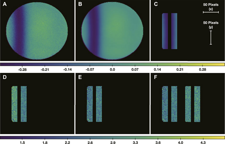
FIGURE 6. (A): a single Dopplergram, as seen in Figure 2C. (B): an average Dopplergram, created by median-combining all frames throughout the night. (C): the average Dopplergram, restricted to only the indices which are used in final calculation—the insensitive top, bottom, and central zones have been excluded, as well as all the disk outside the linear regime of the absorption line profile. (D): a single “residual image,” created by subtracting the average Dopplergram (Panel (C)) from the single Dopplergram (Panel (A)). (E): The left half of the residual image has been multiplied by a value of −1, to account for the change in sign when crossing the bottom of the absorption line. (F): the same steps are applied to a region opposite the center of the disk, in a region sufficiently outside the velocity-sensitive regime, to generate a “continuum residual” via the exact same process to characterize instrumental noise and effects. This panel shows the continuum residual plotted to the right of the velocity residual. Each row of panels maintains the same color scaling (corresponding to values of DN, or Data Numbers), as shown in the respective color bar below each trio. Each panel maintains the same axis scaling in pixels, as indicated by the inset bars in (C).

4.4 Additional Noise Sources

4.4.1 Tracking and Image Registration

Fine guiding for the PMODE observational campaign was done via a fast steering mirror operating at 0.5 KHz. It is presumed that these corrections, when integrated over a 30 s interval, do not significantly contribute noise to the signal. However, Jupiter’s position is only estimated via the limb finding routine—which we know to only be accurate to 1/20th of a pixel. These two errors are intrinsically combined and cannot be disentangled. This frame-to-frame image registration stability, with its error of approximately 0.04 pixels, provides a rough per-image noise level of 50 km s⁻¹ × 0.04 pix/200 pix = 10 m s⁻¹ approximately, which contributes to the total noise. This global error (induced from both tracking and registration) affects all pixels and is assumed to have no periodicity.

4.4.2 Distortion Noise

Unfortunately, no distortion calibration frames were collected during the observational campaign, rendering us unable to fully calibrate any distortion-induced noise. Our requirement during instrumentation build and calibration was to produce a distortion smaller than 1/10th of a pixel, and it is believed that this goal was achieved during alignment. Nonetheless, a distortion of this magnitude could still produce spurious effects on the velocity, which may be seen in the final images shown within Section 5.1.

4.4.3 Temperature Noise

The temperature of the cell was controlled to ±0.1 C. The experiment did not include logging of the temperature variation over time throughout the observational campaign, though quality-check routines were in place to alert the observers should temperatures exceed this acceptable variance of ±0.1 C. However, Cacciani et al. (2001) and Tomczyk et al. (1995) show that the error induced by temperature fluctuations on this level would be on order 10^–3 to 10^{–4 m} s⁻¹ in the frequency regime considered here. Therefore, we assume that noise induced by thermal fluctuations is significantly lower than other noise sources, and is not a particular point of concern.

4.5 Additional Velocity Calibrations

As we are searching for oscillation signals reportedly on the order of ∼50 cm s⁻¹ (Gaulme et al., 2011), it is necessary to perform a thorough and accurate calibration of the data to remove all additional velocities and potential noise sources. The observed Doppler shift of the reflected Solar K and Na lines are a combination of multiple different velocity sources, including: the relative motion between Jupiter and the Sun (V_J/⊙, which is uniform across the disk and manifests as a small and relatively constant offset of the center of the absorption line from the center of the Jovian disk on the order of tens of cm s⁻¹); the relative motion between the observer and Jupiter (encompassing both Earth’s rotation V_E,rot, which manifests as a predictable variation in intensity throughout a night, on the order of hundreds of m s⁻¹, and the Earth-Jupiter distance V_J/E, which is uniform across the disk and manifests as an offset in the center of the absorption line from the Jovian disk, on the order of a few km s⁻¹ and relatively constant throughout a single night but varying on a night-to-night basis); the Jovian rotation (V_J,rot which confines the sensitive region of the absorption line to a slice on the Jovian disk as detailed in Section 2.2, and is the only spatially defined additive velocity effect, manifesting as a variation of equatorial velocity from −12.57 to +12.57 km s⁻¹ across the Jovian disk from east to west); the Jovian smaller-scale atmospheric dynamics such as the zonal and meridional winds (V_J,Wind with velocities on the order of hundreds of m s⁻¹), and finally the oscillations themselves, V_Osc, expected to be on the order of ∼50 cm s⁻¹. The factor of (1 + cos(ϕ)) multiplying the summation of intrinsic Jovian-based factors, again, accounts for the doubling effect caused by reflection off of the Jovian atmosphere, where ϕ is the phase angle between Jupiter and Earth. A thorough detailing of these additive velocity effects is discussed in Gaulme et al. (2008), Gonçalves et al. (2019), and Cacciani et al. (2001). In summary, the entirety of the Doppler effects can be written as:

$V_{Doppler}=V_{J/\odot }+V_{E,rot}+V_{J/E}+\left(\left(1+\cos \left(\varphi \right)\right)\right)\left(V_{J,rot}+V_{J,Wind}+V_{Osc}\right)(5)$

Because these effects vary over long timescales, we remove them from our data simply by subtracting (from each frame) an average Dopplergram, consisting of the surrounding 200 registered and de-rotated Dopplergram frames, corresponding to an average over 100 min—this is effectively applying a moving, smoothing filter with a width of 166.67 μHz in the image domain. This value (200 frames) was chosen simply as an effective middle-ground between keeping the number of averages small enough to prevent any seeing-induced variations, but large enough to keep the smoothing filter relatively broad. This sliding filter is chosen to minimize seeing-induced differences which are apparent when subtracting only a single, nightly-average. Subtracting these average frames is beneficial in the search for the oscillations, which are expected to be long-lived, with significantly shorter periods than the subtracted 100-min average frame. We expect this subtraction to remove all additional Doppler effects without compromising any effects from the oscillations. By extension, to search for atmospheric dynamics via Doppler velocimetry, we examine these average image of each night to search for the zonal and meridional winds, as they are contained within it.

4.6 Alt-Az Derotation

As we were observing in the Coudé room of an Alt-Az telescope without a field derotation optic (a “K-mirror”), it was necessary to manually derotate the data frames so that the north pole of Jupiter was pointing north in our image frame. This was achieved using a JPL Horizons ephemerides which includes the timing information, altitude (alt), azimuth (az), declination (δ), hour angle (θ_H), and position angle (PA). With this data set and our site latitude (ϕ), we are then able to calculate the parallactic angle (θ_p) for each point in the epheremis, using Eq. 6, comprised of a Y defined by Eq. 7 and an X defined by Eq. 8. The factor of 15° multiplying the hour angle is included for a conversion to degrees.

${\theta }_p=atan2\left(Y,X\right)(6)$

where,

$Y=\mathit{sin}\left({\theta }_H\times 15°\right)(7)$

$X=\left(\mathit{tan}\left(\varphi \right)\times \mathit{cos}\left(\delta \right)\right)-\left(\mathit{sin}\left(\delta \right)\times \mathit{cos}\left({\theta }_H\times 15°\right)\right)(8)$

We then combine this calculated parallactic angle with the obtained position angle for Jupiter from the ephemerides to calculate the amount Jupiter (in our reference frame) needs to be rotated to point to our defined north in the image plane (we define this angle as θ_RN, for Rotate North):

${\theta }_{RN}=|{\theta }_p-az+alt-PA+C|(9)$

where the constant, C, defined the direction on our particular detector which we define as north. This constant is empirically determined to be +29.5°. This calculation generates an entire array matching the length of the ephemerides. We then find the closest time in this new array to the time which the image was obtained (in MJD), then rotate each of our images by its corresponding amount in the θ_RN array.

4.7 Dopplergram Cleaning and Spherical Harmonic Multiplication

The region outside the linear regime of the absorption line (which we define as the deepest 75% of the absorption line, excluding the ten pixels surrounding the very center of the line where sensitivity is low) is masked from each image. Next, we multiply the left half of the residual absorption line by a value of -1 to account for the change in sign when crossing the bottom of the absorption line, and then multiply these residual Dopplergram frames by the spherical harmonic of interest—for the sake of this paper, only the $Y_l^m$ = (0,0) and (1,0) harmonics, generated and fully normalized as follows:

$Y_{\ell }^m\left(\theta ,\varphi \right)=\frac{1}{\sqrt{2\pi }}{P}_{\ell }^m\left(\cos \theta \right)e^{im\varphi }(10)$

where $P_{\ell }^m(\cos \theta )$ represents the corresponding Legendre polynomial for a given ℓ and m, and the factor of $\frac{1}{\sqrt{2\pi }}$ is the normalization coefficient, chosen to ensure that the generated spherical harmonics are orthonormal over their full area (before restriction to the isolated regime on the Jovian disk), thereby preserving true amplitudes present within the dataset.

Finally, the intensity in each pixel of the residual velocigram (multiplied by the desired spherical harmonic) is integrated to produce a time series of Doppler data throughout each night. A description of this process for one single pixel is as follows:

$R=\left(DG-D{G}_{Avg}\right)\times Y_{\ell }^m\left(\theta ,\varphi \right)(11)$

where R represents residual intensity, DG represents a single Dopplergram, DG_Avg represents the average Dopplergram, and $Y_l^m(\theta ,\varphi )$ represents our desired, normalized spherical harmonic. This process is applied to each pixel in the image, and the resultant average of these final pixels is obtained as our final data product.

Finally, these same steps are applied to the right side of the Jovian disk, away from the absorption line, which can be seen in Figure 6E. Applying the exact same steps to an insensitive region of the disk allows us to utilize an in-image calibration source—because this side of the disk is outside the velocity sensitive regime of the absorption line, theoretically the values here should be a scaled constant, dependent on the intensities of the continuum and velocity frames. Any additional signal or variation in this constant can be attributed to instrumental or data processing noise, and is assumed to be present in both the continuum and velocity sides of the Dopplergram. A visualization of the Dopplergram at each step in the process from single image to final residual frames is shown in Figure 2.

4.8 Data Processing Pipeline Overview

A detailed list clarifying and summarizing each step carried out by the pipeline (and explained within the above sections) for the K MOF channel follows: 1) Rename each individual file by its corresponding MJD to easily keep track of timing. 2) Filter out spurious data from each night—data that has mean counts that are exceptionally low, or a variance that is exceptionally high. 3) Apply typical data reduction steps—bias, dark, and bad pixel correction. 4) Scale the leak image so that its median value is equal to the median value of the continuum frame, as the intensity of the leak image is proportional to the target intensity. Subtract this scaled leak image from the MOF image to account for crossed-polarizer leakage 5) Apply flat-field correction to the leak-corrected data frame. 6) Crop out the MOF image and the continuum image from each corrected data frame, based on the constant centers of the flat field. 7) Shift the continuum image to the MOF image, with sub-pixel image registration accuracy. 8) Once shifted, divide the MOF image by the continuum image to remove all Jovian disk structure and produce the Dopplergram. 9) Register the Dopplergram to the rough center of the frame (using a zero-crossing edge detection technique) for subsequent derotation. 10) Use the JPL Horizons ephemeris to derotate the data, to correct for observing on a Coudé Alt-Az telescope. 11) Detect the limb of the derotated Jupiter image using a zero-crossing approach, and mask out the background of the Dopplergram beyond this detected edge. 12) Shift each Dopplergram to be located in the center pixel of the image, so that the Dopplergrams are registered to the same location through the duration of the observing run. 13) Clean each Dopplergram so that only the deepest 75% of the absorption line profile remains, and the entirely of the disk outside of that region is removed. 14) Obtain the average Dopplergram for each night (either constant or a “sliding average” of 200 frames—100 min—166.67 μHz), depending on choice of analysis technique. For our final data products, we chose to utilize the sliding average technique to reduce noise), and subtract this from each individual Dopplergram to remove the Jovian rotation and produce residuals. 15) Multiply the left half of the residual by a value of −1 to account for the change in sign when crossing the bottom of the absorption line. 16) Multiply the residual image by the desired spherical harmonic. 17) Sum the intensity in the multiplied image, then normalize this by the number of pixels summed to get the residual intensity for the desired mode. Record this intensity along with the corresponding MJD for Fourier analysis. 18) Calculate the Lomb-Scargle periodigram of this data over the entirety of the observing run to obtain the power spectrum for the considered mode. 19) Apply these same techniques to the side of the Jovian disk with no velocity sensitivity to obtain a set of instrumental residuals. A visualization of these steps in their entirety, from first collected images on the detector to final residual images is shown within Figures 2, 6.

5 Preliminary Results

5.1 Jovian Zonal Winds

To validate our instrument design and confirm velocity sensitivity, we present spatially resolved Doppler measurements of the Jovian zonal winds. These winds are supposed to be low-contrast features with wind speeds ∼ 0.1% of the background signal coming from the Jovian rotation. In order to enhance the intricate structure of the Jovian zonal winds, a line-by-line high-pass filter is applied to nightly averages of the velocity-sensitive region of the disk. This method removes large-scale structure (such as a pedestal which is larger than the specified filter width) but can also be used as a tool to separate flows by wavenumber. As the dominating signal is assumed to be the Jovian rotation (which only varies on large spatial scales) and the zonal winds assumed to be small scale features, a band-pass filter can differentiate between the sources. The technique used is outlined in Reach et al. (1997); we summarize the process as applied to our data here. We begin by transforming the nightly averaged, PMODE derived velocigram into a planetographic coordinate system. Next, a Fourier transform is applied to the planetographic image to create $\mathcal{F}(I)$. We then create two maps that are representative of separate frequency regimes (Reach et al., 1997):

For the low-frequency signals:

$I_{\text{lf}}={\mathcal{F}}^{-1}\left[\mathcal{F}\left(I\right)e^{-f^2/2f_{\text{s}}^2}\right](12)$

To suppress high-frequency components in the original image we smooth via:

$I^{\prime }={\mathcal{F}}^{-1}\left[\mathcal{F}\left(I\right)\left(1-e^{-f^4/f_{\text{s}}^4}\right)\right](13)$

This allows us to separate frequency regimes by $f_{\text{lf}}^{-1}<\theta <f_{\text{s}}^{-1}$ as f is the spatial frequency projected on the disk. The final computation can be described using I_filtered = I′ − I_lf. The selection process to determine the quantities f_lf and f_s are described next. Zonal wind profiles can be decomposed into two separate regimes as defined by: a portion influenced by the all wavenumbers smaller than the wavenumber characterizing the large-scale friction (hereafter referred to as n_fr), and a portion containing all wavenumbers larger than n_fr. For Jupiter, Galperin et al. (2001) report a value of n_fr ≈ 20. Modes lower than n_fr are dominated by the equatorial jet, while modes higher than n_fr contain the remaining detailed structure. To focus on this smaller-scale structure of the winds, we choose a line-by-line high-pass filter commensurate with this wavenumber separating the two regimes. This process is visualized within Figure 7, which displays a Dopplergram before and after this filtering, and corresponding projections of the profile across the disk for both cases.

FIGURE 7

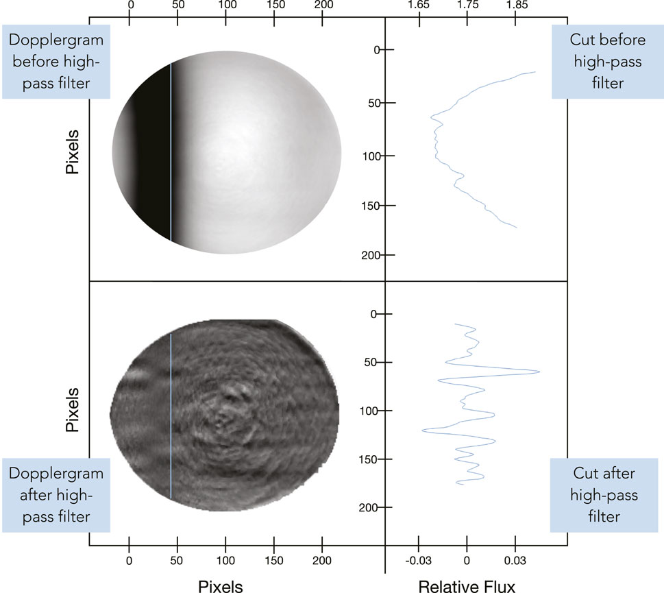
FIGURE 7. The top-left image shows a nightly-averaged Dopplergram before high-pass filtering. The top-right plot contains the projected information from the blue cut in the unfiltered image. The bottom-left images shows a nightly-averaged Dopplergram after high-pass filtering. The bottom-right plot contains the projected information from the blue cut in the filtered image. The images are displayed with the N-pole facing the top of the figure. Plots have been normalized and scaled—indicated by the axis labels.

The resultant profile after these calibrations is shown in Figure 8, where the profile is plotted as a black line with error bars displayed as the surrounding transparent grey region. Some geometrical distortion affects may be seen within this image: both the low frequency bias on the top image and spurious features in the center of the bottom image may be due to geometrical distortion, which remains for future analysis. This profile also contains information about the location of zone/belt interfaces that correspond with historical naming conventions, and shows three notable locations of increased variance:

FIGURE 8

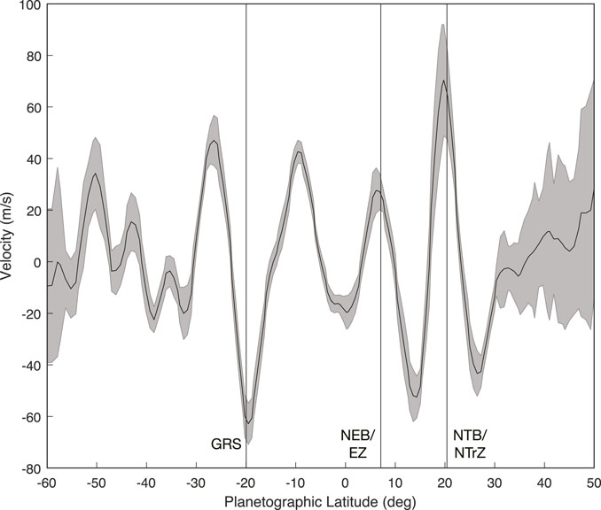
FIGURE 8. The average (high-pass filtered) Doppler velocimetric zonal wind profile of Jupiter derived from the 2020 observational campaign. The profile is plotted as a black line with error bars displayed as the surrounding transparent grey region. The locations of prominent region interfaces of interest (the GRS, NEB/EZ interface, and NTB/NTrZ interface) are marked with vertical lines. Positive velocity corresponds to the prograde direction and negative velocity corresponds to the retrograde direction.

The first location, at 22°S, is associated with the Great Red Spot (GRS), which is located between the Southern Equatorial Belt (SEB) and Southern Temperate Belt (STB). When the GRS is visible, we expect it to produce significant upwelling contributions. Due to the spatial aliasing associated with the instrument’s velocity-sensitive region, we expect a significant deviation from the mean—induced by a given night’s Jovicentric longitudinal coverage. Therefore, some nightly averages will include the GRS in the velocity-sensitive region, while others will not. That is to say, we expect a higher variation due to the inclusion (or lack thereof) of this region with enhanced upwelling. The second area of interest, at 7°N, is associated with the Northern Equatorial Belt (NEB) and Equatorial Zone (EZ) interface, and an increase in standard deviation may be explained as a result of plumes and hot spots in this region, which are theorized to be associated with a trapped planetary-scale equatorial Rossby wave. This region additionally manifests in the power series obtained from the K Doppler velocimetry channel, which is “contaminated” with signals that are likely partially related to these upwelling events in the region below 700 μHz (Lederer et al., 1995). The third area of interest, at 23°N, is associated with the interface between the Northern Temperate Belt (NTB) and Northern Tropical Zone (NTrZ).

The overall structure of the measured zonal wind velocity does bear a structural similarity with those acquired via cloud tracking methods (Barrado-Izagirre et al. (2013); Tollefson et al. (2017); Johnson et al. (2018)); however, the magnitude differs as a result of filtering out the low n_fr modes dominated by the equatorial jet. A future model-based approach, to include fine magnitude calibration, is necessary to adequately compare these results and their significance. We note that our zonal wind profile displays some differences to the sole previous Doppler velocimetric zonal wind measurements (Gonçalves et al., 2019). It is important to consider that these measurements were obtained at different times (5–6 years apart), and at a different wavelength (and thus, different atmospheric height), which could explain the discrepancy between the two measurements. Interestingly, the Gonçalves et al. (2019) zonal wind profile shows a similarity to the profile obtained when considering the low n_fr modes, while our results show a similarity to the profile derived for the high n_fr modes, both as compared to Galperin et al. (2001). It is certainly possible that a combination of these two separate Doppler velocimetric derived zonal wind profiles would accurately reproduce both the structure and amplitude derived via cloud tracking measurements, however, this is beyond the scope of this paper and remains for future analysis.

5.2 Sensitivity—Time Series Derived

While the lack of disk coverage can easily be seen as a detriment to any velocimetric analysis (e.g., in the case of significant spectral contamination via mode leakage), it does provide an inherent benefit to our calibration routine. A “null” region exists for much of the spatial extent of each Jupiter image. We can mirror a region about the disk center, by simply “flipping” our cleaned velocity region over the center of the disk so that it falls on an insensitive, continuum regime that then provides a separate portion of the Jovian disk to be used as a benchmark—this mirrored region can be seen directly beside the original continuum region within Figure 6E. This technique benefits from the ability to directly compare time series and spatially resolved signals that undergo identical processing steps, although the noise level in these two regimes differs purely due to a higher photon count in the insensitive regime as it falls outside of the projected absorption line on the Jovian disk.

Narrowing our search to compare with previous results, we first analyze the $Y_l^m=\left(\mathrm{0,0}\right)$ and $Y_l^m=\left(\mathrm{1,0}\right)$ spherical harmonic modes. The approach taken here assumes ideal scenarios and is only presented as a metric for instrument characterization. We apply a high-pass filter with a cutoff of 166 μHz (in the time-series domain) to reduce the effect of upwelling events occurring in active belts and zones that is present up to 700 μHz (Lederer et al., 1995)—our goal was not to fully eliminate these real upwelling signals, but to simply smooth a portion below this regime to minimize ringing and noise elsewhere in the spectrum (although certainly, it is not to be assumed that this low-frequency regime is solely due to Jovian origin. We expect some level of the low-frequency power to be attributed to instrumental noise, which remains to be analyzed and interpreted in its entirety within future work). To ensure that our amplitude-calibrated time series maintained its true amplitude through Fourier analysis, we included a conversion factor to retrieve amplitude from our Lomb-Scargle periodogram:

$A=\sqrt{\frac{2\times P\times f_s}{N_T}}(14)$

where A represents calibrated amplitude, P represents the resultant power from the Lomb-Scargle periodogram, f_s represents the frequency sampling rate (1/30 Hz), and N_T represents the number of samples in the true input time series.

To characterize the noise level of the background in our power spectra, we implemented a variety of techniques—first, we simply generated many (N is very large) permutated realizations of our time series and compute the Lomb-Scargle periodogram, producing a “noise spectrum” that we could then take a median value of to estimate the background level. This produced a value of around 16 cm s⁻¹ for the $Y_l^m=\left(\mathrm{1,0}\right)$ power spectrum. Selecting only a high-frequency regime and estimating the noise from this area produced a similar value. However, this noise certainly changes with frequency—thus, it is necessary to estimate the noise level specifically at the frequency range of interest. To do so, we first fit the background—however, this is not trivial, because a least square fitting is not appropriate for fitting a power spectrum since the distribution of a power spectrum is a chi square with 2 degrees of freedom. To compensate for this, we instead fit the average of many 2-day power spectra segments, similar to the process described in Appourchaux et al. (2014) and Gabriel et al. (2002) with a least square routine.

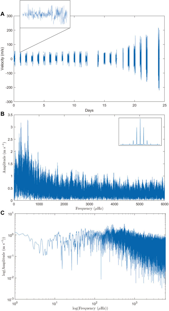
We now look to present the resultant preliminary amplitude spectra. As is expected, the $Y_l^m=\left(\mathrm{0,0}\right)$ mode—shown in Figure 9 (where Figure 9A displays the full time series of integrated intensity with a representative zoom-in, Figure 9B displays the calibrated amplitude spectrum with an inset window function in the upper right, and Figure 9C displays the same amplitude spectrum as Figure 9B, but with a log-log scaling)—contains a significantly higher noise-level due to a culmination of effects. The source of this noise includes contributions from atmospheric, instrumental, and pipeline effects (perhaps substantially affected by registration noise), all of which remain to be thoroughly analyzed and quantified in future work—these noise sources preference our analysis to the asymmetric mode, $Y_l^m=\left(\mathrm{1,0}\right)$. However, we do find it useful to describe the results of this Jupiter-as-a-star analysis. The power spectrum of the (0,0) mode in the “null” region has a standard deviation of 2 cm s⁻¹. This demonstrates the quality of the calibration and the pipeline routine. However, it is important to note that, because the null region is unaffected by the absorption line profile, it also has a higher flux (nearly by a factor of 2 once in “Dopplergram space”, and therefore, maintains a lower signal-to-noise ratio) than our velocity sensitive regime. Moving forward, with this information, we expect that albedo fluctuations are unlikely capable of producing significant signals in our data. For the velocity sensitive regime of the $Y_l^m=\left(\mathrm{0,0}\right)$ data (as opposed to the null regime), the background fitting routine displays a noise level of less than 1.05 m s⁻¹ in the regime beyond 800 μHz.

FIGURE 9

FIGURE 9. (A): $Y_l^m=\left(\mathrm{0,0}\right)$ time series for the full 24-day observational campaign. A representative night is shown in an inset for ease of interpretation. (B): Preliminary $Y_l^m=\left(\mathrm{0,0}\right)$ calibrated amplitude spectrum for the full 24-day observational campaign. The window function is shown as an inset in the upper right-hand corner of this panel. (C): Preliminary $Y_l^m=\left(\mathrm{0,0}\right)$ amplitude spectrum, as in Panel (B), in a log-log scale.

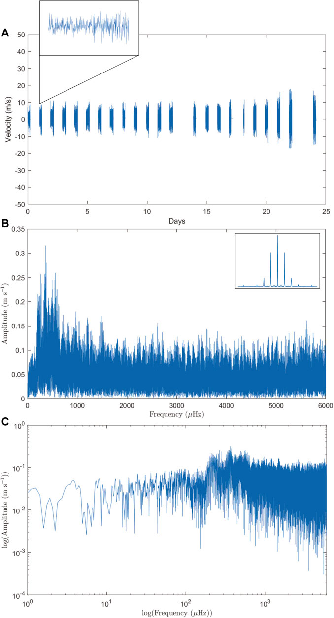
The asymmetric mode—$Y_l^m=\left(\mathrm{1,0}\right)$ is shown in Figure 10 (where Figure 10A displays the full time series of integrated intensity with a representative zoom-in, Figure 10B displays the calibrated amplitude spectrum with an inset window function in the upper right, and Figure 10C displays the same amplitude spectrum). The net cancellation of globally present signals on a given Dopplergram reduces the noise in our time series analysis considerably. Although a noise reduction was expected from application of an antisymmetric mask, we acknowledge that the drastic noise level difference between the $Y_l^m=\left(\mathrm{0,0}\right)$ and $Y_l^m=\left(\mathrm{1,0}\right)$ modes is certainly surprising and requires a deeper examination in future work, which is beyond the scope of this paper. This amplitude spectrum, along with our aforementioned background fitting provides a noise level of lower than 16 cm s⁻¹ in the entire regime beyond 800 μHz for the $Y_l^m=\left(\mathrm{1,0}\right)$ mode, and a minimum noise level of 13 cm s⁻¹ at 1,200 μHz.

FIGURE 10

FIGURE 10. (A): $Y_l^m=\left(\mathrm{1,0}\right)$ time series for the full 24-day observational campaign. A representative night is shown in an inset for ease of interpretation. (B): Preliminary $Y_l^m=\left(\mathrm{1,0}\right)$ calibrated amplitude spectrum for the full 24-day observational campaign. The window function is shown as an inset in the upper right-hand corner of this panel. (C): Preliminary $Y_l^m=\left(\mathrm{1,0}\right)$ amplitude spectrum, as in (B), in a log-log scale.

These data, when analyzed in further detail, can provide information on the expected excitation mechanisms and place constraints on the maximum possible amplitudes for the global modes of Jupiter. Currently, models are unable to reproduce mode amplitudes that exceed the limits constrained by our sensitivity limit (Markham and Stevenson, 2018). The sole exception to this is in the case of excitation by rock-storms; the existence of which is yet to be confirmed for Jupiter.

6 Conclusion

To further constrain the atmospheric dynamics at play on Jupiter, we conducted a 24-day observational campaign on the AEOS 3.6 m telescope during the summer of 2020 with PMODE. This multi-channel instrument, which includes a Doppler velocimeter, achieved sub-arcsecond resolution. Here, we present first results from the potassium Doppler imager channel of this experiment in the form of an independent Doppler measurement of the zonal wind profile in the upper troposphere. We compare our results with previous measurements to determine that this profile shows structural similarities to zonal wind profiles collected through cloud-tracking measurements, and similarity in both structure and amplitude to the zonal wind profile that is derived from Voyager measurements (Galperin et al., 2001) when isolating the components to only those unaffected by the equatorial jet. When combined with previous Doppler measurements of the zonal wind profile which show a similarity to the zonal wind profile containing the equatorial jet regime (Gonçalves et al., 2019), we expect that Doppler measurements of the zonal wind profile may reproduce—in both structure and amplitude—a profile matching those obtained from feature-tracking techniques; this combination of profiles is ongoing. Current preliminary analysis of our amplitude spectra for low-order modes displays no significant, organized power in the region of interest (1,100–1,200 μHz) with amplitudes greater than our noise floor of 16 cm s⁻¹. A future refined analysis of this dataset will place strict upper limits on the maximum amplitude for the global modes of Jupiter, will provide an avenue to constrain excitation mechanisms, and will also allow for discussion of temporal variability of the zonal winds over a consecutive 24-day time frame.

Data Availability Statement

The raw data supporting the conclusion of this article will be made available by the authors, without undue reservation.

Author Contributions

CS: Designed/built/aligned the instrumentation, simulated expected results, conducted the observations, prepared the figures, analyzed and interpreted the data, and wrote and edited the manuscript. DG: Simulated expected results, conducted the observations, prepared the figures, analyzed and interpreted the data, and wrote and edited the manuscript. RS: Designed the instrumentation, conceived the project, provided observational assistance, wrote and edited the manuscript. SJ: Provided observational assistance, supervised the study, and analyzed and interpreted the data. NM: Designed and constructed the vapor cells, provided observational assistance, supervised the study, analyzed and interpreted the data, and edited the manuscript.

Funding

The Air Force Office of Scientific Research funded this work through contracts FA9451-20-F-0004 TO2 (CS). This material is based upon work supported by the National Science Foundation Graduate Research Fellowship under Grant No. 1937956 (DG). This research was supported by the Jet Propulsion Laboratory, California Institute of Technology, under contract with the National Aeronautics and Space Administration (NM). SMJ and DJG were funded by FA9451-19-2-0035.

Conflict of Interest

Author RS was employed by the company Odyssey Systems.

The remaining authors declare that the research was conducted in the absence of any commercial or financial relationships that could be construed as a potential conflict of interest.

Publisher’s Note

All claims expressed in this article are solely those of the authors and do not necessarily represent those of their affiliated organizations, or those of the publisher, the editors and the reviewers. Any product that may be evaluated in this article, or claim that may be made by its manufacturer, is not guaranteed or endorsed by the publisher.

Acknowledgments

The authors would like to extend their sincere and deep appreciation to Jason Jackiewicz for his significant contribution and assistance in amplitude calibration for the frequency-domain analysis. We thank Raúl Morales-Juberías for his input and discussion on interpretation of the PMODE zonal wind measurement. We acknowledge and greatly appreciate the support from various staff members at the observatory from which this data was collected: Chris Shurilla, Ryan Conway, and Shadi Naderi. The observers from the summer 2020 campaign: Lanz, Dianna, Tyler, Chaz, Kalen, Theresa, and Mo. We would also like to thank the reviewers for their insightful comments and dedicated efforts towards improving our manuscript.

References

Agnelli, G., Cacciani, A., and Fofi, M. (1975). The Magneto-Optical Filter. Sol. Phys. 44, 509–518. doi:10.1007/BF00153229

CrossRef Full Text | Google Scholar

Appourchaux, T., Antia, H. M., Benomar, O., Campante, T. L., Davies, G. R., Handberg, R., et al. (2014). Oscillation Mode Linewidths and Heights of 23 Main-Sequence Stars Observed byKepler. Astron. Astrophys. 566, A20. doi:10.1051/0004-6361/201323317

CrossRef Full Text | Google Scholar

Arregi, J., Rojas, J. F., Sánchez-Lavega, A., and Morgado, A. (2006). Phase Dispersion Relation of the 5-micron Hot Spot Wave from a Long-Term Study of jupiter in the Visible. J. Geophys. Res. 111, 7–9. doi:10.1029/2005JE002653

CrossRef Full Text | Google Scholar

Barrado-Izagirre, N., Rojas, J. F., Hueso, R., Sánchez-Lavega, A., Colas, F., Dauvergne, J. L., et al. (2013). Jupiter's Zonal Winds and Their Variability Studied with Small-Size Telescopes. Astron. Astrophys. 554, A74. doi:10.1051/0004-6361/201321201

CrossRef Full Text | Google Scholar

Brogi, M., Kok, R. J. d., Albert, S., Snellen, I. A. G., Birkby, J. L., Schwarz, H., et al. (2016). Rotation and Winds of Exoplanet Hd 189733 B Measured with High-Dispersion Transmission Spectroscopy. ApJ 817, 106. doi:10.3847/0004-637X/817/2/106

CrossRef Full Text | Google Scholar

Cacciani, A., Dolci, M., Giuliani, C., and Moretti, P. (1998). “A Jupiter Seismology Project,” in Structure and Dynamics of the Interior of the Sun and Sun-like Stars. ESA Special Publication, 418, 381.

Google Scholar

Cacciani, A., Dolci, M., Moretti, P. F., D'Alessio, F., Giuliani, C., Micolucci, E., et al. (2001). Search for Global Oscillations on Jupiter with a Double-Cell Sodium Magneto-Optical Filter. Astron. Astrophys. 372, 317–325. Number: 1 Publisher: EDP Sciences. doi:10.1051/0004-6361:20010455

CrossRef Full Text | Google Scholar

Cacciani, A., and Fofi, M. (1978). The Magneto-Optical Filter. Sol. Phys. 59, 179–189. doi:10.1007/BF00154941

CrossRef Full Text | Google Scholar

Canny, J. (1986). “A Computational Approach to Edge Detection,” in IEEE Transactions on Pattern Analysis and Machine Intelligence, PAMI-8, 679–698. doi:10.1109/TPAMI.1986.4767851

CrossRef Full Text | Google Scholar

Civeit, T., Appourchaux, T., Lebreton, J.-P., Luz, D., Courtin, R., Neiner, C., et al. (2005). On Measuring Planetary Winds Using High-Resolution Spectroscopy in Visible Wavelengths. Astron. Astrophys. 431, 1157–1166. doi:10.1051/0004-6361:20041640

CrossRef Full Text | Google Scholar

Dick, D. J., and Shay, T. M. (1991). Ultrahigh-Noise Rejection Optical Filter. Opt. Lett. 16, 867–869. doi:10.1364/OL.16.000867

PubMed Abstract | CrossRef Full Text | Google Scholar

Dowling, T. E. (1995). Dynamics of Jovian Atmospheres. Annu. Rev. Fluid Mech. 27, 293–334. doi:10.1146/annurev.fl.27.010195.001453

CrossRef Full Text | Google Scholar

Fletcher, L. N., Greathouse, T. K., Orton, G. S., Sinclair, J. A., Giles, R. S., Irwin, P. G. J., et al. (2016). Mid-infrared Mapping of jupiter’s Temperatures, Aerosol Opacity and Chemical Distributions with Irtf/texes. Icarus 278, 128–161. doi:10.1016/j.icarus.2016.06.008

CrossRef Full Text | Google Scholar

Fletcher, L. N., Helled, R., Roussos, E., Jones, G., Charnoz, S., André, N., et al. (2020a). Ice Giant Systems: The Scientific Potential of Orbital Missions to Uranus and neptune. Planet. Space Sci. 191, 105030. doi:10.1016/j.pss.2020.105030

CrossRef Full Text | Google Scholar

Fletcher, L. N., Kaspi, Y., Guillot, T., and Showman, A. P. (2020b). How Well Do We Understand the belt/zone Circulation of Giant Planet Atmospheres? Space Sci. Rev. 216, 30. doi:10.1007/s11214-019-0631-9

PubMed Abstract | CrossRef Full Text | Google Scholar

Gabriel, A. H., Baudin, F., Boumier, P., García, R. A., Turck-Chièze, S., Appourchaux, T., et al. (2002). A Search for Solar $\vec{g}$ Modes in the GOLF Data. Astron. Astrophys. 390, 1119–1131. doi:10.1051/0004-6361:20020695

CrossRef Full Text | Google Scholar

Galperin, B., Sukoriansky, S., and Huang, H.-P. (2001). Universal N−5 Spectrum of Zonal Flows on Giant Planets. Phys. Fluids 13, 1545–1548. doi:10.1063/1.1373684

CrossRef Full Text | Google Scholar

Gaulme, P., Schmider, F. X., Gay, J., Jacob, C., Alvarez, M., Reyes-Ruiz, M., et al. (2008). SYMPA, a Dedicated Instrument for Jovian Seismology. II. Real Performance and First Results. Astron. Astrophys. 490, 859–871. ArXiv: 0802.1777. doi:10.1051/0004-6361:200809512

CrossRef Full Text | Google Scholar

Gaulme, P., Schmider, F.-X., Gay, J., Guillot, T., and Jacob, C. (2011). Detection of Jovian Seismic Waves: a New Probe of its interior Structure. Astron. Astrophys. 531, A104. doi:10.1051/0004-6361/201116903

CrossRef Full Text | Google Scholar

Gaulme, P., Schmider, F.-X., and Gonçalves, I. (2018). Measuring Planetary Atmospheric Dynamics with Doppler Spectroscopy. Astron. Astrophys. 617, A41. doi:10.1051/0004-6361/201832868

CrossRef Full Text | Google Scholar

Gaulme, P., Schmider, F.-X., Widemann, T., Gonçalves, I., López Ariste, A., and Gelly, B. (2019). Atmospheric Circulation of Venus Measured with Visible Imaging Spectroscopy at the THEMIS Observatory. Astron. Astrophys. 627, A82. doi:10.1051/0004-6361/201833627

CrossRef Full Text | Google Scholar

Gonçalves, I., Schmider, F. X., Gaulme, P., Morales-Juberías, R., Guillot, T., Rivet, J.-P., et al. (2019). First Measurements of Jupiter's Zonal Winds with Visible Imaging Spectroscopy. Icarus 319, 795–811. doi:10.1016/j.icarus.2018.10.019

CrossRef Full Text | Google Scholar

Guillot, T. (2005). THE INTERIORS OF GIANT PLANETS: Models and Outstanding Questions. Annu. Rev. Earth Planet. Sci. 33, 493–530. doi:10.1146/annurev.earth.32.101802.120325

CrossRef Full Text | Google Scholar

Helled, R., Anderson, J. D., Podolak, M., and Schubert, G. (2010). Interior Models of Uranus and neptune. ApJ 726, 15. doi:10.1088/0004-637x/726/1/15

CrossRef Full Text | Google Scholar

Hill, H. A., Stebbins, R. T., and Oleson, J. R. (1975). The Finite Fourier Transform Definition of an Edge on the Solar Disk. ApJ 200, 484–498. ADS Bibcode: 1975ApJ…200\enleadertwodots 484H. doi:10.1086/153814

CrossRef Full Text | Google Scholar

Hubbard, W. B. (1999). Gravitational Signature of Jupiter's Deep Zonal Flows. Icarus 137, 357–359. doi:10.1006/icar.1998.6064

CrossRef Full Text | Google Scholar

Ingersoll, A. P., and Pollard, D. (1982). Motion in the Interiors and Atmospheres of jupiter and Saturn: Scale Analysis, Anelastic Equations, Barotropic Stability Criterion. Icarus 52, 62–80. doi:10.1016/0019-1035(82)90169-5

CrossRef Full Text | Google Scholar

Ingersoll, A. P., Dowling, T. E., Gierasch, P. J., Orton, G. S., Read, P. L., Sánchez-Lavega, A., et al. (2004). “Dynamics of Jupiter’s Atmosphere,” in Jupiter: The Planet, Satellites, and Magnetosphere (Cambridge: Cambridge University Press), Vol. 1, 105–128.

Google Scholar

Johnson, P. E., Morales-Juberías, R., Simon, A., Gaulme, P., Wong, M. H., and Cosentino, R. G. (2018). Longitudinal Variability in Jupiter's Zonal Winds Derived from Multi-Wavelength HST Observations. Planet. Space Sci. 155, 2–11. doi:10.1016/j.pss.2018.01.004

CrossRef Full Text | Google Scholar

Kaspi, Y., Galanti, E., Hubbard, W. B., Stevenson, D. J., Bolton, S. J., Iess, L., et al. (2018). Jupiter's Atmospheric Jet Streams Extend Thousands of Kilometres Deep. Nature 555, 223–226. doi:10.1038/nature25793

PubMed Abstract | CrossRef Full Text | Google Scholar

Kong, D., Zhang, K., Schubert, G., and Anderson, J. D. (2018). Origin of Jupiter's Cloud-Level Zonal Winds Remains a Puzzle Even after Juno. Proc. Natl. Acad. Sci. USA 115, 8499–8504. doi:10.1073/pnas.1805927115

PubMed Abstract | CrossRef Full Text | Google Scholar

Lederer, S. M., Marley, M. S., Mosser, B., Maillard, J. P., Chanover, N. J., and Beebe, R. F. (1995). Albedo Features and Jovian Seismology. Icarus 114, 269–277. doi:10.1006/icar.1995.1061

CrossRef Full Text | Google Scholar

Lellouch, E., and Witasse, O. (2008). A Coordinated Campaign of Venus Ground-Based Observations and Venus Express Measurements. Planet. Space Sci. 56, 1317–1319. doi:10.1016/j.pss.2008.07.001

CrossRef Full Text | Google Scholar

Lellouch, E., Goldstein, J. J., Rosenqvist, J., Bougher, S. W., and Paubert, G. (1994). Global Circulation, Thermal Structure, and Carbon Monoxide Distribution in Venus' Mesosphere in 1991. Icarus 110, 315–339. doi:10.1006/icar.1994.1125

CrossRef Full Text | Google Scholar

Liu, S.-F., Hori, Y., Müller, S., Zheng, X., Helled, R., Lin, D., et al. (2019). The Formation of Jupiter's Diluted Core by a Giant Impact. Nature 572, 355–357. doi:10.1038/s41586-019-1470-2

PubMed Abstract | CrossRef Full Text | Google Scholar

Louden, T., and Wheatley, P. J. (2015). Spatially Resolved Eastward Winds and Rotation of Hd 189733b. Astrophysical J. Lett. 814, 3–4. doi:10.1088/2041-8205/814/2/l24

CrossRef Full Text | Google Scholar

Luz, D., Civeit, T., Courtin, R., Lebreton, J., Gautier, D., Rannou, P., et al. (2005). Characterization of Zonal Winds in the Stratosphere of Titan with UVES. Icarus 179, 497–510. doi:10.1016/j.icarus.2005.07.021

CrossRef Full Text | Google Scholar

Luz, D., Civeit, T., Courtin, R., Lebreton, J.-P., Gautier, D., Witasse, O., et al. (2006). Characterization of Zonal Winds in the Stratosphere of Titan with UVES: 2. Observations Coordinated with the Huygens Probe Entry. J. Geophys. Res. 111, E08S90. doi:10.1029/2005JE002617

CrossRef Full Text | Google Scholar

Machado, P., Luz, D., Widemann, T., Lellouch, E., and Witasse, O. (2012). Mapping Zonal Winds at Venus's Cloud Tops from Ground-Based Doppler Velocimetry. Icarus 221, 248–261. doi:10.1016/j.icarus.2012.07.012

CrossRef Full Text | Google Scholar

Machado, P., Widemann, T., Peralta, J., Gonçalves, R., Donati, J.-F., and Luz, D. (2017). Venus Cloud-Tracked and Doppler Velocimetry Winds from CFHT/ESPaDOnS and Venus Express/VIRTIS in April 2014. Icarus 285, 8–26. doi:10.1016/j.icarus.2016.12.017

CrossRef Full Text | Google Scholar

Markham, S., and Stevenson, D. (2018). Excitation Mechanisms for Jovian Seismic Modes. Icarus 306, 200–213. doi:10.1016/j.icarus.2018.02.015

CrossRef Full Text | Google Scholar

Mosser, B., Mekarnia, D., Maillard, J. P., Gay, J., Gautier, D., and Delache, P. (1993). Seismological Observations with a Fourier Transform Spectrometer - Detection of Jovian Oscillations. Astron. Astrophys. 267, 604–622.

Google Scholar

Mosser, B., Maillard, J. P., and Mékarnia, D. (2000). New Attempt at Detecting the Jovian Oscillations. Icarus 144, 104–113. doi:10.1006/icar.1999.6271

CrossRef Full Text | Google Scholar

Reach, W. T., Franz, B. A., and Weiland, J. L. (1997). The Three-Dimensional Structure of the Zodiacal Dust Bands. Icarus 127, 461–484. doi:10.1006/icar.1997.5704

CrossRef Full Text | Google Scholar

Roberts, L. C., and Neyman, C. R. (2002). Characterization of the AEOS Adaptive Optics System. Publ. Astron. Soc. Pac. 114, 1260–1266. doi:10.1086/343221

CrossRef Full Text | Google Scholar

Sánchez-Lavega, A., Rogers, J. H., Orton, G. S., García-Melendo, E., Legarreta, J., Colas, F., et al. (2017). A Planetary-Scale Disturbance in the Most Intense Jovian Atmospheric Jet from Junocam and Ground-Based Observations. Geophys. Res. Lett. 44, 4679–4686. doi:10.1002/2017GL073421

CrossRef Full Text | Google Scholar

Schmider, F.-X., Fossat, E., and Mosser, B. (1991). Possible Detection of Jovian Global Oscillations. Astron. Astrophys. 248, 281–291.

Google Scholar

Schmider, F. X., Gay, J., Gaulme, P., Jacob, C., Abe, L., Alvarez, M., et al. (2007). SYMPA, a Dedicated Instrument for Jovian Seismology. I. Principle and Performance. Astron. Astrophys. 474, 1073–1080. doi:10.1051/0004-6361:20067019

CrossRef Full Text | Google Scholar

Showman, A. P., and Dowling, T. E. (2000). Nonlinear Simulations of Jupiter's 5-Micron Hot Spots. Science 289, 1737–1740. doi:10.1126/science.289.5485.1737

PubMed Abstract | CrossRef Full Text | Google Scholar

Simon, M. C. (1986). Wollaston Prism with Large Split Angle. Appl. Opt. 25, 369–376. doi:10.1364/AO.25.000369

PubMed Abstract | CrossRef Full Text | Google Scholar

Stevenson, D. J. (2020). Jupiter's Interior as Revealed by Juno. Annu. Rev. Earth Planet. Sci. 48, 465–489. doi:10.1146/annurev-earth-081619-052855

CrossRef Full Text | Google Scholar

Tollefson, J., Wong, M. H., Pater, I. d., Simon, A. A., Orton, G. S., Rogers, J. H., et al. (2017). Changes in Jupiter's Zonal Wind Profile Preceding and during the Juno mission. Icarus 296, 163–178. doi:10.1016/j.icarus.2017.06.007

CrossRef Full Text | Google Scholar

Tomczyk, S., Streander, K., Card, G., Elmore, D., Hull, H., and Cacciani, A. (1995). An Instrument to Observe Low-Degree Solar Oscillations. Sol. Phys. 159, 1–21. doi:10.1007/BF00733027

CrossRef Full Text | Google Scholar

Toner, C. G., and Jefferies, S. M. (1993). Accurate Measurement of the Geometry for a Full-Disk Solar Image and Estimation of the Observational point Spread Function. ApJ 415, 852. doi:10.1086/173207

CrossRef Full Text | Google Scholar

Vorontsov, S. V., Zharkov, V. N., and Lubimov, V. M. (1976). The Free Oscillations of jupiter and Saturn. Icarus 27, 109–118. doi:10.1016/0019-1035(76)90187-1

CrossRef Full Text | Google Scholar

Wahl, S. M., Hubbard, W. B., Militzer, B., Guillot, T., Miguel, Y., Movshovitz, N., et al. (2017). Comparing jupiter interior Structure Models to Juno Gravity Measurements and the Role of a Dilute Core. Geophys. Res. Lett. 44, 4649–4659. ArXiv: 1707.01997. doi:10.1002/2017GL073160

CrossRef Full Text | Google Scholar

West, R. A., Baines, K. H., Friedson, A. J., Banfield, D., Ragent, B., and Taylor, F. W. (2004). “Jovian Clouds and Haze,” in Jupiter: The Planet, Satellites and Magnetosphere, 79–104. 9780521818087.

Google Scholar

Widemann, T., Lellouch, E., and Donati, J.-F. (2008). Venus Doppler Winds at Cloud Tops Observed with ESPaDOnS at CFHT. Planet. Space Sci. 56, 1320–1334. doi:10.1016/j.pss.2008.07.005

CrossRef Full Text | Google Scholar