The Lambert-Topp-Leone distribution: an alternative for modeling proportion and lifetime data

This article discusses the Lambert-Topp-Leone distribution as a flexible alternative for modeling proportion and lifetime data. By extending the Topp-Leone distribution, the proposed model offers greater flexibility in terms of skewness and kurtosis, making it suitable for a broader range of real-world applications. We examine key properties of the distribution, including its moments and behavior in terms of skewness and kurtosis. Parameter estimation using the maximum likelihood method is also discussed. A Monte Carlo simulation study is conducted to evaluate the performance of the estimators. Finally, to illustrate its practical utility, we apply the Lambert-Topp-Leone distribution to real-world datasets, demonstrating its superior fit for proportion and lifetime data compared to traditional models. The results suggest that this distribution provides a valuable tool for researchers and professionals in fields that require versatile modeling of bounded or positively skewed data.

1 Introduction

The Topp-Leone (TL) distribution is a continuous probability distribution often used to model bounded data, especially when a decreasing or unimodal pattern in the frequency of events is observed. It was originally proposed by Topp and Leone [1] as an alternative for modeling failure data. The cumulative distribution function (CDF), the probability density function (PDF), and the quantile function (QF) of the TL distribution are expressed as follows:

$\begin{array}{ll}F(x)={(1-y^2)}^{\beta },& (1)\end{array}$

$\begin{array}{ll}f(x)=\frac{2\beta }{b}y{(1-y^2)}^{\beta -1}\text{and}& (2)\end{array}$

$\begin{array}{ll}{F}^{-1}(u)=b\left(1-\sqrt{1-u^{\frac{1}{\beta }}}\right),& (3)\end{array}$

respectively, where y = 1 − x/b, 0 < x < b, b > 0, 0 < u < 1, and 0 < β < 1.

Topp and Leone [1] impose the restriction 0 < β < 1 because their goal was to study a distribution with a J-shaped probability density function. Specifically, they were interested in the case where f(x) > 0, f′(x) < 0 and f″(x) > 0 for all 0 < x < b, where f′ and f″ are the first and second derivatives of Equation 2, respectively. Currently, studies involving the TL distribution consider b > 0, so Equation 2 has a unimodal shape when b > 1.

The TL distribution has been studied by various authors. Nadarajah and Kotz [2] derive closed-form analytical expressions for the hazard rate function and moments of this distribution. For example, Ghitany et al. [3] study reliability measures of the TL distribution. Zhou et al. [4] study the distribution of the sum, product, and quotients of TL random variables. Kotz and Seier [5] explore the kurtosis behavior of the TL distribution by using the spread-spread function. Nadarajah [6] studies different distributions with a bathtub hazard rate function, including the TL distribution. Genç [7] studies the moments of the order statistics of the TL distribution.

The TL distribution's analytical simplicity and shape flexibility (J-shaped and unimodal) make it a valuable alternative for fitting bounded data. However, there are occasions when the data exhibit high levels of skewness and kurtosis, which can impair the performance of this distribution in fitting the data. In the literature, various approaches can be found to introduce one or more parameters to an arbitrary baseline distribution, which results in greater flexibility in terms of skewness and kurtosis. See, for example [8–15].

In this context, Iriarte et al. [16] propose the Lambert-F distribution generator, whose CDF is defined by

$\begin{array}{ll}G(x;\alpha ,\eta )=1-\left[1-F(x;\eta )\right]{\alpha }^{F(x;\eta )},& (4)\end{array}$

where F(·;η) is the CDF of an arbitrary baseline distribution with parameter vector η, α ∈ (0, e) is an extra shape parameter, and e ≈ 2.718 is the Euler's number.

The corresponding PDF and QF are given by

$\begin{array}{ll}g(x;\alpha ,\eta )=f(x;\eta ){\alpha }^{F(x;\eta )}\left\{1-log(\alpha )\left[1-F(x;\eta )\right]\right\}\text{and}& (5)\end{array}$

$\begin{array}{ll}{G}^{-1}(p;\alpha ,\eta )=\{\begin{array}{l}{F}^{-1}\left(\frac{W_0\left(\frac{\log (\alpha )(p-1)}{\alpha }\right)}{\log (\alpha )};\eta \right),\text{ if }\alpha \ne 1,\hfill \\ F^{-1}(p),\text{ if }\alpha =1,\hfill \end{array}& (6)\end{array}$

respectively, where p ∈ (0, 1), F(·;η), F⁻¹(·;η), and f(·;η) are the CDF, the QF, and the PDF of the baseline distribution, and W₀(·) is the principal branch of the Lambert W function.

Lambert-F distributions exhibit wider ranges of skewness than the corresponding baseline distributions, making them an important alternative for modeling skewed data. See, for example [17–19].

This study presents a new distribution for bounded data, the Lambert-Topp-Leone (LTL) distribution. It arises by considering a baseline TL distribution in the Lambert-F distribution generator. In consequence, an extension of the TL distribution that includes an additional shape parameter, offering more flexibility in terms of skewness and kurtosis, is defined. The new distribution can serve as an alternative to the beta [20] and Kumaraswamy [21] distributions, or to recently introduced distributions such as the NXLD [22], which are widely used for analyzing proportion data. In the context of lifetime data analysis, this distribution can serve as an alternative to the Weibull [23], Birnbaum-Saunders [24], generalized exponential [25], and generalized Rayleigh [26] distributions.

The rest of the article is organized as follows: In Section 2, the new distribution is introduced, its behavior in terms of skewness and kurtosis is described, and the hazard rate function is analyzed. Section 3 discusses parameter estimation using the maximum likelihood method and presents a simulation study to evaluate the performance of the estimators. Section 4 presents several real-world applications, including proportion data on household spending allocated to food and lifetime data on fatigue. These applications demonstrate that the new distribution may provide a better fit to the data compared to traditional distributions. Finally, concluding remarks are presented in Section 6.

2 The new distribution

In this section, we introduce the Lambert-Topp-Leone (LTL) random variable and study some of its main properties.

2.1 The Lambert-Topp-Leone random variable

In this section, we introduce the LTL random variable and present its PDF, CDF, and QF.

Proposition 1. A random variable X follows the Lambert-Topp-Leone (LTL) distribution, with parameters α ∈ (0, e) and β, b > 0, denoted as X ~ LTL(α, β, b), if its CDF, QF, and PDF are given, respectively, by

$\begin{array}{ll}G(x;\alpha ,\beta ,b)=1-\left[1-{(1-y^2)}^{\beta }\right]{\alpha }^{{(1-y^2)}^{\beta }},& (7)\end{array}$

$\begin{array}{ll}{G}^{-1}(p;\alpha ,\beta ,b)=\{\begin{array}{l}b\left[1-\sqrt{1-{\left[\frac{1}{\log (\alpha )}{W}_0\left(\frac{\log (\alpha )(p-1)}{\alpha }\right)\right]}^{\frac{1}{\beta }}}\right],\hfill \\ \text{ if }\alpha \in (0,1)\cup (1,e),\hfill \\ b\left[1-\sqrt{1-p^{\frac{1}{\beta }}}\right],\text{ if }\alpha =1,\hfill \end{array}& (8)\end{array}$

$\begin{array}{l}g(x;\alpha ,\beta ,b)=\frac{2\beta }{b}y{\left(1-y^2\right)}^{\beta -1}{\alpha }^{{\left(1-y^2\right)}^{\beta }}\\ \left\{1-log(\alpha )\left[1-{\left(1-y^2\right)}^{\beta }\right]\right\},& (9)\end{array}$

where y = 1 − x/b, 0 < x < b, 0 < p < 1, b > 0 and 0 < α < e.

Proof. The result is a direct consequence of substituting Equations 1–3 into Equations 4–6.

Figure 1 presents some LTL pdf curves for b = 1 and different choices of the parameters α and β. In the figure, it can be seen that the LTL PDF can present J-shape, inverted N-shape, and unimodal shape.

Figure 1

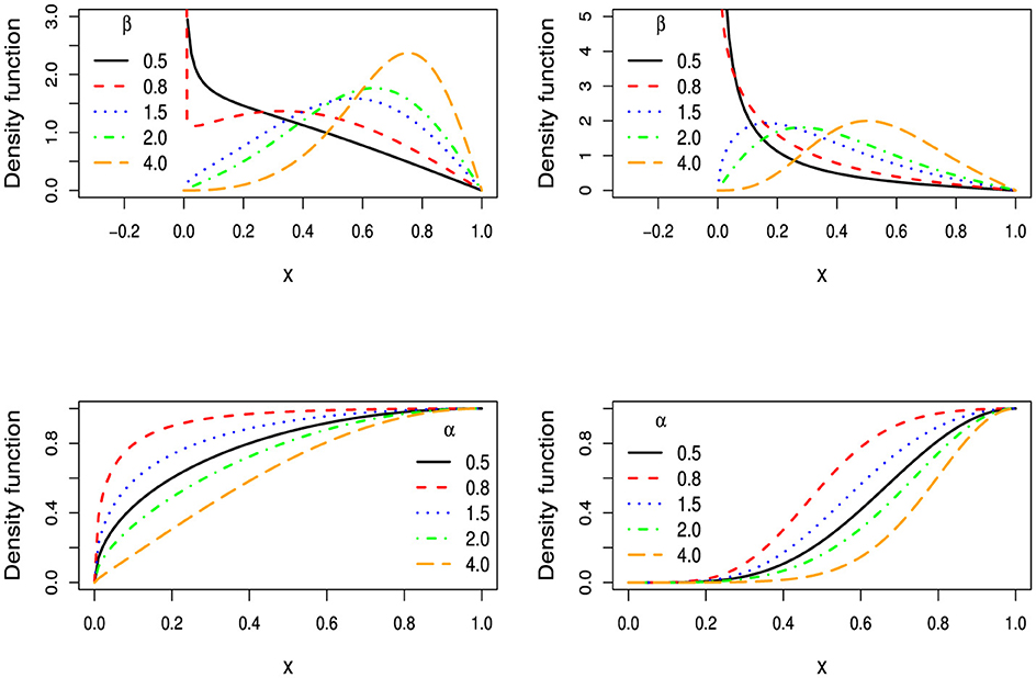
Figure 1. Some LTL PDF curves with b = 1 and different values for α and β.

Using Equation 8, LTL pseudo-random numbers can be generated straightforwardly by applying the inversion method. To facilitate this, we propose Algorithm 1.

Algorithm 1

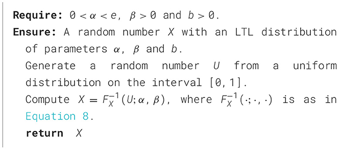
Algorithm 1. Lambert-Topp-Leone random number generation.

Figure 2 presents the histogram and cumulative distribution function for six sets of LTL pseudo-random numbers (three of size 50 and three of size 100,000), considering different values for the parameters α, β, and b. R codes [27] for the computation of Equations 7–9 are provided in Appendix 1.1. We use the function lamW::lambertW0() in the R programming language to compute the principal branch of the Lambert function W [28].

Figure 2

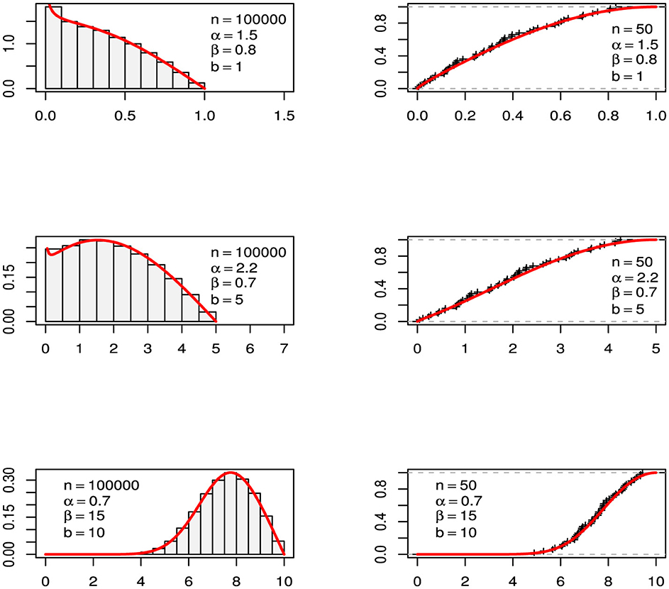
Figure 2. Histograms and cumulative distributions for six sets of LTL pseudo-random numbers generated with different values of α, β, and b, using sample sizes of n = 50 and n = 100, 000. In each panel, the red line represents the LTL PDF or the LTL CDF, as appropriate.

2.2 Moments and description of skewness and kurtosis

In this section, we derive the raw moments of the LTL distribution and use this result to describe the skewness and kurtosis behavior of the distribution.

Proposition 2. Let X ~ LTL(α, β, b). Then, for r = 1, 2, …, the rth moment of X is given by

$\begin{array}{ll}𝔼(X^r)=b^r{a}_r(\alpha ,\beta ),& (10)\end{array}$

where

$\begin{array}{l}{a}_r(\alpha ,\beta )={\displaystyle {\int }_0^1}{(1-\sqrt{1-u^{1/\beta }})}^r{\alpha }^u\left[1-log(\alpha )(1-u)\right]du.\end{array}$

Proof. From Equation 9, and by definition of expectation, we have that

$\begin{array}{r}𝔼(X^r)={\displaystyle {\int }_0^b}{x}^r\frac{2\beta }{b}y{(1-y^2)}^{\beta -1}{\alpha }^{{(1-y^2)}^{\beta }}\\ \left\{1-log(\alpha )\left[1-{(1-y^2)}^{\beta }\right]\right\}dx.\end{array}$

Thus, the result follows by considering the change of variable u = (1 − ^y2)β.

We employ the integrate() function of the R programming language to compute the function a_r(α, β) defined in Equation 10. Accordingly, the int() function is introduced to streamline the computation of a_r(α, β). For further details, refer to Appendix 1.1.

Corollary 1. Let X ~ LTL(α, β). Then, the mean (E(X)), variance (Var(X)), and skewness (S) and kurtosis (K) coefficients of X are given by

$𝔼(X)=b{a}_1,Var(X)=b^2(a_2-a_1^2),$

$S=\frac{a_3-3a_1{a}_2+a_1^3}{{(a_2-a_1^2)}^{3/2}}\text{and\hspace{1em}}K=\frac{a_4-4a_1{a}_3+6a_1^2{a}_2-3a_1^4}{{(a_2-a_1^2)}^2},$

where a_j = a_j(α, β), with j = 1, 2, 3, 4, is as in Proposition 2.

Figure 3 presents plots of the skewness and kurtosis coefficients of the LTL distribution. As shown in the figure, the highest values of skewness and kurtosis are obtained for small values of α and β.

Figure 3

Figure 3. Plots of the skewness and kurtosis coefficients of the LTL distribution.

2.3 Hazard rate function

As a direct consequence of Proposition 1, the following corollary proposes the hazard rate function (HRF) of the LTL distribution.

Corollary 2. Let X ~ LTL(α, β, b). The HRF of X is given by

$\begin{array}{l}{h}_X(x)={\displaystyle \underset{△x\to 0}{lim}}\frac{\mathbb{P}(x\le X<x+△x|X\ge x)}{△x}\\ =\frac{2\beta y{(1-y^2)}^{\beta -1}\left\{1-log(\alpha )\left[1-{(1-y^2)}^{\beta }\right]\right\}}{b\left[1-{(1-y^2)}^{\beta }\right]},\end{array}$

where y = 1 − x/b, 0 < x < b, b > 0, 0 < α < e and β > 0.

Remark 1. From Corollary 2, it can be seen that:

1. If α = 1, then

$\begin{array}{l}{h}_X(x)=\frac{2\beta }{b}\frac{y{(1-y^2)}^{\beta -1}}{1-{(1-y^2)}^{\beta }},y=1-\frac{x}{b},0<x<b,b,\beta >0,\end{array}$

that is the LT hrf.

2. If h_TL(x) represents the TL hrf, then

$\begin{array}{l}{\displaystyle \underset{x\to 0^{+}}{lim}}\frac{h_X(x)}{h_{\text{TL}}(x)}=1-log(\alpha )\text{and\hspace{1em}}{\displaystyle \underset{x\to 1^{-}}{lim}}\frac{h_X(x)}{h_{\text{TL}}(x)}=1.\end{array}$

Thus, the LTL hrf can be understood as a modification in the early times of the TL hrf.

Figure 4 presents several LTL hazard rate function (hrf) curves with b = 5 and different choices of α and β. As shown in the figure, the LTL hrf can exhibit both the bathtub shape (typical of the TL distribution) and an increasing shape.

Figure 4

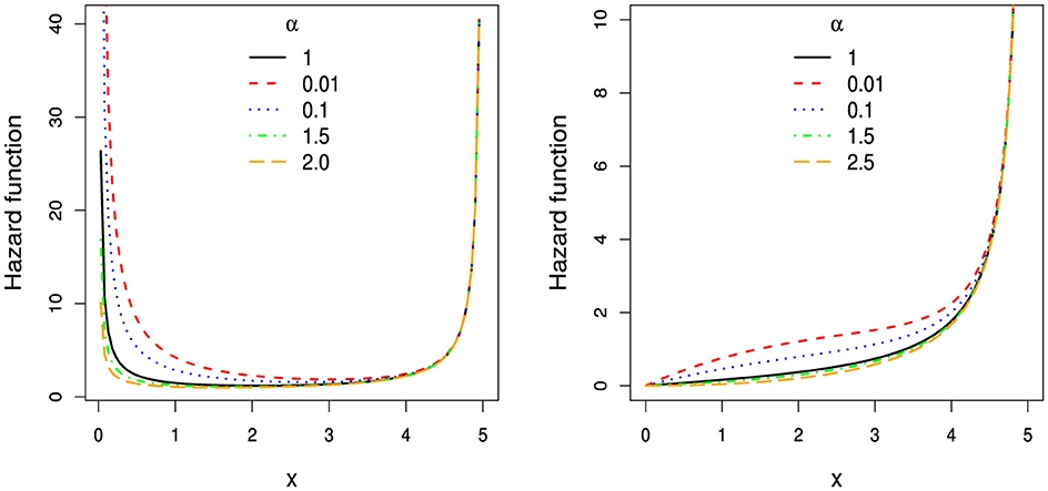
Figure 4. Plots of the hrf for the LTL distribution with- (b = 5, β = 0.5) in the left panel and (b = 5, β = 2.5) in the right panel.

The bathtub shape of a HRF characterizes a specific pattern of failure or event rates over time, commonly observed in reliability and survival analysis. This pattern consists of three distinct phases: (i) an initial phase with a decreasing hazard rate, dominated by early failures due to initial defects or weak components; (ii) a middle phase with an approximately constant hazard rate, representing the normal operational life of the system or product; and (iii) a final phase with an increasing hazard rate, attributed to wear-out, aging, or system deterioration.

Among the distributions in the literature that exhibit this shape, notable examples include the exponentiated Weibull [29], generalized gamma [30], beta [20], and Kumaraswamy [21] distributions. In Section 4, these distributions are utilized to assess the comparative performance of the LTL distribution in modeling real-world data.

3 Parameter estimation

In this section, we discuss the maximum likelihood (ML) estimation of the LTL distribution and evaluate its behavior using Monte Carlo simulation.

3.1 Maximum likelihood estimation

In this section, we discuss the maximum likelihood estimation for the LTL distribution, considering both cases where b are known and unknown. The case where b is known is particularly useful in scenarios where proportion data are being fitted, in which case b = 1 can be assumed. On the other hand, the case where b is unknown is useful in contexts that require fitting non-negative data, such as life data.

3.1.1 The case where b is known

Let X₁, X₂, …, X_n be a random sample of X ~ LTL(α, β, b), where b is known. Then, the log-likelihood function associated with θ = (α, β) is written as

$\begin{array}{l}\ell (\theta ;\text{x})=nlog(2)+nlog(\beta )-nlog(b)\\ +{\displaystyle \sum _{i=1}^n}log(y_i)+(\beta -1){\displaystyle \sum _{i=1}^n}log(1-y_i^2)\\ +log(\alpha ){\displaystyle \sum _{i=1}^n}{(1-y_i^2)}^{\beta }\\ +{\displaystyle \sum _{i=1}^n}log\{1-log(\alpha )[1-{(1-y^2)}^{\beta }]\},& (11)\end{array}$

where $\text{x}={(x_1,\dots ,x_n)}^{\text{T}}$ is the vector of observed values and y_i = 1 − x_i/b, for i = 1, …, n.

The ML estimator $\widehat{\theta }=(\widehat{\alpha },\widehat{\beta })$ of θ = (α, β) can be obtained by solving the system of equations given by the following score equations:

$\begin{array}{l}0=\frac{\partial \ell (\theta ;\text{x})}{\partial \alpha }={\displaystyle \sum _{i=1}^n}{(1-y_i^2)}^{\beta }-{\displaystyle \sum _{i=1}^n}\frac{1-{(1-y_i^2)}^{\beta }}{1-log(\alpha )[1-{(1-y_i^2)}^{\beta }]},\\ 0=\frac{\partial \ell (\theta ;\text{x})}{\partial \beta }=\frac{n}{\beta }+{\displaystyle \sum _{i=1}^n}log(1-y_i^2)\\ +log(\alpha ){\displaystyle \sum _{i=1}^n}log(1-y_i^2){(1-y_i^2)}^{\beta }\\ +log(\alpha ){\displaystyle \sum _{i=1}^n}\frac{log(1-y_i^2){(1-y_i^2)}^{\beta }}{1-log(\alpha )[1-{(1-y_i^2)}^{\beta }]}.\end{array}$

Since the root of this system do not have a closed form, the ML estimates for θ = (α, β) have to be obtained using numerical methods.

The standard errors of $\widehat{\theta }=(\widehat{\alpha },\widehat{\beta })$ can be obtained as the square roots of the elements of the diagonal of the matrix

${\text{K}}^{-1}(\widehat{\theta })={\left\{-\left(\begin{array}{l}\frac{{\partial }^2\ell (\theta ;\text{x})}{\partial {\alpha }^2}\frac{{\partial }^2\ell (\theta ;\text{x})}{\partial \alpha \partial \beta }\\ \frac{{\partial }^2\ell (\theta ;\text{x})}{\partial {\beta }^2}\end{array}\right){|}_{\theta =\widehat{\theta }}\right\}}^{-1},$

where

$\begin{array}{l}\frac{{\partial }^2\ell (\theta ;\text{x})}{\partial {\alpha }^2}=-\frac{1}{{\alpha }^2}{\displaystyle \sum _{i=1}^n}{(1-y_i^2)}^{\beta }\\ +\frac{1}{{\alpha }^2}{\displaystyle \sum _{i=1}^n}\frac{1-{(1-y_i^2)}^{\beta }}{1-log(\alpha )\left[1-{(1-y_i^2)}^{\beta }\right]}\\ -\frac{1}{{\alpha }^2}{\displaystyle \sum _{i=1}^n}\frac{{\left[1-{(1-y_i^2)}^{\beta }\right]}^2}{{\left\{1-log(\alpha )\left[1-{(1-y_i^2)}^{\beta }\right]\right\}}^2},\\ \frac{{\partial }^2\ell (\theta ;\text{x})}{\partial \alpha \partial \beta }=\frac{1}{\alpha }{\displaystyle \sum _{i=1}^n}{(1-y_i^2)}^{\beta }log(1-y_i^2)\\ +\frac{1}{\alpha }{\displaystyle \sum _{i=1}^n}\frac{{(1-y_i^2)}^{\beta }log(1-y_i^2)}{1-log(\alpha )\left[1-{(1-y_i^2)}^{\beta }\right]}\\ \\ +\frac{log(\alpha )}{\alpha }{\displaystyle \sum _{i=1}^n}\frac{{(1-y_i^2)}^{\beta }\left[1-{(1-y_i^2)}^{\beta }\right]log(1-y_i^2)}{{\left\{1-log(\alpha )\left[1-{(1-y_i^2)}^{\beta }\right]\right\}}^2},\\ \frac{{\partial }^2\ell (\theta ;\text{x})}{\partial {\beta }^2}=-\frac{n}{\beta }+log(\alpha ){\displaystyle \sum _{i=1}^n}{(1-y_i^2)}^{\beta }{log}^2(1-y_i^2)\\ +log(\alpha ){\displaystyle \sum _{i=1}^n}\frac{{(1-y_i^2)}^{\beta }{log}^2(1-y_i^2)}{1-log(\alpha )\left[1-{(1-y_i^2)}^{\beta }\right]}\\ -{log}^2(\alpha ){\displaystyle \sum _{i=1}^n}\frac{{(1-y_i^2)}^{2\beta }{log}^2(1-y_i^2)}{{\left\{1-log(\alpha )\left[1-{(1-y_i^2)}^{\beta }\right]\right\}}^2}.\end{array}$

Alternatively, to obtain ML estimates of θ = (α, β), it is possible to solve the problem of maximizing Equation 11 with the help of some numerical optimization routine such as the function stats:optim() of the R programming language [27]. In this case, minimizing the negative log-likelihood, this function returns the ML estimates and the numerical Hessian matrix. R codes for the computation of Equation 11 and for its maximization are provided in Appendix 1.1.

3.1.2 The case where b is unknown

Let X₁, X₂, …, X_n be a random sample of X ~ LTL(α, β, b), where α, β, and b are unknown. In this case, the ML estimator for b is $\widehat{b}=T(\text{x})=max(\text{x})$, where $\text{x}={(x_1,x_2,\dots ,x_n)}^T$ is the vector of observed values.

It should be noted that the PDF of T(X) = max(X) is $g_{T(\text{X})}(x)=ng(x){\left[G(x)\right]}^{n-1}$, where G(x) = G(x; α, β, b) and g(x) = g(x; α, β, b) are as in Equations 7, 9, respectively. So, the PDF of T(X) can be written as

$\begin{array}{l}{g}_{T(\text{X})}(x)=\frac{2n\beta }{b}y{(1-y^2)}^{\beta -1}{\alpha }^{{(1-y^2)}^{\beta }}\\ \left\{1-log(\alpha )\left[1-{(1-y^2)}^{\beta }\right]\right\}\\ \times {\left\{1-\left[1-{(1-y^2)}^{\beta }\right]{\alpha }^{{(1-y^2)}^{\beta }}\right\}}^{n-1},\end{array}$

where 0 < x < b, 0 < α < e, β > 0, b > 0, and n ∈ ℕ. Thus, the rth raw moment of T(X) is given by

$\begin{array}{l}{\mu }_r=𝔼\left[T{(\text{X})}^r\right]={\displaystyle {\int }_0^b}{x}^r{g}_{T(\text{X})}(x)dx,r=1,2,3,\dots \end{array}$

Then, the variance of T(X) is $V\left[T(\text{X})\right]={\mu }_2-{\mu }_1^2$, so the standard error of $\widehat{b}=T(\text{x})=max(\text{x})$ is

$\begin{array}{ll}\text{se}(\widehat{b})=\sqrt{V\left[T(\text{x})\right]}=\sqrt{{\mu }_2-{\mu }_1^2}.& (12)\end{array}$

We compute Equation 12 in the R programming language, see Appendix 1.1 for code details.

Once the ML estimate of b has been calculated, the ML estimates of α and β can be calculated considering b as known, as illustrated in Section 3.1.1.

3.2 Simulation studies

This section presents the results of two simulation studies designed to evaluate the performance of the ML estimators for the LTL distribution parameters and assess the overall fitting performance in the presence of outliers.

3.2.1 Performance evaluation of parameter estimators

In this section, a simulation study is carried out to evaluate the performance of ML estimators for the parameters of the LTL distribution. We generated 1,000 random samples from the LTL distribution for each of the sample sizes n = 100, 200, 300, 500, 1,000, and 2,000. The pseudo-random numbers were generated using the inversion method discussed in Section 2.1, and we considered the simulation scenarios presented in Table 1.

Table 1

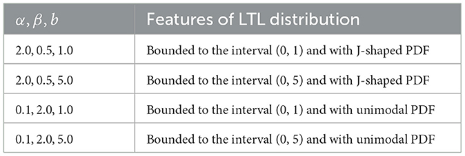
Table 1. Simulation scenarios.

For each generated sample, we compute the ML estimator for the parameters of the LTL distribution, considering the results of Section 3.1.2. Table 2 reports the average estimates and standard deviations obtained in each simulation scenario. From the table, it can be seen that the average estimates approach the true values of the parameters and the standard deviations decrease to 0 as the sample size increases, which demonstrates the consistency of the estimators.

Table 2

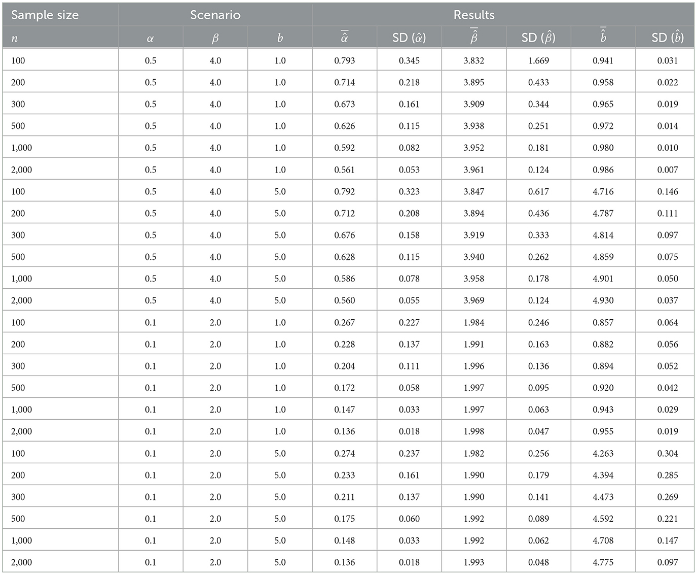
Table 2. Averages and standard deviations of the ML estimates obtained in each simulation scenario under the different sample sizes.

3.2.2 Performance evaluation of the LTL distribution under outlier observations

The objective of this section is to evaluate the performance of the LTL distribution in the presence of outlier observations. Specifically, we analyze the distribution's robustness and fitting accuracy through simulations under different scenarios and sample sizes.

We consider two distinct simulation scenarios for generating pseudo-random numbers from the LTL distribution. In Scenario 1, the parameters are (α = 2, β = 3, b = 5), where the PDF is unimodal and exhibits a Fisher kurtosis value of 2.706 (PDF with light tails). In Scenario 2, the parameters are (α = 0.1, β = 0.5, b = 5), where the PDF is decreasing and exhibits a kurtosis value of 14.524 (PDF with heavy tails). In both scenarios, 1,000 pseudo-random samples were generated from the LTL distribution for sample sizes n = 100, 200, 300, 400, and 500.

For each generated sample, outliers were identified using the interquartile range (IQR) criterion. Specifically, an observation was considered an outlier if it fell outside the range (i, s), where i = q₁−1.5(q₃−q₁), s = q₃+1.5(q₃−q₁), and q₁ and q₂ represent the first and third sample quartiles, respectively.

To evaluate the performance of the LTL distribution, the Kolmogorov–Smirnov (KS) goodness-of-fit test was applied to each sample. The test assesses the agreement between the empirical distribution and the theoretical LTL distribution. A sample was deemed appropriately fitted if the KS test yielded a p-value greater than 0.05. The ML estimates of the LTL distribution parameters were obtained based on the results from Section 3.1.2.

For each set of 1,000 simulated samples, the following metrics were calculated:

1. Outlier presence: the percentage of samples that exhibited at least one outlier based on the IQR criterion.

2. Success percentage: the percentage of samples appropriately fitted with the LTL distribution (p-value > 0.05 in the Kolmogorov–Smirnov (KS) test [31]).

These metrics provide insights into the LTL distribution's capability to handle outlier observations and its overall fitting performance across different simulation scenarios and sample sizes.

Table 3 presents the results for each set of 1,000 simulated samples. It can be observed that in Scenario 1, the predominance of outliers is lower compared to Scenario 2, primarily due to differences in the weight of the PDF tails in each scenario. Notably, the success rates exceed 92%, indicating that the presence of outliers does not adversely affect the performance of the LTL distribution. Interestingly, the success rate increases as the proportion of samples containing outliers grows.

Table 3

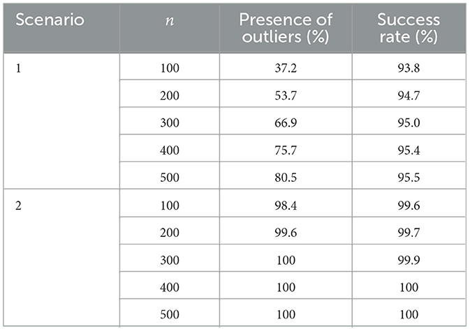
Table 3. Percentages of outlier presence and success rates obtained from 1,000 simulated samples for each scenario and sample size considered.

4 Data analysis

In this section, we illustrate the utility of the LTL distribution through two application examples in different real-world settings. In the first example, we employ the LTL distribution to fit a proportion data set, comparing its performance to the beta (B) [32] and Kumaraswamy (K) [21] distributions, which are two of the earliest alternatives used to fit this type of data. In the second example, we employ the LTL distribution to fit a fatigue life data set, where we compare its performance to six lifetime distributions: the Weibull (W) [23], generalized exponential (GE) [25], Birnbaum-Saunders (BS) [24], generalized Rayleigh (GR) [26], exponentiated Weibull (EW) [29], generalized gamma (GG) [30], Rayleigh (R) [20], and exponential (E) [20] distributions. The PDFs of these distributions are presented in Appendix 1.2.

We employ the Kolmogorov–Smirnov (KS) and Cramer-von Mises (CvM) goodness-of-fit tests to assess the quality of the fits. For this, we use the stats::ks.test() and goftest::cvm.test() functions of the R programming language. In addition, we employ the excess mass test proposed by Ameijeiras-Alonso et al. [33] to show the unimodality of the data considered in each application example. More specifically, we test the hypothesis H₀ (the data has exactly one mode) versus the alternative hypothesis H₁ (the data has at least two modes). For this, we use the function multimode::modetest [34] in the R programming language.

4.1 Family spending on food

Family spending on food is an important component of the family budget, and its amount can vary significantly by factors such as geographic location, family size, and dietary preferences, to name a few. In industry, knowledge about household food spending helps companies make informed decisions about products, pricing, marketing, and distribution strategies. This allows them to better meet the needs of consumers and remain competitive in the market.

In this section, we analyze a dataset of 1,519 observations on the proportion of the British household budget allocated to food. These data are available as BudgetUK (wfood) in the Ecdat package of the R programming language [35]. A descriptive analysis reveals that the minimum and maximum values are 0.0571 and 0.7890, with Fisher skewness and kurtosis values of 0.147 and 2.899, respectively. In addition, the excess mass test yields a p-value of 0.376, indicating that, at conventional significance levels, the hypothesis that the frequency distribution of these data is unimodal is not rejected. Consequently, the LTL distribution with b = 1 appears to be a viable alternative for modeling these data.

Table 4 reports the ML estimates for the parameters of the LTL, B, K, and TL distributions fitted to the data on the proportion of the shared household budget spent on food. The results obtained in the KS and CvM goodness-of-fit tests are also presented in Table 4 for each distribution. Note that the LTL distribution exhibits a larger p-value, indicating that this distribution performs better in fitting the data.

Table 4

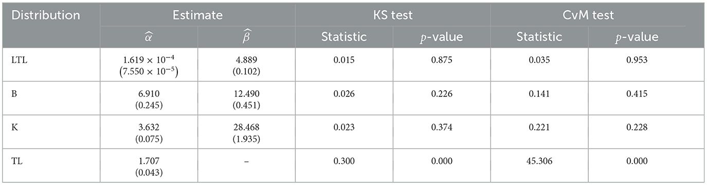
Table 4. Maximum likelihood (ML) estimates, observed statistics, and p-values obtained from goodness-of-fit tests for distributions fitted to the proportion of household expenditure allocated to food.

By computing probabilities using the LTL distribution, we observe that, in the analyzed population, a family is likely to allocate at most 25%, 50%, and 75% of their shared family budget to food with probabilities of 0.1572, 0.9110, and 0.9995, respectively.

Figure 5 presents the histogram of the proportion of household expenditure allocated to food, along with the PDFs of the fitted distributions. The figure illustrates that the LTL PDF aligns more closely with the empirical frequency values, particularly around the mode.

Figure 5

Figure 5. Histogram of the proportion of household shared expenditure on food along with the fitted PDFs.

4.2 Fatigue life data

Analyzing fatigue life data is crucial in engineering, materials, and data science applied to predicting the failure time of components and structures subjected to load cycles. These data help to understand how a material's performance degrades over time due to repetitive loading, which is essential for the safety and efficiency of structures such as bridges, aircraft, automobiles, and industrial machinery.

We consider 101 observations on the fatigue life of 6061-T6 aluminum coupons cut parallel to the direction of rolling and oscillated at 18 cycles per second. These data were originally analyzed in Birnbaum and Saunders [24] and are currently available under the name “fatigue” in the bibs package of the R programming language.

A descriptive analysis of the data indicates that the minimum and maximum observed values are 70 and 212, respectively, with Fisher skewness and kurtosis values of 0.3 and 4.1. In addition, the excess mass test yields a p-value of 0.686, suggesting that the hypothesis of unimodality for the frequency distribution of the fatigue life data is not rejected at conventional significance levels. Consequently, the LTL distribution with an unspecified parameter b appears to be a viable alternative for modeling these data.

Figure 6 presents the quantile-quantile plot (Q–Q plot) of the fatigue life data, revealing the presence of outliers, two of which are located at the upper end of the data range. It is important to highlight that outliers can adversely affect the modeling process using the LTL distribution as the parameter b is estimated as the maximum value of the sample. This estimation may unnecessarily expand the support of the distribution and potentially impact its fit to the remaining data. This raises a critical question: can the LTL distribution still provide an appropriate fit for the fatigue life data despite the presence of these outlier observations?

Figure 6

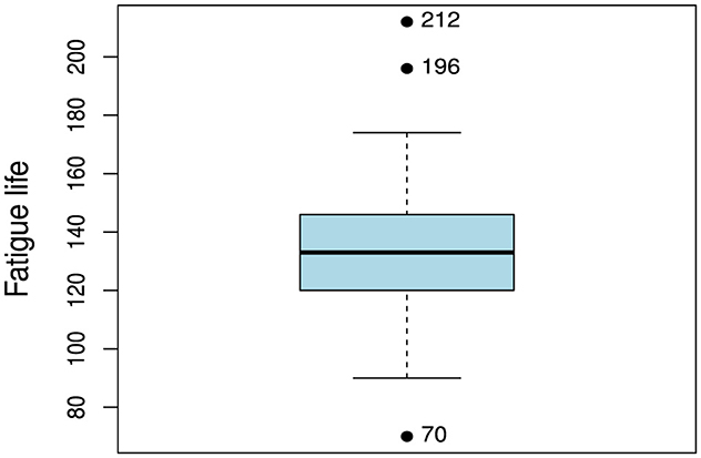
Figure 6. Q–Q plot of the fatigue life data.

Table 5 reports the ML estimates for the parameters of the LTL, W, GE, BS, GR, EW, GG, R, and E distributions fitted to the fatigue life data. The results obtained in the KS and CvM goodness-of-fit tests are also presented in Table 5 for each distribution. Note that the LTL distribution exhibits a larger p-value, indicating that this distribution performs better in fitting the data.

Table 5

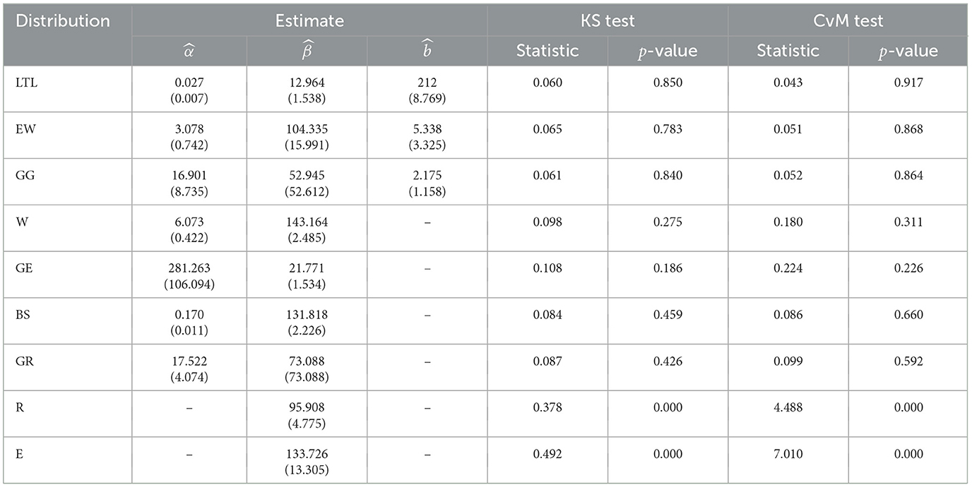
Table 5. Maximum likelihood (ML) estimates, observed statistics, and p-values obtained from goodness-of-fit tests for distributions fitted to the fatigue life data.

Figure 7 (left panel) presents the histogram of the fatigue life data, along with the PDFs of the fitted distributions. The figure illustrates that the LTL PDF aligns more closely with the empirical frequency values, particularly around the mode. In the right panel of Figure 7, the HRFs of the distributions fitted to the fatigue life data are presented, where a similar behavior can be observed for the LTL, W, EW, and GG distributions, but differing significantly for a fatigue life value > 50.

Figure 7

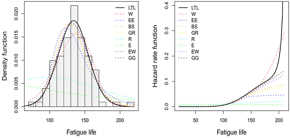
Figure 7. (Left) Histogram of fatigue life data along with fitted PDFs. (Right) HRFs for the distributions fitted to the fatigue life data.

Regarding the earlier question about the presence of outlier observations, the results demonstrate that the LTL distribution performs robustly in modeling the fatigue life data, even under the influence of the outliers. Notably, its performance surpasses that of several established lifetime distributions from the literature, highlighting its flexibility in this challenging scenario.

5 Discussion and further research

As demonstrated throughout this article, the new LTL distribution exhibits several strengths, which are summarized as follows.

The LTL distribution inherits the shapes of the PDF and the HRF from the baseline TL distribution. However, the additional parameter α, introduced by the Lambert-F generator, enhances its flexibility, allowing the LTL distribution to exhibit wider ranges of skewness and kurtosis. This makes it a valuable alternative in scenarios where empirical skewness and/or kurtosis levels cannot be adequately captured by the TL distribution.

The new LTL distribution is defined by three parameters: two shape parameters (α and β) and one support-bounding parameter (b). When b = 1, the LTL distribution becomes a suitable alternative for modeling proportion data. In this context, it serves as a natural competitor to the widely used beta (B) and Kumaraswamy (K) distributions. This study demonstrates this by fitting the LTL distribution to a real-world dataset, showing that it can outperform the B and K distributions in modeling the data.

When b is unknown, the LTL distribution is suitable for modeling positive data, such as lifetime data. In this context, it serves as a competitor to well-known lifetime distributions, including the exponentiated Weibull (EW) and generalized gamma (GG) distributions. This study demonstrates this by fitting the LTL distribution to a fatigue failure dataset, showing that it can outperform the EW and GG distributions in modeling the data.

A disadvantage of the new LTL distribution is that, unlike the baseline TL distribution, properties such as the PDF, HRF, and moments have a more complex analytical structure. While properties such as the PDF and HRF are manageable, its moments require numerical integration for their computation. To address this difficulty, we have provided R code for computing these properties, which is accessible to readers.

Regarding the estimation of the support-bounding parameter of the LTL distribution, estimating it as the maximum value of the sample can pose challenges. The presence of outliers may artificially inflate the support, introducing biases in the model fit, hindering an accurate representation of the data structure, and compromising the stability and precision of the estimates, particularly in samples with high dispersion. In this study, Monte Carlo simulations have shown that the LTL distribution performs well in the presence of outliers when the samples are generated from an LTL distribution. This suggests that real-world scenarios may exist where the LTL distribution effectively models data with outliers, adequately capturing empirical properties such as unimodality and skewness. This is precisely what is illustrated in Section 4.2.

As ideas for future research, we propose the following:

First, it would be worthwhile to explore alternative estimation methods for the parameters of the LTL distribution. In particular, the results from Section 2.2 could be utilized to derive moment estimators and compare their performance with maximum likelihood estimators.

Second, starting from the LTL quantile function, a quantile regression framework can be formulated. By considering θ = G⁻¹(p; α, β, b), where G⁻¹(·;·, ·, ·) is defined as in Equation 8, we can express

$\alpha ={\left(\frac{p-1}{{\left[1-{\left(1-\frac{\theta }{b}\right)}^2\right]}^{\beta }}\right)}^{\frac{1}{{\left[1-{\left(1-\frac{\theta }{b}\right)}^2\right]}^{\beta }+1}}.$

The PDF in Equation 9 can then be re-parameterized in terms of the p-th quantile (with p fixed). This re-parameterized PDF provides the foundation for a regression model to quantify the relationship between a set of explanatory variables and the p-th quantile of a positive response variable.

6 Final comment

This study introduces the Lambert-Topp-Leone (LTL) distribution as a flexible model for bounded and positive skewed data, particularly suitable for proportion and lifetime data. The LTL distribution extends the Topp-Leone distribution by incorporating an additional shape parameter, thereby enhancing its flexibility to accommodate a wider range of skewness and kurtosis. Our findings suggest that the LTL distribution provides an improved fit over traditional models, as demonstrated through real-world applications involving household spending proportions and fatigue life data. The simulation studies further confirm the consistency and robustness of maximum likelihood estimators for the LTL parameters, adding to its practical utility. A second simulation study has shown that the LTL distribution performs robustly in the presence of outliers.

Given its adaptability, the LTL distribution holds promise for diverse applications beyond the examples explored here, potentially benefiting fields that require accurate modeling of constrained or positively skewed datasets. Future research could focus on exploring Bayesian estimation methods, assessing the performance of the distribution with diverse data types, and developing quantile regression frameworks based on the new distribution to expand its applicability.

Data availability statement

Publicly available datasets were analyzed in this study. The data are available in the R programming language, and details on their location are provided in the article.

Author contributions

JA: Conceptualization, Data curation, Formal analysis, Investigation, Methodology, Resources, Software, Supervision, Validation, Visualization, Writing – original draft, Writing – review & editing. YI: Conceptualization, Data curation, Formal analysis, Investigation, Methodology, Resources, Software, Supervision, Validation, Visualization, Writing – original draft, Writing – review & editing.

Funding

The author(s) declare that no financial support was received for the research, authorship, and/or publication of this article.

Conflict of interest

The authors declare that the research was conducted in the absence of any commercial or financial relationships that could be construed as a potential conflict of interest.

Generative AI statement

The author(s) declare that no Gen AI was used in the creation of this manuscript.

Publisher's note

All claims expressed in this article are solely those of the authors and do not necessarily represent those of their affiliated organizations, or those of the publisher, the editors and the reviewers. Any product that may be evaluated in this article, or claim that may be made by its manufacturer, is not guaranteed or endorsed by the publisher.

Supplementary material

The Supplementary Material for this article can be found online at: https://www.frontiersin.org/articles/10.3389/fams.2025.1527833/full#supplementary-material

References

1. Topp CW, Leone FC. A family of J-shaped frequency functions. J Am Stat Assoc. (1955) 50:209–19. doi: 10.1080/01621459.1955.10501259

Crossref Full Text | Google Scholar

2. Nadarajah S, Kotz S. Moments of some J-shaped distributions. J Appl Stat. (2003) 30:311–7. doi: 10.1080/0266476022000030084

Crossref Full Text | Google Scholar

3. Ghitany M, Kotz S, Xie M. On some reliability measures and their stochastic orderings for the Topp-Leone distribution. J Appl Stat. (2005) 32:715–22. doi: 10.1080/02664760500079613

Crossref Full Text | Google Scholar

4. Zhou M, Yang D, Wang Y, Nadarajah S. Some J-shaped distributions: sums, products and ratios. In: RAMS'06. Annual Reliability and Maintainability Symposium, 2006. IWashington, DC: EEE (2006), p. 175–81. doi: 10.1109/RAMS.2006.1677371

Crossref Full Text | Google Scholar

5. Kotz S, Seier E. Kurtosis of the Topp-Leone distributions. Interstat. (2007) 1:1–15.

Google Scholar

6. Nadarajah S. Bathtub-shaped failure rate functions. Qual Quant. (2009) 43:855–63. doi: 10.1007/s11135-007-9152-9

Crossref Full Text | Google Scholar

7. Genç AĨ. Moments of order statistics of Topp-Leone distribution. Stat Pap. (2012) 53:117–31. doi: 10.1007/s00362-010-0320-y

Crossref Full Text | Google Scholar

8. Marshall AW, Olkin I. A new method for adding a parameter to a family of distributions with application to the exponential and Weibull families. Biometrika. (1997) 84:641–52. doi: 10.1093/biomet/84.3.641

Crossref Full Text | Google Scholar

9. Eugene N, Lee C, Famoye F. Beta-normal distribution and its applications. Commun Stat-Theory Methods. (2002) 31:497–512. doi: 10.1081/STA-120003130

Crossref Full Text | Google Scholar

10. Zografos K, Balakrishnan N. On families of beta-and generalized gamma-generated distributions and associated inference. Stat Methodol. (2009) 6:344–62. doi: 10.1016/j.stamet.2008.12.003

Crossref Full Text | Google Scholar

11. Shaw WT, Buckley IR. The alchemy of probability distributions: beyond Gram-Charlier expansions, and a skew-kurtotic-normal distribution from a rank transmutation map. arXiv. (2009). [Preprint]. arXiv:0901:0434. doi: 10.48550/arXiv.0901:0434

Crossref Full Text | Google Scholar

12. Cordeiro GM, de Castro M. A new family of generalized distributions. J Stat Comput Simul. (2011) 81:883–98. doi: 10.1080/00949650903530745

Crossref Full Text | Google Scholar

13. Alzaatreh A, Lee C, Famoye F. A new method for generating families of continuous distributions. Metron. (2013) 71:63–79. doi: 10.1007/s40300-013-0007-y

Crossref Full Text | Google Scholar

14. Mahdavi A, Kundu D. A new method for generating distributions with an application to exponential distribution. Commun Stat Theory Methods. (2017) 46:6543–57. doi: 10.1080/03610926.2015.1130839

Crossref Full Text | Google Scholar

15. Atchadé MN, Agbahide AA, Otodji T, Bogninou MJ, Moussa Djibril A. A new shifted Lomax-X family of distributions: properties and applications to actuarial and financial data. Comput J Math Stat Sci. (2025) 4:41–71. doi: 10.21608/cjmss.2024.307114.1066

PubMed Abstract | Crossref Full Text | Google Scholar

16. Iriarte YA, de Castro M, Gómez HW. The Lambert-F distributions class: an alternative family for positive data analysis. Mathematics. (2020) 8:1398. doi: 10.3390/math8091398

Crossref Full Text | Google Scholar

17. Iriarte YA, de Castro M, Gómez HW. An alternative one-parameter distribution for bounded data modeling generated from the Lambert transformation. Symmetry. (2021) 13:1190. doi: 10.3390/sym13071190

Crossref Full Text | Google Scholar

18. Iriarte YA, de Castro M, Gómez HW. A unimodal/bimodal skew/symmetric distribution generated from Lambert's transformation. Symmetry. (2021) 13:269. doi: 10.3390/sym13020269

Crossref Full Text | Google Scholar

19. Varela H, Rojas MA, Reyes J, Iriarte YA. An alternative Lambert-type distribution for bounded data. Mathematics. (2023) 11:667. doi: 10.3390/math11030667

Crossref Full Text | Google Scholar

20. Johnson NL, Kotz S, Balakrishnan N. Continuous Univariate Distributions, Vol. 1, 2nd Edn. New York, NY: Wiley (1994).

PubMed Abstract | Google Scholar

21. Kumaraswamy P. A generalized probability density function for double-bounded random processes. J. Hydrol. (1980) 46:79–88. doi: 10.1016/0022-1694(80)90036-0

Crossref Full Text | Google Scholar

22. Irshad M, Aswathy S, Maya R, Al-Omari AI, Alomani G. A flexible model for bounded data with bathtub shaped hazard rate function and applications. AIMS Math. (2024) 9:24810–31. doi: 10.3934/math.20241208

Crossref Full Text | Google Scholar

23. Weihull W. A statistical distribution function of wide applicability. J Appl Mech. (1951) 18:290–3. doi: 10.1115/1.4010337

Crossref Full Text | Google Scholar

24. Birnbaum ZW, Saunders SC. A new family of life distributions. J Appl Probab. (1969) 6:319–27. doi: 10.1017/S0021900200032848

Crossref Full Text | Google Scholar

25. Gupta RD, Kundu D. Exponentiated exponential family: an alternative to gamma and Weibull distributions. Biom J. (2001) 43:117–30. doi: 10.1002/1521-4036(200102)43:1&lt;117::AID-BIMJ117&gt;3.0.CO;2-R

Crossref Full Text | Google Scholar

26. Surles J, Padgett W. Inference for reliability and stress-strength for a scaled Burr Type X distribution. Lifetime Data Anal. (2001) 7:187–200. doi: 10.1023/A:1011352923990

PubMed Abstract | Crossref Full Text | Google Scholar

27. R Core Team. R: A Language and Environment for Statistical Computing. Vienna (2023). Available at: https://www.R-project.org/ (accessed February 8, 2025).

Google Scholar

28. Adler A. lamW: Lambert-W Function. R package version 2.2.3. (2015). Available at: https://CRAN.R-project.org/package=lamW (accessed February 8, 2025).

Google Scholar

29. Mudholkar GS, Hutson AD. The exponentiated Weibull family: some properties and a flood data application. Commun Stat-Theory Methods. (1996) 25:3059–83. doi: 10.1080/03610929608831886

Crossref Full Text | Google Scholar

30. Stacy EW. A generalization of the gamma distribution. Ann Math Stat. (1962) 33:1187–92. doi: 10.1214/aoms/1177704481

Crossref Full Text | Google Scholar

31. Faraway J, Marsaglia G, Marsaglia J, Baddeley A. goftest: Classical Goodness-of-Fit Tests for Univariate Distributions. R package version 1.2-3. (2021). Available at: https://CRAN.R-project.org/package=goftest (accessed February 8, 2025).

Google Scholar

32. Johnson NL, Kotz S, Balakrishnan N. Continuous Univariate Distributions, Volume 2, 2nd Edn. New York, NY: Wiley (1995).

Google Scholar

33. Ameijeiras-Alonso J, Crujeiras RM, Rodríguez-Casal A. Mode testing, critical bandwidth and excess mass. Test. (2019) 28:900–19. doi: 10.1007/s11749-018-0611-5

Crossref Full Text | Google Scholar

34. Ameijeiras-Alonso J, Crujeiras RM, Rodríguez-Casal A. multimode: an R package for mode assessment. J Stat Softw. (2021) 97:1–32. doi: 10.18637/jss.v097.i09

Crossref Full Text | Google Scholar

35. Croissant Y, Graves S. Ecdat: Data Sets for Econometrics. R package version 0.4-2. (2022). Available at: https://CRAN.R-project.org/package=Ecdat (accessed February 8, 2025).

Google Scholar