Computation and interpretation of mean absolute deviations by cumulative distribution functions

In recent years, there has been an increased interest in using the mean absolute deviation (MAD) around the mean and median (the L₁ norm) as an alternative to standard deviation σ (the L₂ norm). Till now, the MAD has been computed for some distributions. For other distributions, expressions for mean absolute deviations (MADs) are not available nor reported. Typically, MADs are derived using the probability density functions (PDFs). By contrast, we derive simple expressions in terms of the integrals of the cumulative distribution functions (CDFs). We show that MADs have simple geometric interpretations as areas under the appropriately folded CDF. As a result, MADs can be computed directly from CDFs by computing appropriate integrals or sums for both continuous and discrete distributions, respectively. For many distributions, these CDFs have a simpler form than PDFs. Moreover, the CDFs are often expressed in terms of special functions, and indefinite integrals and sums for these functions are well known. We compute MADs for many well-known continuous and discrete distributions. For some of these distributions, the expressions for MADs have not been reported. We hope this study will be useful for researchers and practitioners interested in MADs.

1 Introduction

Consider a real-valued random variable X on a sample space Ω ⊆ R with density f(x) and cumulative distribution function F(x) [1]. If X is a discrete random variable, then Ω is some countable sample space and f(x) is the probability mass function (discrete density function). Let μ denote the mean E(X) and M denote the median of X. For any real-value a, define the MAD of X from a as Bloomfield and Steiger [2]

$\begin{array}{ll}H(X,a)={\displaystyle {\int }_{\Omega }|x-a|dF(x)}& (1)\end{array}$

This is defined in Lebesque–Stieltjes integration [3] and applies to continuous and discrete distributions. It is well known [2, 4–6] that for any distribution with finite variance, we have H(X, M) ≤ H(X, μ) ≤ σ. On the other hand, MADs require only the existence of the first-order moment.

MADs have been used for a long time, as early as the eighteenth century by Boscovitch and Laplace [7, 8]. For a historical survey, see Gorard [9] and Pham-Gia and Hung [10]. There is currently a renewed interest in using the L₁ norm for robust statistical modeling and inference (e.g. [11–17], to name just a few). A MAD-based alternative to kurtosis based on H(X, M) was recently introduced in Pinsky and Klawansky [18].

Since the pioneering work of Fisher [19], standard deviation has been used as the primary metric for deviation. As noted in Gorard [9] and Pham-Gia and Hung [10], the convenience of differentiation and optimization, and the summation of variances for independent variables have contributed to the widespread use of the standard deviation in estimation and hypothesis testing.

On the other hand, using MAD offers a direct measure of deviation and is more resilient to outliers. In computing standard deviation, we square the differences between values and the central point such as mean or median. As a result, standard deviation emphasizes larger deviations. The computation of MAD offers a direct and easily interpretable measure of deviation.

As discussed in Gorard [9], difficulties associated with the absolute value operation are one of the main reasons for the lower use of the MAD. We address this by deriving the closed-form expressions for MADs directly from the cumulative distribution function of the underlying distribution. Moreover, the computation of MAD requires only the existence of the first-order moment, whereas the use of standard deviation requires the existence of the second moment as well. As an example, consider Pareto distribution with scale α [20] analyzed in Section 5. This distribution has a finite mean for α > 1 but the infinite variance for α < 2. As a result, we cannot use standard deviation to analyze cases 1 < α < 2 but can use MADs.

This study will primarily focus on computing the MAD about the mean. Such deviations have been derived for some distributions, primarily using density [21]. The most complete list (without derivations) is presented in Weisstein [22]. We significantly extend this list using a unified approach to computing these deviations as integrals and sums from cumulative distribution functions (CDFs) instead of probability density functions (PDFs). For many distributions, these CDFs have a simpler form than PDFs. Moreover, the CDFs are often expressed in terms of special functions, and indefinite integrals and sums for these functions are well known. When closed-form expressions for the median are available, we will compute MAD (about) median as well.

To our knowledge, the obtained results for some distributions, such as Pareto Type II, and logarithmic distributions, are presented for the first time. Our main contribution is a unified and simple computational approach to compute these deviations in closed form without absolute value operation from the cumulative distribution functions. This removes one of the main obstacles in using MADs [9]. We hope this article will be a useful reference for researchers and practitioners using MAD.

This article is organized as follows. In Section 2, we establish the expressions for H(X, μ) in terms of the integral of the CDF for the case of continuous distributions and in terms of sums of the CDFs for discrete distributions. In Section 3, we provide a simple geometric interpretation of our results in terms of appropriately folded CDF. In Section 4, we review definitions and some integrals for the special functions often appearing in CDFs for many distributions considered. In Section 5, we derive expressions for MAD for many continuous distributions. In Section 6, we derive expressions for many widely used discrete distributions.

2 Computing MADs by CDF

2.1 MAD formula for continuous distributions

We first start with continuous distributions. Let us define the left sample sub-space of Ω by Ω_L(a) = {x ∈ Ω | x ≤ a} and the right sample sub-space of Ω by Ω_R(a) = {x ∈ Ω | x > a}. Additionally, we will require the existence of the first-order moment,

$\begin{array}{ll}\mu ={\displaystyle {\int }_{x\in \Omega }}xdF(x)={\displaystyle {\int }_{x\in {\Omega }_L}}xdF(x)+{\displaystyle {\int }_{x\in {\Omega }_R}}xdF(x)<\infty & (2)\end{array}$

To put it formally, let us consider the functional [23]

$\begin{array}{ll}L(X,t)={\displaystyle {\int }_{-t}^a}\left|x\right|dF(x)+{\displaystyle {\int }_a^t}\left|x\right|dF(x)& (3)\end{array}$

where a ∈ (−t, t) is finite and both integrals exist for any t. Then the first moment is defined as

$\begin{array}{ll}\mu ={\displaystyle \underset{t\mapsto \infty }{lim}}L(X,t)& (4)\end{array}$

It is well known that the integral in Equation 3 could be infinite when the support of X is unbounded. We will insist that the above integrals in the right-hand side of the above Equation 2 are finite and therefore μ < ∞. This can be shown to be equivalent:

$\begin{array}{r}\underset{t\mapsto \infty }{\lim }tP(|X|\ge t)=\underset{t\mapsto \infty }{\lim }t(1-P(\left|X\right|\le t)\\ =\underset{t\mapsto \infty }{\lim }t\left(1-F(t)+F(-t)\right)=0& (5)\end{array}$

and therefore, for distributions with possible negative values, we have

$\begin{array}{ll}{\displaystyle \underset{x\mapsto -\infty }{lim}}xF(x)=0& (6)\end{array}$

This condition will ensure that all terms in subsequent equations are finite.

We will find it convenient to introduce the following auxiliary integral:

$\begin{array}{ll}I(z)={\displaystyle {\int }_{x\le z}}xdF(x)& (7)\end{array}$

This is a partial first moment of X computed over all x ≤ z. We can express H(X, a) in terms of the cumulative distribution function F(·) and auxiliary integral I(·) as follows:

$\begin{array}{l}H(X,a)={\displaystyle {\int }_{{\Omega }_L(a)}(a-x)}dF(x)+{\displaystyle {\int }_{{\Omega }_R(a)}(x-a)}dF(x)\\ =\left(a{\displaystyle {\int }_{{\Omega }_L(a)}dF(x)}-{\displaystyle {\int }_{{\Omega }_L(a)}x}dF(x)\right)\\ +\left({\displaystyle {\int }_{{\Omega }_R(a)}dF(x)}-a{\displaystyle {\int }_{{\Omega }_R(a)}d}F(x)\right)\\ =\left(aF(a)-I(a)\right)+\left(\mu -I(a)-a(1-F(a)\right)\\ =a\left(2F(a)-1\right)+\mu -2I(a)& (8)\end{array}$

Consider the function h(x) = xF(x). Then dh(x) = F(x) dx + x dF(x) and from the integration by parts formula, we can express I(a) as

$\begin{array}{ll}I(a)={\displaystyle {\int }_{x\le a}}xdF(x)=aF(a)-{\displaystyle {\int }_{x\le a}}F(x)dx& (9)\end{array}$

Substituting this into Equation 8 we obtain

$\begin{array}{ll}H(X,a)=(\mu -a)+2{\displaystyle {\int }_{x\le a}}F(x)dx& (10)\end{array}$

A geometric interpretation of H(X, a) for the case a ≤ μ is illustrated in Figure 1.

Figure 1

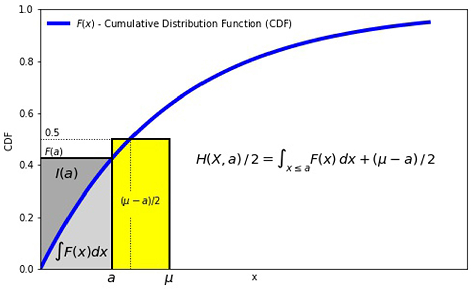
Figure 1. Geometric interpretation of H(X, a).

The MAD is twice the sum of two areas: the first area is the area under the cumulative distribution function for x ≤ a and the second area is (μ − a) · 0.5.

For MAD around the mean μ and the median M, we obtain

$\begin{array}{r}H(X,\mu )=2{\displaystyle {\int }_{x\le \mu }}F(x)dx\text{\hspace{1em} and}\\ H(X,M)=(\mu -M)+2{\displaystyle {\int }_{x\le M}}F(x)dx& (11)\end{array}$

2.2 MAD formula for discrete distributions

We now derive an analogous formula for the discrete distribution. Let Ω = {x₁, x₂, …}. Without loss of generality, assume x₁ < x₂ < ⋯ . By analogy with the continuous case, define the auxiliary sum I(x) as

$\begin{array}{ll}I(z)={\displaystyle \sum _{x_i\le z}}{x}_{i}f(x_i)& (12)\end{array}$

Then MAD of X from μ is

$\begin{array}{l}H(X,a)={\displaystyle \sum _{x_i\le a}(a-x_i)}f(x_i)+{\displaystyle \sum _{x_i>a}(x_i-a)}f(x_i)\\ =\left(a{\displaystyle \sum _{x_i\le a}f}(x_i)-{\displaystyle \sum _{x_i\le a}{x}_i}f(x_i)\right)\\ +\left({\displaystyle \sum _{x_i>a}{x}_i}f(x_i)-a{\displaystyle \sum _{x_i>a}f}(x_i)\right)\\ =(aF(a)-I(a))+{\displaystyle \left((\mu -I(a))-a(1-F(a)\right)}\\ =a\left(2F(a)-1\right)+\mu -2I(a)& (13)\end{array}$

To compute I(a), we use the following summation by parts formula (analogous to integration by parts) [24]. If U = {u₁, u₂, …, u_n} and V = {v₁, …, v_n} are two sequences and Δ is the forward difference operator, then

$\begin{array}{ll}{\displaystyle \sum _{k=m}^n}{u}_k\Delta v_k=(u_n{v}_{n+1}-u_m{v}_m)-{\displaystyle \sum _{k=m+1}^n}{v}_k\Delta u_k& (14)\end{array}$

To apply the formula, we let m = 1, v_k = x_k and u_k = F(x_k). Then we have

$\begin{array}{l}{\displaystyle \sum _{k=1}^n}F(x_k)\Delta x_k=\left(x_{n+1}F(x_n)-x_{1}F(x_1)\right)\end{array}$

$\begin{array}{ll}-{\displaystyle \sum _{k=2}^n}{x}_{k}f(x_k)=x_{n+1}F(x_n)-I(x_n)& (15)\end{array}$

If we choose $n(a)=arg{max}_{x_i\le a}\left\{x_i\right\}$ for a given a, then F(a) = F(x_n(a)) and we have

$\begin{array}{ll}I(a)=F(a)·x_{n(a)+1}-{\displaystyle \sum _{k=1}^n}\Delta x_{k}F(x_k)& (16)\end{array}$

in complete analogy for I(a) for the continuous case in Equation 9.

Substituting this expression for I(a) from Equation 16 into Equation 13, we obtain

$\begin{array}{ll}H(X,a)=(\mu -a)+2{\displaystyle \sum _{i\le n}}\Delta x_{i}F(x_i)& (17)\end{array}$

The sum on the right of Equation 17 is the area under the cumulative distribution function for x_i ≤ a and can be interpreted as the integral of the CDF computed for x ≤ a in direct analogy with the continuous case.

For MAD about mean μ and median M, the above equation gives us

$\begin{array}{r}H(X,\mu )=2{\displaystyle \sum _{x_i\le \mu }\Delta }{x}_{i}F(x_i)\text{\hspace{1em}\hspace{1em} and }\\ H(X,M))=(\mu -M)+2{\displaystyle \sum _{x_i\le M}\Delta }{x}_{i}F(x_i)& (18)\end{array}$

The advantage of these formulas is that for many distributions, x_i are consecutive integers, giving us Δx_i = 1. In such cases, the above formulas for H(X, μ) and H(X, M) simplify to

$\begin{array}{r}H(X,\mu )=2{\displaystyle \sum _{x_i\le \mu }}F(x_i)\text{\hspace{1em}and}\\ H(X,M)=(\mu -M)+2{\displaystyle \sum _{i\le M}}F(x_i)& (19)\end{array}$

with a direct analogy to the continuous case.

We will apply the above results to compute MADs of several well-known discrete distributions in Section 6.

3 Interpretation of MADs via “folded” cumulative distribution functions

We can interpret H(x, a) as follows. Consider the function G(x) defined as follows:

$\begin{array}{ll}G(x,a)=\{\begin{array}{ll}F(x)& x\in {\Omega }_L(a)\\ 1-F(x)& x\in {\Omega }_R(a)\\ 0& otherwise\end{array}& (20)\end{array}$

We can interpret G(x) as the "folded" cumulative distribution function curve. Note that unless F(a) = 1/2 (i.e., a is the median M), the curve G(x) is discontinuous at x = a. The case a = μ is illustrated in Figure 2.

Figure 2

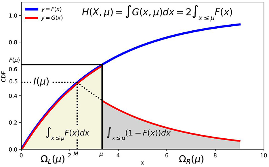
Figure 2. Illustration of folded cumulative distribution function (a = μ) and X ≥ 0.

For non-negative valued random variables X, we can interpret MAD H(X, a) in terms of G(x) as follows: let A(G) denote the area under this curve. For continuous case, we have

$\begin{array}{l}A(G)={\displaystyle {\int }_{\Omega }}G(x,a)dx={\displaystyle \underset{A_L}{{\displaystyle \underbrace{{\displaystyle {\int }_{{\Omega }_L(a)}}F(x)dx}}}}+{\displaystyle \underset{A_R}{{\displaystyle \underbrace{{\displaystyle {\int }_{{\Omega }_R(a)}}(1-F(x))dx}}}}\\ ={\displaystyle {\int }_{{\Omega }_L(a)}}\left[{\displaystyle {\int }_{y\le x}}dF(y)\right]dx+{\displaystyle {\int }_{{\Omega }_R(a)}}\left[{\displaystyle {\int }_{y>x}}dF(y)\right]dx\\ ={\displaystyle {\int }_{{\Omega }_L(a)}}\left[{\displaystyle {\int }_y^a}dx\right]dF(y)+{\displaystyle {\int }_{{\Omega }_R(a)}}\left[{\displaystyle {\int }_a^y}dx\right]dF(y)\\ ={\displaystyle {\int }_{{\Omega }_L(a)}}(a-y)dF(y)+{\displaystyle {\int }_{{\Omega }_R(a)}}(y-a)dF(y)\\ ={\displaystyle {\int }_{\Omega }}|a-y|dF(y)=H(X,a)\end{array}$

Comparing Equation 21 with Equation 8, we can interpret A_L = aF(a) − I(a) as the area under left part of G(x, a) for x ≤ a and A_R = (μ − I(a) − a(1 − F(a)) as the area under the right part of G(x, a) for x > a.

For the case a = μ, the areas under the curve for x ≤ a and x > a are equal. In this case, H(X, μ) = 2A_L(G) is just twice the area under the "left" part of the folded CDF curve for x ≤ a. This is illustrated in Figure 2. From Equation 9, the auxiliary integral I(μ) is the area above cumulative distribution function F(x) for x ≤ μ and F(x) ≤ F(μ) (shown in yellow color).

For the case a = M, the folded cumulative distribution function G(x) is continuous as shown in Figure 3. The area under this curve is the MAD from the median [25]. It is interesting to compare the MAD H(X, M) around the median with the quartile deviation (QD) defined as half of the interquartile range semi-interquartile range QD = IQR/2 = (Q₃ − Q₁)/2 where Q₁ and Q₃ are the first and third quartile of X. The MAD around the median is the area under the folded CDF G(x) where the quartile deviation is the area spanned between the quartiles on the x-axis and between 0 and 1/2 on the y-axis.

Figure 3

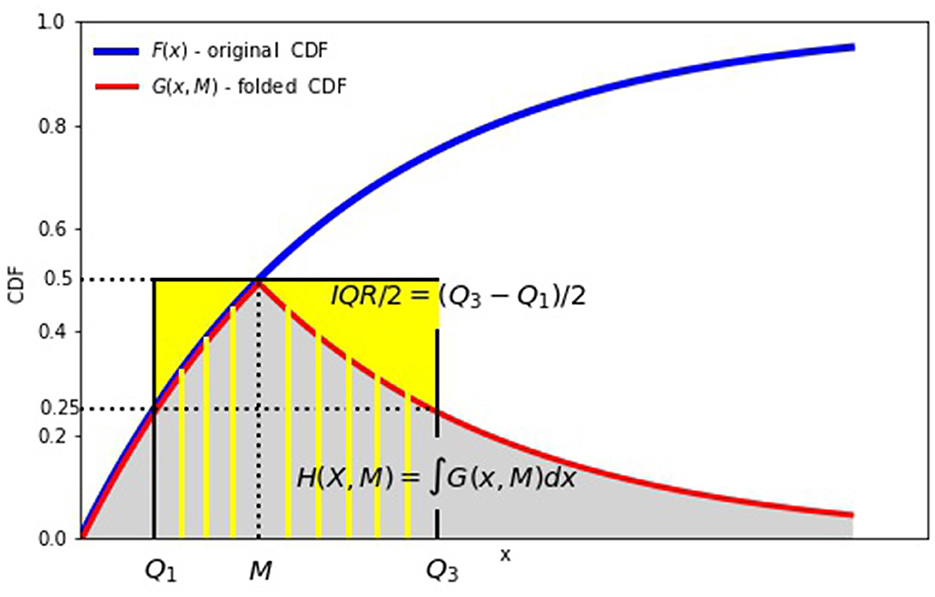
Figure 3. Mean absolute vs. quantile deviation (a = M and ≥ > 0.

For the discrete case with non-negative valued X, we get a similar result. As before we assume that 0 ≤ x₁ < x₂ < ⋯  and let $n(a)=arg{max}_{x_i\le a}\left\{x_i\right\}$. Recall that F(x_k) = f(x₁) + ⋯ + f(x_k). Therefore, we obtain

$\begin{array}{l}A(G)={\displaystyle \sum _i}\Delta x_{i-1}G(x_i,a)={\displaystyle \sum _{i\le n(a)}}\Delta x_{i-1}F(x_i)\\ +{\displaystyle \sum _{i>n(a)}}\Delta x_{i-1}(1-F(x_i))\\ ={\displaystyle \sum _{i\le n(a)}}\left((x_i-a)+(a-x_{i-1})\right)F(x_i)\\ +{\displaystyle \sum _{i>n(a)}}((a-x_{i-1})+(x_i-a))\left(1-F(x_i)\right)\\ ={\displaystyle \sum _{i\le a(n)}}(a-x_i)\Delta F(x_{i-1})+{\displaystyle \sum _{i>a(n)}}(x_i-a)\Delta F(x_{i-1})\\ ={\displaystyle \sum _{i\le a(n)}}(a-x_i)f(x_i)+{\displaystyle \sum _{i>a(n)}}(x_i-a)f(x_i)\\ ={\displaystyle \sum _i}|a-x_i|f(x_i)=H(X,a)\end{array}$

in exact analogy with the continuous case. Therefore, the MAD H(X, a) can also be interpreted as the area under the folded CDF curve G(x, a).

4 Some special functions and integrals

For many distributions, their cumulative distribution functions involve some special functions (for real arguments) such as Gamma and Beta functions [26, 27]. Indefinite integrals for many of these functions are readily available [28–30]. Some of these functions and their integrals are presented here for easy reference.

4.1 Some special functions and integrals

1. Error function ([30], Section 7.2 in Olver et al. [31]):

$\begin{array}{ll}\text{erf}(z)=\frac{2}{\sqrt{\pi }}{\displaystyle {\int }_0^z}{e}^{-t^2}dt& (21)\end{array}$

2. Density of the standard normal [31, 32]:

$\begin{array}{ll}\varphi (x)=\frac{1}{\sqrt{2\pi }}{e}^{-x^2/2}& (22)\end{array}$

3. Cumulative distribution of the standard normal [31, 32]:

$\begin{array}{ll}\Phi (x)=\frac{1}{\sqrt{2\pi }}{\displaystyle {\int }_{-\infty }^x}{e}^{-t^2/2}dt=\frac{1}{2}+\frac{1}{2}\text{erf}\left(\frac{x}{\sqrt{2}}\right)& (23)\end{array}$

4. Lower and upper incomplete Gamma functions ([30], Section 8.6 in Olver et al. [31]):

$\begin{array}{ll}\nu (s,x)={\displaystyle {\int }_0^x}{t}^{s-1}{e}^{-t}dt\text{\hspace{1em} and\hspace{1em} }\Gamma (s,x)={\displaystyle {\int }_x^{\infty }}{t}^{s-1}{e}^{-t}dt& (24)\end{array}$

5. Gamma function and regularized Gamma function ([30], Section 5.2 in Olver et al. [31]):

$\begin{array}{r}\Gamma (s)={\displaystyle {\int }_0^{\infty }}{t}^{s-1}{e}^{-t}dt=\nu (s,x)+\Gamma (s,x)\text{\hspace{1em}and}\\ Q(s,x)=\frac{\Gamma (s,x)}{\Gamma (s)}& (25)\end{array}$

6. Beta function (Section 5.12 in Olver et al. [31] and Gupta and Nadarajah [33]):

$\begin{array}{ll}B(z_1,z_2)={\displaystyle {\int }_0^1}{t}^{z_1-1}{(1-t)}^{z_2-1}dt=\frac{\Gamma (z_1)\Gamma (z_2)}{\Gamma (z_1+z_2)}& (26)\end{array}$

7. Incomplete Beta function and regularized incomplete Beta functions ([33], Section 8.17 in Olver et al. [31]):

$\begin{array}{r}B(x;a,b)={\displaystyle {\int }_0^x}{t}^{a-1}{(1-t)}^{b-1}dt\text{\hspace{1em}and}\\ I_x(a,b)=\frac{B(x;a,b)}{B(a,b)}& (27)\end{array}$

4.2 Some indefinite integrals

The following expressions will be used in many of the computations (C is a constant).

1. Integration of standard normal CDF (p. 396 in Owen [32]):

$\begin{array}{ll}{\displaystyle \int \Phi (a+bx)dx=\frac{(a+bx)\Phi (a+bx)+\varphi (a+bx)}{b}+C}& (28)\end{array}$

2. Integration of the product of standard normal density and x (integral #11, p. 393 in Owen [32]):

$\begin{array}{ll}{\displaystyle \int x\varphi (ax)dx=-\frac{\varphi (ax)}{a}+C}& (29)\end{array}$

3. Integration of the product of error function and exponential (integral #1, Section 4.2 in Ng and Geller [30]):

$\begin{array}{r}{\displaystyle \int e^{bx}\text{ erf}(az)dz=\frac{e^{bz}}{b}\text{ erf}(az)-\frac{1}{b}exp\left(\frac{b^2}{4a^2}\right)}\\ \text{erf}\left(az-\frac{b}{2a}\right)+C& (30)\end{array}$

4. Integration of incomplete gamma function (using integration by parts and Equation 24):

$\begin{array}{ll}{\displaystyle \int x^{b-1}\nu (\alpha ,z)dz=\frac{1}{b}\left(z^b\nu (\alpha ,z)-\nu (\alpha +b,z)\right)+C}& (31)\end{array}$

In particular, for b = 1 using the recurrence relation (chapter 8.6 in Olver et al. [31]),

$\nu (\alpha +1,z)=z\nu (s,z)-z^{\alpha }{e}^{-z}$

we obtain

$\begin{array}{ll}{\displaystyle \int \nu (\alpha ,z)dz=z^{\alpha }{e}^{-z}+C}& (32)\end{array}$

5. Integration of the incomplete beta function [33]

$\begin{array}{ll}{\displaystyle \int B(x;a,b)dx=xB(x;a,b)-B(x;a+1,b)+C}& (33)\end{array}$

6. Integration of reciprocal functions with exponentials (integral 2.313 p. 92 in Gradshteyn and Ryzhik [29])

$\begin{array}{ll}{\displaystyle \int \frac{dx}{a+b{e}^{mx}}=\frac{mx-log\left(1+b{e}^{mx}\right)}{am}+C}& (34)\end{array}$

5 MAD computations for continuous distributions

We now illustrate the above formula for some well-known continuous distributions. We will focus on MAD around the mean μ. We will consider the following continuous distributions (in alphabetical order): Beta, chi-squared, exponential, Gamma, Gumbel type I, half-normal, Laplace, logistic, Maxwell, normal, Pareto type I and II, Rayleigh, Student-t, triangular, uniform, and Weibull. For some of these distributions, the expressions for MAD have been known. In contrast, to our knowledge, the expressions for MAD have not been published for some distributions like Pareto II and Weibull.

1. Beta distribution with parameters α, β > 0: The corresponding density f(x) and the cumulative distribution function F(x) are given by Johnson and Kotz [20] and Feller [34]:

$\begin{array}{l}f(x)=\frac{x^{\alpha -1}{(1-x)}^{\beta -1}}{B(\alpha ,\beta )}\text{\hspace{1em}and\hspace{1em}}F(x)=I_x(\alpha ,\beta ),x\in (0,1)\end{array}$

where I_x(·) denotes the regularized incomplete beta function in Equation 27. The mean and standard deviation of this distribution are

$\begin{array}{l}\mu =\frac{\alpha }{\alpha +\beta }\text{\hspace{1em}and\hspace{1em}}\sigma =\frac{1}{\alpha +\beta }\sqrt{\frac{\alpha \beta }{\alpha +\beta +1}}\end{array}$

Therefore, using Equation 33 we compute H(X, μ) as follows:

$\begin{array}{l}H(X,\mu )=2{\displaystyle {\int }_0^{\mu }}{I}_x(\alpha ,\beta )dx\\ {\displaystyle =\frac{2xB(x;\alpha ,\beta )-2B(x;\alpha +1,\beta )}{B(\alpha ,\beta )}{|}_0^{\mu }}\\ =\frac{2\mu B(\mu ;\alpha ,\beta )-2B(\mu ;\alpha +1,\beta )}{B(\alpha ,\beta )}& (35)\end{array}$

There is no closed-form formula for the median M. The MAD around the median M is

$\begin{array}{l}H(X,M)=(\mu -M)+2{\displaystyle {\int }_0^M}{I}_x(\alpha ,\beta )dx=\left(\frac{\alpha }{\alpha +\beta }-M\right)\\ +\frac{2M·B(M;\alpha ,\beta )-2B(M;\alpha +1,\beta )}{B(\alpha ,\beta )}& (36)\end{array}$

2. Exponential distribution with rate λ > 0 : The corresponding density f(x) and cumulative distribution function F(x) are given by Johnson and Kotz [20] and Feller [34]:

$\begin{array}{l}f(x)=\lambda e^{-\lambda x}\text{\hspace{1em} and\hspace{1em} }F(x)=1-e^{-\lambda x},x\ge 0\end{array}$

Its mean μ = 1/λ and standard deviation σ = 1/λ. We compute H(X, μ) as

$\begin{array}{r}{\displaystyle H(X,\mu )=2{\displaystyle {\int }_0^{1/\lambda }}(1-e^{-\lambda x})dx=2\left(x+\frac{e^{-\lambda x}}{\lambda }\right){|}_0^{1/\lambda }}\\ =\frac{2}{\lambda e}=\left(\frac{2}{e}\right)\sigma & (37)\end{array}$

In terms of σ, for this distribution H(X, μ) = (2/e)σ ≈ 0.74σ.

The median is M = (log2)/λ. The MAD about median is then

$\begin{array}{l}H(X,M)=(\mu -M)+2{\displaystyle {\int }_0^{log2/\lambda }}(1-e^{-\lambda x})dx\\ {\displaystyle =\left(\frac{1}{\lambda }-\frac{log2}{\lambda }\right)+2\left(x+\frac{e^{-\lambda x}}{\lambda }\right){|}_0^{log2/\lambda }=\frac{log2}{\lambda }}& (38)\end{array}$

3. F (Fisher–Snedecor) distribution with α, β > 0 degrees of freedom: The corresponding density f(x) and cumulative distribution function F(x) are given by Johnson and Kotz [20] and Feller [34],

$\begin{array}{r}f(x\alpha ,\beta )=\frac{\sqrt{\frac{{(\alpha x)}^{\alpha }{\beta }^{\beta }}{{(\alpha x+\beta )}^{\alpha +\beta }}}}{xB\left(\frac{\alpha }{2},\frac{\beta }{2}\right)}\text{\hspace{1em}and\hspace{1em}}F(x)=I_z\left(\frac{\alpha }{2},\frac{\beta }{2}\right),\\ \text{where}\{\begin{array}{l}z=\frac{\alpha x}{/(\alpha x+\beta )}\\ x>0,& \text{if }\alpha =1\\ x\ge 0& \text{if }\alpha >0\end{array}\end{array}$

The mean μ and standard deviation σ are defined only for β > 2 and β > 5 respectively and are given by

$\begin{array}{r}\mu =\frac{\beta }{\beta -2},\text{\hspace{1em}for }\beta >2\text{\hspace{1em}and}\\ \sigma =\frac{\beta }{(\beta -2)}\sqrt{\frac{2(\alpha +\beta -2)}{\alpha (\beta -4)}},\text{\hspace{1em}for }\beta >4\end{array}$

To compute H(X, μ) we note that x = βz/(α(1 − z)) and therefore, dz = (β/α(1 − z)²)dz. Let μ^* = αμ/(αμ + β) = α/(α + β − 2β). Therefore, for the MAD, we obtain

$\begin{array}{l}H(X,\mu )=2{\displaystyle {\int }_0^{\mu }}F(x)dx=\frac{2\beta }{\alpha }{\displaystyle {\int }_0^{{\mu }^{*}}}\frac{I_z(\alpha /2,\beta /2)}{{(1-z)}^2}dz\\ =\frac{2\beta }{\alpha B(\alpha /2,\beta /2)}\left[{\displaystyle {\int }_0^{{\mu }^{*}}}\frac{B(z;\alpha /2,\beta /2)}{{(1-z)}^2}dz\right]\end{array}$

To compute the integral, we note that B′(z; α/2, β/2) = z^{α/2 − 1}(1 − z)^{β/2 − 1}. If we consider the function h(z) = B(z; α/2, β/2)/(1 − z) then

$\begin{array}{l}{h}^{\prime }(z)=\frac{B^{\prime }(z;\alpha /2,\beta /2)}{(1-z)}+\frac{B(z;\alpha /2,\beta /2)}{{(1-z)}^2}\\ =z^{\alpha /2}{(1-z)}^{\beta /2-1}+\frac{B(z;\alpha /2,\beta /2)}{{(1-z)}^2}\end{array}$

This immediately gives us the expression for the integral

$\begin{array}{l}{\displaystyle \int \frac{B(z;\alpha /2,\beta /2)}{{(1-z)}^2}dz=\frac{B(z;\alpha /2,\beta /2)}{(1-z)}}\\ -B(z;\alpha /2,\beta /2-1)\end{array}$

We can now compute the MAD for the F distribution:

$\begin{array}{l}H(X,\mu )\\ {\displaystyle =\frac{2\beta }{\alpha B(\alpha /2,\beta /2)}\left[\frac{B(z;\alpha /2,\beta /2)}{(1-z)}-B(z;\alpha /2,\beta /2-1)\right]{|}_0^{{\mu }^{*}}}\\ =\frac{2\beta }{\alpha B(\alpha /2,\beta /2)}\left[\frac{B({\mu }^{*};\alpha /2,\beta /2)}{(1-{\mu }^{*})}-B({\mu }^{*};\alpha /2,\beta /2-1)\right]& (39)\end{array}$

4. Gamma distribution with shape parameter α > 0 and rate β > 0: The corresponding density f(x) and cumulative distribution function F(x) are given by Johnson and Kotz [20] and Feller [34]:

$\begin{array}{l}f(x)=\frac{{\beta }^{\alpha }{x}^{\alpha -1}{e}^{-\beta x}}{\Gamma (\alpha )}\text{\hspace{1em} and\hspace{1em} }F(x)=\frac{\nu (\alpha ,\beta x)}{\Gamma (\alpha )},x\ge 0\end{array}$

where Γ(·) denotes the Gamma function (Equation 25 and ν(·) denotes the lower incomplete Gamma function (Equation 24). The mean of this distribution is μ = α/β and its standard deviation $\sigma =\sqrt{\alpha }/\beta$.

Let us define z = βx. Then we have

$\begin{array}{l}H(X,\mu )=\frac{2}{\Gamma (\alpha )}{\displaystyle {\int }_0^{\mu }}\nu (\alpha ,\beta x)dx=\frac{2\beta }{\Gamma (\alpha )}{\displaystyle {\int }_0^{\alpha }}\nu (\alpha ,z)dz\\ {\displaystyle =\frac{2\beta }{\Gamma (\alpha )}[z^{\alpha }{e}^{-z}]{|}_0^{\alpha }}=\frac{2\beta {\alpha }^{\alpha }{e}^{-\alpha }}{\Gamma (\alpha )}& (40)\end{array}$

There is no closed-form expression for the median M. The MAD (around median) is

$\begin{array}{l}H(X,M)=(\mu -M)+2{\displaystyle {\int }_{x\le M}}F(x)dx=\left(\frac{\alpha }{\beta }-M\right)\\ +\frac{2\beta }{\Gamma (\alpha )}{\displaystyle {\int }_0^{\beta M}}\nu (\alpha ,\beta x)d(\beta x)\\ =\left(\frac{\alpha }{\beta }-M\right){\displaystyle +\frac{2\beta }{\Gamma (\alpha )}[z^{\alpha }{e}^{-z}]{|}_0^{\beta M}}=\left(\frac{\alpha }{\beta }-M\right)\\ +\frac{2\beta {(\beta M)}^{\alpha }}{\Gamma (\alpha )}{e}^{-\beta M}& (41)\end{array}$

5. χ² Distribution with k degrees of freedom: The corresponding density f(x) and the cumulative distribution function F(x) are given by Johnson and Kotz [20] and Feller [34]:

$\begin{array}{l}f(x)=\frac{x^{k/2-1}{e}^{-x/2}}{2^{k/2}\Gamma (k/2)}\text{\hspace{1em} and\hspace{1em} }F(x)=\frac{\nu (k/2,x/2)}{\Gamma (k/2)},x>0\end{array}$

where Γ(·) denotes the Gamma function (Equation 25 and ν(·) denotes the lower incomplete Gamma function (Equation 24. The mean of this distribution is μ = k and its standard deviation $\sigma =\sqrt{2k}$. This is a special case of Gamma distribution with shape α = k/2 and rate β = 1/2. This immediately gives us

$\begin{array}{r}H(X,\mu )=\frac{{(2e)}^{-k/2}{k}^{k/2}}{\Gamma (k/2)}\text{\hspace{1em}and}\\ H(X,M)=(k-M)+\frac{{(M/2)}^{k/2}{e}^{-M/2}}{\Gamma (k/2)}& (42)\end{array}$

6. Gumbel type I (extreme value distribution) with location μ and scale β > 0: The corresponding density and f(x) and cumulative distribution function F(x) are given by [20]):

$\begin{array}{l}f(x)=\frac{1}{\beta }{e}^{-(z+e^{-z})}\text{\hspace{1em}and\hspace{1em}}F(x)=e^{-e^{-z}},x\in R,z=(x-\mu )/\beta \end{array}$

Its mean is μ^* = (μ + βγ) where γ is the Euler-Mascheroni constant. Its standard deviation $\sigma =\beta \pi /\sqrt{6}$. Let t = e^−z. Then dt = (t/β)dx or dx = βt⁻¹dt. Then for MAD (about mean) we obtain

$\begin{array}{r}H(X,{\mu }^{*})=2{\displaystyle {\int }_{x\le {\mu }^{*}}}F(x)dx=2\beta {\displaystyle {\int }_0^{e^{-\gamma }}}{e}^{-t}{t}^{-1}dt\\ =2\beta \nu (0,e^{-\gamma })& (43)\end{array}$

where ν(·) denotes the incomplete lower gamma function in Equation 24.

The median for this distribution is M = μ − β log(log2). Therefore, for the MAD about the median we have

$\begin{array}{l}H(X,M)=({\mu }^{*}-M)+2{\displaystyle {\int }_{x\le M}}F(x)dx=\beta \left(\gamma +log(log2)\right)\\ +2\beta {\displaystyle {\int }_0^{log2}}{e}^{-z}{z}^{-1}dz\\ =\beta \left[\gamma +log(log2)+2\nu (0,log2)\right]& (44)\end{array}$

7. Half-normal distribution with scale parameter σ > 0: The corresponding density f(x) and cumulative distribution function F(x are given by Johnson and Kotz [20]):

$\begin{array}{l}f(x)=\frac{\sqrt{2}}{\sigma \sqrt{\pi }}{e}^{-x^2/(2{\sigma }^2)},\text{\hspace{1em}and\hspace{1em}}F(x)=\text{erf}\left(\frac{x}{\sigma \sqrt{2}}\right).x\ge 0\end{array}$

The mean is $\mu =\sigma \sqrt{2/\pi }$ and standard deviation ${\sigma }^{*}=\sigma (1-\sqrt{2/\pi })$. Let $z=x/(\sigma \sqrt{2})$. Then $dx=\sigma \sqrt{2}dz$ and we have

$\begin{array}{l}H(X,\mu )=2\sigma \sqrt{2}{\displaystyle {\int }_0^{1/\sqrt{\pi }}}\text{erf}(z)dz\\ {\displaystyle =2\sigma \sqrt{2}\left[z\text{ erf}(z)+\frac{1}{\sqrt{\pi }}{e}^{-z^2}\right]{|}_0^{1/\sqrt{\pi }}}\\ =2\sigma \sqrt{\frac{2}{\pi }}\left[\text{erf}\left(\frac{1}{\sqrt{\pi }}\right)+e^{-1/\pi }-1\right]& (45)\end{array}$

The median is $M=\sigma \sqrt{2}{\text{erf}}^{-1}(1/2)$. Define c = erf⁻¹(1/2). Then the MAD around the median M we have

$\begin{array}{l}H(X,M)=(M-\mu )+2\sigma \sqrt{2}{\int }_0^c\text{erf}(z)dz\\ {\displaystyle =\sigma \sqrt{2}\left(\frac{1}{\sqrt{\pi }}-c\right)+2\sigma \sqrt{2}\left[z\text{ erf}(z)+\frac{1}{\sqrt{\pi }}{e}^{-z^2}\right]{|}_0^c}\\ =\frac{\sigma \sqrt{2}}{\pi }\left(2e^{-c^2}-1\right)& (46)\end{array}$

8. Laplace distribution with location μ and scale b: The density f(x) and cumulative distribution function F(x) are given by Johnson and Kotz [20] and Feller [34]:

$\begin{array}{ll}f(x)=\frac{1}{2b}{e}^{-|x-\mu |/b}\text{ and}& F(x)=\{\begin{array}{l}\frac{1}{2}{e}^{(x-\mu )/b},\text{if }x\le \mu \\ 1-\frac{1}{2}{e}^{-(x-\mu )/b},\text{if }x\ge \mu \end{array}\end{array}$

For this distribution, μ = M = b and $\sigma =b\sqrt{2}$. For the MAD, we obtain

$\begin{array}{ll}{\displaystyle H(X,\mu )=H(X,M)={\displaystyle {\int }_{\infty }^{\mu }}{e}^{(x-\mu )/b}dx=b{e}^{(x-\mu )/b}{|}_{-\infty }^{\mu }=b}& (47)\end{array}$

In terms of σ, we have $H(X,\mu )=\sigma \sqrt{2}/2\approx 0.71\sigma$.

9. Logistic distribution with location μ and scale s > 0: The corresponding density function f(x) and cumulative distribution function F(x are given by Johnson and Kotz [20]:

$\begin{array}{l}f(x)=-\frac{e^{-(x-\mu )/s}}{s{(1+e^{-(x-\mu )/s})}^2},\text{\hspace{1em}and\hspace{1em}}F(x)=\frac{1}{1+e^{-(x-\mu )/s}},x\in R\end{array}$

The mean and the median are μ and the standard deviation is $\sigma =s\pi /\sqrt{3}$. Let z = (x − μ)/s. Since for this distribution M = μ, we have H(X, μ) = H(X, M). Using Equation 34 we obtain

$\begin{array}{l}H(X,\mu )=H(X,M)=2{\displaystyle {\int }_{-\infty }^{\mu }\frac{dx}{1+e^{-(x-\mu )/s}}}=2{\displaystyle {\int }_{-\infty }^0\frac{zdz}{1+e^{-z}}}\\ ={2s\left[z+\text{log}(1+e^{-z})\right]|}_{-\infty }^0\\ {\displaystyle ={2s\left[z+\log \left(e^{-z}(e^z+1)\right)\right]|}_{-\infty }^0}\\ {\displaystyle ={2s\log (e^z+1)|}_{-\infty }^0=2s\log 2}& (48)\end{array}$

In terms of σ we have $H(X,\mu )=(2\sqrt{3}log2/\pi )\sigma \approx 0.76\sigma$

10. Log-normal distribution with parameters μ ∈ (∞, +∞) and σ² (σ > 0): The density f(x) and cumulative distribution function F(x) are given by Johnson and Kotz [20] and Feller [34]:

$\begin{array}{r}f(x)=\frac{1}{x\sigma \sqrt{2\pi }}{e}^{-{(logx-\mu )}^2/2{\sigma }^2}=x\sigma \varphi \left(\frac{logx-\mu }{\sigma }\right),\text{ and}\\ F(x)=\Phi \left(\frac{logx-\mu }{\sigma }\right),x>0\end{array}$

We will use the notation μ^* and σ^* to denote the mean and standard deviation of X to distinguish it from the mean μ and standard deviation σ of the underlying normal distribution. The mean of the log-normal distribution is μ^* = e^μ+σ2/2 and its standard deviation ${\sigma }^{*}=e^{\mu +{\sigma }^2/2}\sqrt{e^{{\sigma }^2}-1}$.

To compute H(X, μ), define z = (log x − μ)/σ. Then, dx = σx dz = σe^{μ + σz}dz and using Equation 30 with $a=1/\sqrt{2}$ and b = σ, we obtain

$\begin{array}{l}H(X,{\mu }^{*})=2{\displaystyle {\int }_0^{{\mu }^{*}}}\Phi \left(\frac{logx-\mu }{\sigma }\right)dx=2\sigma e^{\mu }{\displaystyle {\int }_{-\infty }^{\sigma /2}}{e}^{\sigma z}\Phi (z)dz\\ =2\sigma e^{\mu }{\displaystyle {\int }_{-\infty }^{\sigma /2}}{e}^{\sigma z}\left[\frac{1}{2}+\frac{1}{2}\text{ erf}\left(\frac{z}{\sqrt{2}}\right)\right]dz\\ =2e^{\mu +{\sigma }^2/2}\text{ erf}\left(\frac{\sigma }{2\sqrt{2}}\right)& (49)\end{array}$

The median M = e^μ and therefore for the MAD around median, we obtain

$\begin{array}{l}H(X,M)=({\mu }^{*}-M)+2{\displaystyle {\int }_0^M}\Phi \left(\frac{logx-\mu }{\sigma }\right)dx\\ =e^{\mu }(e^{{\sigma }^2/2}-1)+2\sigma e^{\mu }{\displaystyle {\int }_{-\infty }^0}{e}^{\sigma z}\Phi (z)dz\\ =e^{\mu }(e^{{\sigma }^2/2}-1)+2\sigma e^{\mu }{\displaystyle {\int }_{-\infty }^0}{e}^{\sigma z}\left[\frac{1}{2}+\frac{1}{2}\text{ erf}\left(\frac{z}{\sqrt{2}}\right)\right]dz\\ =e^{\mu +{\sigma }^2/2}+\sigma e^{\mu }{\displaystyle {\int }_{-\infty }^0}{e}^{\sigma z}\text{ erf}\left(\frac{z}{\sqrt{2}}\right)dz\\ =e^{\mu +{\sigma }^2/2}\text{ erf}\left(\frac{\sigma }{\sqrt{2}}\right)& (50)\end{array}$

11. Maxwell (or Maxwell-Boltzmann) distribution with scale parameter b > 0: The density function f(x) and the cumulative distribution function F(x) are given by Johnson and Kotz [20]

$\begin{array}{r}f(x)=\frac{1}{b^3}\sqrt{\frac{2}{\pi }}{x}^2{e}^{-x^2/{(2b)}^2}\text{\hspace{1em} and}\\ F(x)=2\Phi \left(\frac{x}{b}\right)-\frac{1}{b}\sqrt{\frac{2}{\pi }}x{e}^{-x^2/{(2b)}^2}x\ge 0\end{array}$

We can re-write these as

$\begin{array}{r}f(x)=2{\left(\frac{x}{b}\right)}^2\varphi \left(\frac{x}{b}\right)\text{\hspace{1em}and}\\ F(x)=2\Phi \left(\frac{x}{b}\right)-2\left(\frac{x}{b}\right)\varphi \left(\frac{x}{b}\right)x\ge 0\end{array}$

The mean is $\mu =2b\sqrt{2/\pi }$ and standard deviation $\sigma =b\sqrt{(3\pi -8)/\pi }$. We let z = x/b. Then dx = b dz and using Equations 28, 29, with a = 1/b, we obtain

$\begin{array}{l}H(X,\mu )=4b{\displaystyle {\int }_0^{2\sqrt{2}}}\left(\Phi (z)-z\varphi (z)\right)dz\\ {\displaystyle =4b\left(z\Phi (z)+2\varphi (z)\right){|}_0^{2\sqrt{2}/\sqrt{\pi }}}\\ =4b\sqrt{\frac{2}{\pi }}\left(\text{erf}\left(\frac{2}{\sqrt{\pi }}\right)+e^{-\pi /4}\right)& (51)\end{array}$

There is no simple closed-form for the median M.

12. Normal distribution N(μ, σ): The density f(x) and cumulative distribution function F(x) are [20, 34]:

$\begin{array}{l}f(x)=\frac{1}{\sigma }\varphi \left(\frac{x-\mu }{\sigma }\right)\text{\hspace{1em}and\hspace{1em}}F(x)=\Phi \left(\frac{x-\mu }{\sigma }\right),x\in R\end{array}$

where Φ(·) denotes the cumulative distribution of the standard normal (Equation 23). Using Equation 28 with a = −μ/σ and b = 1/σ we obtain

$\begin{array}{l}H(X,\mu )=2{\int }_{x\le \mu }\Phi \left(\frac{x-\mu }{\sigma }\right)\\ dx=2\sigma {\left(x\Phi (x)+f(x)\right)|}_{-\infty }^0=\sigma \sqrt{\frac{2}{\pi }}& (52)\end{array}$

In terms of σ, we have $H(X,\mu )=\sigma \sqrt{2/\pi }\approx 0.80\sigma$. Since this is a symmetric distribution H(X, M) = H(X, μ).

13. Pareto type I distribution with shape α > 0 and scale β > 0: The density f(x) and the cumulative distribution function F(x) are given by Johnson and Kotz [20]

$\begin{array}{l}f(x)=\{\begin{array}{l}\frac{\alpha {\beta }^{\alpha }}{x^{\alpha +1}}x\ge \beta \\ 0x<\beta \end{array}\text{ and }F(x)=\{\begin{array}{l}1-{\left(\frac{\beta }{x}\right)}^{\alpha }x\ge \beta \\ 0x<\beta \end{array}\end{array}$

the mean and standard deviation for this distribution are

$\begin{array}{r}\mu =\frac{\alpha \beta }{(\alpha -1)}\text{\hspace{1em}if\hspace{1em}}\alpha >1\text{\hspace{1em}and}\\ \sigma =\frac{\beta }{(\alpha -1)}\sqrt{\frac{\alpha }{(\alpha -2)}}\text{ if\hspace{1em}}\alpha >2\end{array}$

This distribution has infinite mean μ for α ≤ 1 and infinite variance for α ≤ 2. We assume that α > 1. Then for MAD, we obtain

$\begin{array}{l}{\displaystyle H(X,\mu )=2{\displaystyle {\int }_{\beta }^{\mu }}\left(1-{\left(\frac{\beta }{x}\right)}^{\alpha }\right)dx=2\left[x+\frac{{\beta }^{\alpha }}{(\alpha -1)}{x}^{-\alpha +1}\right]{|}_{\beta }^{\mu }}\\ =2\left[\frac{\alpha \beta }{(\alpha -1)}+\frac{{\beta }^{\alpha }}{(\alpha -1)}{\left(\frac{\alpha \beta }{\alpha -1}\right)}^{-\alpha +1}\right]\\ -2\left[\beta +\frac{{\beta }^{\alpha }}{(\alpha -1)}{\beta }^{-\alpha +1}\right]\\ =\frac{2\beta }{\alpha }{\left(1-\frac{1}{\alpha }\right)}^{\alpha -2}& (53)\end{array}$

The median is $M=\beta \sqrt[\alpha ]{2}$. Therefore, for the MAD about the median, we obtain

$\begin{array}{l}H(X,M)=(\mu -M)+2{\displaystyle {\int }_{\beta }^M}\left(1-{\left(\frac{\beta }{x}\right)}^{\alpha }\right)dx\\ {\displaystyle =\left(\frac{\alpha \beta }{(\alpha -1)}-\beta \sqrt[\alpha ]{2}\right)+2\left[x+\frac{{\beta }^{\alpha }}{(\alpha -1)}{x}^{-\alpha +1}\right]{|}_{\beta }^M}\\ {\displaystyle =\left(\frac{\alpha \beta }{(\alpha -1)}+\beta \sqrt[\alpha ]{2}\right)+2\left[\frac{{\beta }^{\alpha }}{(\alpha -1)}{x}^{-\alpha +1}\right]{|}_{\beta }^{\beta \sqrt[\alpha ]{2}}}\\ =\frac{\alpha \beta \left(\sqrt[\alpha ]{2}-1\right)}{(\alpha -1)}& (54)\end{array}$

14. Generalized Pareto (Type II) distribution with location μ ∈ R, scale σ > 0, and shape ξ ∈ R: We exclude the case ξ = μ = 0, that corresponds to the exponential distribution. The density f(x) and the cumulative distribution function F(x) are given by Johnson and Kotz [20]:

$\begin{array}{r}f(x)=\{\begin{array}{ll}\frac{1}{\sigma }{\left(1+\frac{\xi (x-\mu )}{\sigma }\right)}^{-1/\xi -1}& \xi \ne 0\\ exp\left(-\frac{(x-\mu )}{\sigma }\right)& \xi =0\end{array}\text{\hspace{1em}and}\\ F(x)=\{\begin{array}{ll}1-{\left(1+\frac{\xi (x-\mu )}{\sigma }\right)}^{-1/\xi }& \xi \ne 0\\ 1-exp\left(-\frac{(x-\mu )}{\sigma }\right)& \xi =0\end{array}\end{array}$

where the support of X is x ≥ μ for ξ ≥ 0 and μ ≤ x ≤ σ/ξ for ξ < 0. The mean μ^* and standard deviation σ^* of this distribution are defined only for ξ < 1 and ξ < 1/2 respectively and are

$\begin{array}{r}{\mu }^{*}=\mu +\frac{\sigma }{(1-\xi )},\xi <1\text{\hspace{1em}and}\\ {\sigma }^{*}=\frac{\sigma }{(1-\xi )\sqrt{1-2\xi }},\xi <1/2\end{array}$

To compute H(X, μ^*), we need to consider two cases

(a) ξ < 1 and ξ ≠ 0. We have

$\begin{array}{l}H(X,{\mu }^{*})=2{\displaystyle {\int }_{\mu }^{{\mu }^{*}}}F(x)dx\\ {\displaystyle =\left[x+\frac{\sigma }{1-\xi }{\left(1+\frac{\xi (x-\mu )}{\sigma }\right)}^{1-1/\xi }\right]{|}_{\mu }^{{\mu }^{*}}}\\ =2\left[\mu +\frac{\sigma }{1-\xi }+\sigma {\left(\frac{1}{1-\xi }\right)}^{2-1/\xi }\right]\\ -2\left[\mu +\frac{\sigma }{1-\xi }\right]=2\sigma {\left(\frac{1}{1-\xi }\right)}^{2-1/\xi }& (55)\end{array}$

Note that the case ξ = −1 gives H(X, μ^*) = σ/4 and corresponds to continuous uniform distribution U(0, σ). The case ξ > 0 and location μ = σ/ξ corresponds to the Pareto distribution with scale β = σ/ξ and shape α = 1/ξ.

(b) Case ξ = 0. For this case, we obtain

$\begin{array}{l}H(X,{\mu }^{*})=2{\displaystyle {\int }_{x=\mu }^{{\mu }^{*}}}F(x)dx\\ {\displaystyle =2\left[x+\sigma exp\left(-\frac{(x-\mu )}{\sigma }\right)\right]{|}_{\mu }^{{\mu }^{*}}}\\ =2\left[\mu +\frac{\sigma }{1-\xi }-\frac{\sigma }{exp(1-\xi )}\right]-2\left[\mu +\frac{\sigma }{e}\right]\\ =2\sigma \left[\frac{1}{1-\xi }-\frac{1}{exp(1-\xi )}+\frac{1}{e}\right]\end{array}$

Note that for ξ = 0, the case μ = 0 corresponds to an exponential distribution with parameter 1/σ.

For μ = 0 and ξ > 0, let α = 1/ξ and λ = ξσ. Then we obtain the Lomax distribution with shape α > 0 and scale λ > 0. Its mean μ^* = λ/(α − 1) is defined only for α > 1 (corresponding to ξ < 1). Therefore, for α > 1 its MAD for the Lomax distribution is

$\begin{array}{l}H(X,{\mu }^{*})=2\lambda \alpha {\left(\frac{\alpha }{\alpha -1}\right)}^{2-\alpha }\end{array}$

15. Rayleigh distribution with scale parameter σ > 0: The density function f(x) and the cumulative distribution function F(x) are given by Johnson and Kotz [20]:

$\begin{array}{l}f(x)=-\frac{x}{{\sigma }^2}{e}^{-x^2/{(2\sigma )}^2},\text{\hspace{1em}and\hspace{1em}}F(x)=1-e^{-x^2/{(2\sigma )}^2},x\ge 0\end{array}$

The mean is $\mu =\sigma \sqrt{\pi /2}$ and standard deviation is ${\sigma }^{*}=\sigma \sqrt{(4-\pi )/2}$. Let z = x/2σ. Then dx = 2σ dz and we have

$\begin{array}{l}H(X,\mu )=2\sigma \sqrt{\frac{\pi }{2}}-4\sigma {\displaystyle {\int }_0^{\sqrt{\pi }/2\sqrt{2}}}{e}^{-z^2}dz\\ =2\sigma \sqrt{\pi }\left(\frac{\sqrt{2}}{2}-\text{erf}\left(\frac{\sqrt{\pi }}{2\sqrt{2}}\right)\right)& (56)\end{array}$

For this distribution, the median $M=\sigma \sqrt{2log2}$. Therefore,

$\begin{array}{l}H(X,M)=(\mu -M)+2{\displaystyle {\int }_{x\le M}(1-e^{-x^2/{(2\sigma )}^2})}dx\\ =\sigma \left(\sqrt{\pi /2}-\sqrt{2\text{ log }2}\right)+2\sigma \sqrt{2\text{ log }2}\\ -4\sigma {\displaystyle {\int }_0^{\sqrt{(\text{log }2)/2}}{e}^{-z^2}}dz\\ =\sigma \left[\sqrt{\pi /2}+\sqrt{2\text{ log }2})-2\sqrt{\pi }\text{ erf}\left(\sqrt{\frac{\text{log }2}{2}}\right)\right]& (57)\end{array}$

16. Student-t distribution with k > 1 degrees of freedom: Its probability density function f(x) and its cumulative distribution function F(x) are given by Johnson and Kotz [20] and Feller [34]:

$\begin{array}{r}f(x)=\frac{1}{\sqrt{k}B(k/2,1/2)}{\left(1+\frac{x^2}{k}\right)}^{-(k+1)/2}\text{\hspace{1em}and}\\ F(x)=1-\frac{B(1/(1+x^2/k),k/2,1/2)}{2B(k/2,1/2)},x\in R\end{array}$

The mean μ is μ = 0 for k > 1, otherwise it is undefined. The standard deviation is defined only for k > 2 and σ = k/(k − 2). From Equation 8 we have

$\begin{array}{l}H(X,\mu )=-2{\displaystyle {\int }_{-\infty }^0}xf(x)dx\\ =-\frac{2}{\sqrt{k}B\left(1/2,k/2\right)}{\displaystyle {\int }_{-\infty }^0}x{\left(1+\frac{x^2}{k}\right)}^{-(k+1)/2}dx\\ {\displaystyle =-\frac{2}{\sqrt{k}B(1/2,k/2)}\left[-\frac{k}{2(k-1)}{\left(1+\frac{x^2}{k}\right)}^{-(k-1)/2}\right]{|}_{-\infty }^0}\\ =\frac{\sqrt{k}}{(k-1)B(k/2,1/2)}& (58)\end{array}$

Since this distribution is symmetric, M = μ and H(X, M) = H(X, μ).

17. Triangular distribution with lower limit a, upper limit b and mode c ∈ [0, 1]: The density function f(x) and the cumulative distribution function F(x) is given by [20, 34, 35]:

$\begin{array}{l}f(x)=\{\begin{array}{l}\frac{2(x-a)}{(b-a)(c-a)}\\ \frac{2(b-x)}{(b-a)(b-c}\end{array}F(x)=\{\begin{array}{ll}\frac{{(x-a)}^2}{(b-a)(c-a)}& \text{for\hspace{0.17em}}0\le x\le c,\\ 1-\frac{{(b-x)}^2}{(b-a)(b-c)}& \text{for\hspace{0.17em}}c<x\le 1\end{array}\end{array}$

For this distribution, μ = (a + b + c)/3 and $\sigma =\sqrt{{(b-a)}^2-(c-a)(b-c)}/3\sqrt{2}$. It is easy to show that for 0 ≤ c ≤ (a + b)/2, we have μ ≥ c and for (a + b)/2 ≤ c ≤ b, we have μ ≤ c. Therefore,

$\begin{array}{l}H(X,\mu )=2{\int }_{x\le \mu }F(x)dx\\ =\{\begin{array}{ll}\frac{2}{3(b-a)(b-c)}{\left(\frac{2b-(a+c)}{3}\right)}^3& \text{for }0\le c\le (a+b)/2\\ \frac{2}{3(b-a)(c-a)}{\left(\frac{b+c-2a}{3}\right)}^3& \text{for }(a+b)/2\le c\le \end{array}\end{array}$

The median M of this distribution is

$\begin{array}{ll}M=\{\begin{array}{cc}b-\frac{\sqrt{2}}{2}\sqrt{(b-a)(b-c)}& c\le (a+b)/2\\ a+\frac{\sqrt{2}}{2}\sqrt{(b-a)(c-a)}& c\ge (a+b)/2\end{array}& (59)\end{array}$

Therefore, the MAD about the median is then

$\begin{array}{l}H(X,M)=(\mu -M)+{\displaystyle {\int }_{x\le M}}F(x)dx\\ =\{\begin{array}{cc}\frac{(b-a)+(b-c)-\sqrt{2(b-a)(b-c)}}{3}& a\le c\le (a+b)/2\\ \frac{(b-a)+(c-a)-\sqrt{2(b-a)(c-a)}}{3}& (a+b)/2\le c\le b\end{array}& (60)\end{array}$

18. Uniform continuous distribution in [a, b]: The density function f(x) and the cumulative distribution function F(x) are given by Johnson and Kotz [20] and Feller [34]:

$\begin{array}{l}f(x)=\frac{1}{(b-a)}\text{\hspace{1em}and\hspace{1em}}F(x)=\frac{(x-a)}{(b-a)}x\in \left[a,b\right]\end{array}$

Mean is μ = (a + b)/2 and standard deviation $\sigma =(b-a)/2\sqrt{3}$. The MAD is

$\begin{array}{l}{\displaystyle H(X,\mu )=2{\displaystyle {\int }_0^{\mu }}\frac{(x-a)}{(b-a)}dx=\frac{{(x-a)}^2}{(b-a)}{|}_0^{(a+b)/2}}\\ =\frac{(b-a)}{4}=\frac{\sqrt{3}}{2}\sigma & (61)\end{array}$

19. Weibull distribution with scale α > 0 and shape k > 0: The density f(x) and the cumulative distribution function F(x) are given by Johnson and Kotz [20].

$\begin{array}{l}f(x)=\frac{k}{\alpha }{\left(\frac{x}{\alpha }\right)}^{k-1}{e}^{-{(x/\alpha )}^k}\text{\hspace{1em}and\hspace{1em}}F(x)=1-e^{-{(x/\alpha )}^k},x\ge 0\end{array}$

Its mean is μ = αΓ(1 + 1/k) and its standard deviation is σ = α(Γ(1 + 2/k) − Γ²(1 + 1/k)), If we let z = x/α then dx = α dz and using Equation 24 we obtain

$\begin{array}{l}H(X,\mu )=2{\displaystyle {\int }_0^{\Gamma \left(1+\frac{1}{k}\right)}}\left(1-e^{-z^b}\right)dz\\ {\displaystyle =\frac{2\alpha }{k}\Gamma \left(\frac{1}{k},z^k\right){|}_0^{\Gamma \left(1+\frac{1}{k}\right)}}+2\mu \\ =\frac{2\alpha }{k}\Gamma \left(\frac{1}{k},{\Gamma }^k\left(1+\frac{1}{k}\right)\right)-\frac{2\alpha }{k}\Gamma \left(\frac{1}{k}\right)\\ +2\alpha \Gamma \left(1+\frac{1}{k}\right)\\ =\frac{2\alpha }{k}\Gamma \left(\frac{1}{k},{\Gamma }^k\left(1+\frac{1}{k}\right)\right)& (62)\end{array}$

For k = 1 we have Γ(1 + 1/k) = 1, μ = 2α, and Γ(1, 1) = 1/e. Therefore, H(X, μ) = 2α/e. This case with k = 1 corresponds to exponential distribution with λ = 1/α.

The median $M=\alpha \sqrt[k]{log2}$. Therefore for MAD about median, we obtain

$\begin{array}{l}H(X,M)=(\mu -M)+2{\displaystyle {\int }_0^M\left(1-e^{-z^b}\right)}dz\\ ={(\mu +M)+\frac{2\alpha }{k}\Gamma \left(\frac{1}{k},z^k\right)|}_0^M\\ =\alpha (\Gamma \left(1+\frac{1}{k}\right)+\sqrt[k]{\text{log}2}+\frac{2}{k}[\Gamma \left(\frac{1}{k},{\alpha }^k\text{log}2\right)\\ -\Gamma \left(\frac{1}{k}\right)])\\ =\alpha \left[\sqrt[k]{\text{log}2}+\frac{2}{k}\Gamma \left(\frac{1}{k},{\alpha }^k\text{log}2\right)-\frac{1}{k}\Gamma \left(\frac{1}{k}\right)\right]\end{array}$

6 MAD computations for discrete distributions

In this section, we compute MADs for the following discrete distributions (in alphabetical order): binomial, geometric, logarithmic, negative binomial, Poisson, uniform, Zipf, and zeta distributions. For some of these distributions, the expressions for MAD have been known, whereas for some distributions like logarithmic, the formulae for MAD have not been published, to our knowledge.

1. Binomial distribution with parameters n ∈ N and success probability 0 < p < 1: Let q = 1 − p. Its density f(x) and umulative distribution function F(x) are [20, 34]:

$\begin{array}{r}f(k)=\left(\begin{array}{c}N\\ k\end{array}\right)p^k{(1-p)}^{N-k}\text{\hspace{1em} and\hspace{1em}}F(k)=I_q(N-k,1+k)\\ k=\left\{0,1,\dots ,N\right\}\end{array}$

where I_q(·) is the regularized incomplete beta function defined in equation 27.

The mean μ = Np and standard deviation is $\sigma =\sqrt{Np(1-p)}$. Let n = ⌊Np⌋. Then we have

$\begin{array}{l}H(X,\mu )=2nF(n)-2I(n)\\ =2\left[Np{\displaystyle \sum _{k=0}^n}\left(\begin{array}{c}N\\ k\end{array}\right)p^k{(1-p)}^{N-k}\right]\\ -2\left[{\displaystyle \sum _{k=0}^n}k\left(\begin{array}{c}N\\ k\end{array}\right)p^k{(1-p)}^{N-k}\right]\\ =2{\displaystyle \sum _{k=0}^n}(Np-k)\left(\begin{array}{c}N\\ k\end{array}\right)p^k{(1-p)}^{N-k}\\ =(N+1)\left(\begin{array}{c}N\\ k+1\end{array}\right)p^{n+1}{(1-p)}^{N-n}& (63)\end{array}$

The last step in the above equation can be established by induction on N.

2. Geometric distribution with success probability 0 < p < 1: The density f(x) and cumulative distribution function are [20, 34]:

$\begin{array}{l}f(k)=p{(1-p)}^k\text{\hspace{1em} and\hspace{1em}}F(k)=1-{(1-p)}^{k+1},k=0,1,2,\dots \end{array}$

The mean μ = (1−p)/p and standard deviation is $\sigma =\sqrt{1-p}/p$. Let n = ⌊μ⌋ = ⌊1/p⌋ − 1. Therefore, we obtain

$\begin{array}{l}H(X,\mu )=2{\displaystyle \sum _{k\le n}}F(n)=2{\displaystyle \sum _{k\le n}}(1-{(1-p)}^{k+1})\\ =2(n+1)-{\displaystyle \sum _{k=0}^n}{(1-p)}^{k+1}\\ =(n+1)-\frac{(1-p)\left(1-{(1-p)}^{n+1}\right)}{p}\\ ={(1-p)}^{\lfloor 1/p\rfloor }\lfloor \frac{1}{p}\rfloor =2(n+1){(1-p)}^{n+1}& (64)\end{array}$

3. Logarithmic distribution with parameter 0 < p < 1: The density f(x) and cumulative distribution function are [20]:

$\begin{array}{r}f(k)=-\frac{p^k}{klog(1-p)}\text{\hspace{1em}and\hspace{1em}}F(k)=1+\frac{B(p;k+1,0)}{log(1-p)},\\ k=1,2,\dots \end{array}$

where B(·) is the incomplete beta function. Its mean μ = −p/((1 − p)log(1 − p)).

Let n = ⌊μ⌋. Therefore, for the MAD, we obtain

$\begin{array}{l}H(X,\mu )=2{\displaystyle \sum _{k=1}^n}F(k)={\displaystyle \sum _{k=1}^n}\left(1+\frac{B(p,k+1,0)}{log(1-p)}\right)\\ =2n+\frac{2}{log(1-p)}{\displaystyle \sum _{k=1}^n}B(p,k+1,0)\\ =2n+\frac{2}{log(1-p)}{\displaystyle \sum _{k=1}^n}\left[{\displaystyle {\int }_0^p}\frac{t^k}{(1-t)}dt\right]\\ =2n+\frac{2}{log(1-p)}{\displaystyle {\int }_0^p}\left[{\displaystyle \sum _{k=1}^n}\frac{t^k}{(1-t)}dt\right]\\ =2n+\frac{2}{log(1-p)}{\displaystyle {\int }_0^p}\frac{t(1-t^n)}{{(1-t)}^2}dt\\ =2n+\frac{2}{log(1-p)}\left[{\displaystyle {\int }_0^p}\frac{t}{{(1-t)}^2}dt\right]\\ -\frac{2B(p;n+2,-1)}{log(1-p)}\end{array}$

To evaluate the integral in the above equation, we note that log′(1 − t) = −1/(1 − t) and (1/(1−t))′ = −1/(1 − t)². Therefore, for this integral, we have

$\begin{array}{l}{\displaystyle {\int }_0^p\frac{t}{{(1-t)}^2}dt=\left[\frac{t}{(1-t)}+log(1-t)\right]{|}_0^p}\\ =\frac{p}{(1-p)}+log(1-p)\\ =-\mu log(1-p)+log(1-p)\end{array}$

Substituting this into the above equation for H(X, μ), we obtain

$\begin{array}{ll}H(X,\mu )=2-\frac{2B(p;n+2,-1)}{log(1-p)}& (65)\end{array}$

4. Negative binomial distribution with number of successes parameter r > 0 and success probability 0 < p < 1: The density f(x) and cumulative distribution function are [20, 34]:

$\begin{array}{l}f(k)=\left(\begin{array}{c}k+r-1\\ k\end{array}\right){(1-p)}^k{p}^r\text{\hspace{1em}and}\\ F(k)=I_p(r,k+1),k=0,1,2,\dots \end{array}$

where I_p(·) denotes the regularized incomplete beta function.

The mean is μ = r(1 − p)/p and standard deviation is $\sigma =\sqrt{r(1-p)}/p$. Let n = ⌊μ⌋. Then from Equation 26 we have $F^{\prime }(n)=I_p^{\prime }(r,n+1)={(1-p)}^n{p}^{r-1}/B(r,n+1)$. On the other hand, we have

$\begin{array}{l}{F}^{\prime }(n)={\displaystyle \sum _{k=0}^n}{f}^{\prime }(k)={\displaystyle \sum _{k=0}^n}\left(\begin{array}{c}k+r-1\\ k\end{array}\right)\\ \left(-k{(1-p)}^{k-1}{p}^r+r{(1-p)}^k{p}^{r-1}\right)\\ ={\displaystyle \sum _{k=0}^n}\left[-\frac{kf(k)}{(1-p)}+\frac{rf(k)}{p}\right]=-\frac{I(n)}{(1-p)}+\frac{rF(n)}{p}\end{array}$

From this, we obtain

$\begin{array}{l}I(n)=\frac{r(1-p)}{p}F(n)-\frac{{(1-p)}^{n+1}{p}^{r-1}}{B(r,n+1)}=nF(n)-\frac{{(1-p)}^{n+1}{p}^{r-1}}{B(r,n+1)}\end{array}$

Using Equation 26 for B·), we obtain for the MAD

$\begin{array}{l}H(X,\mu )=2nF(n)-2I(n)=2\frac{{(1-p)}^{n+1}{p}^{r-1}}{B(r,n+1)}\\ =2r\left(\begin{array}{c}n+r\\ r\end{array}\right){(1-p)}^{n+1}{p}^{r-1}& (66)\end{array}$

5. Poisson distribution with rate λ > 0: The density f(x) and cumulative distribution function F(x) are [20, 34]:

$\begin{array}{l}f(k)=\frac{{\lambda }^k{e}^{-\lambda }}{k!}\text{\hspace{1em}and\hspace{1em}}F(k)=Q(k+1,\lambda )\lambda >0,k=1,2,\dots \end{array}$

where Q(·) is the regularized Gamma function in Equation 25.

The mean is μ = λ and standard deviation is $\sigma =\sqrt{\lambda }$. Let n = ⌊λ⌋. For this distribution, we have

$\begin{array}{l}{F}^{\prime }(n)={\displaystyle \sum _{k=1}^n}{F}^{\prime }(k)={\displaystyle \sum _{k=1}^n}\left[-\frac{{\lambda }^k{e}^{-\lambda }}{k!}+\frac{k}{\lambda }·\frac{{\lambda }^k{e}^{-\lambda }}{k!}\right]=-F(n)+\frac{I(n)}{\lambda }\end{array}$

On the other hand, from Equation 24, we have F′(n) = Q′(n + 1, λ) = −e ^{− λ}λⁿ/n!. Therefore, I(n) = λF(n) − e ^{− λ}λⁿ⁺¹/n! and we obtain for the MAD

$\begin{array}{l}H(X,\mu )=2\mu F(\mu )-2I(\mu )=2nF(n)-2\left[\lambda F(n)-\frac{e^{-\lambda }{\lambda }^{n+1}}{n!}\right]\\ =\frac{2e^{-\lambda }{\lambda }^{n+1}}{n!}& (67)\end{array}$

6. Uniform (discrete) distribution on interval [1, N]: The density f(x) and cumulative distribution function F(x) are [20, 34]:

$\begin{array}{l}f(k)=\frac{1}{N}\text{\hspace{1em} and\hspace{1em}}F(k)=\frac{k}{N},k=\left\{1,\dots ,N\right\}\end{array}$

Its mean μ = N/2 and its standard deviation is $\sigma =\sqrt{N^2-1}/2\sqrt{3}$. Let n = ⌊μ⌋. Then, for the MAD, we obtain

$\begin{array}{l}H(X,\mu )=2{\displaystyle \sum _{i=1}^n}F(k)=\frac{(n+1)n}{N}\end{array}$

There are two cases to consider:

(a) N is odd. Then N = (2m + 1) for some m and μ = (m + 1). Then n = (m + 1) and H(X, μ) = (m + 1)(m + 2)/N = (N − 1)(N + 1)/4N.

(b) N is even. Then N = 2m for some m and μ = (m + 1/2). Then n = m and H(X, μ) = m(m + 1)/N = N/4

We summarize both cases as follows:

$\begin{array}{ll}H(X,\mu )=\{\begin{array}{ll}\frac{(N-1)(N+1)}{4N}& N\text{\hspace{1em}is odd}\\ \frac{N}{4}& N\text{\hspace{1em}is even}\end{array}& (68)\end{array}$

For odd N we can express MAD in terms of σ as H(X, μ) = 12σ²/N

7. Zipf and zeta distributions We start with generalized Zipf distribution [20, 34]. Assume X is distributed according to zeta distribution with parameters s > 1 and integer N. Its density f(x) and cumulative distribution functions are

$\begin{array}{l}f(k)=\frac{k^{-s}}{h_{N,s}}\text{\hspace{1em}and\hspace{1em}}F(k)=\frac{h_{k,s}}{h_{N,s}},k=\left\{1,2,\dots ,N\right\}\end{array}$

where h_{k, s} is the generalized harmonic number defined as $h_{k,s}=\sum _{i\le k}{i}^{-s}$. The mean and standard deviation of this distribution are

$\begin{array}{l}\mu =\frac{h_{N,s-1}}{h_{N,s}}\text{\hspace{1em} and\hspace{1em} }\sigma =\frac{\sqrt{h_{N,s-2}{h}_{N,s}-h_{N,s-1}^2}}{h_{N,s}}\end{array}$

Let n = ⌊μ⌋. Then, using the following equation for the sum of harmonic numbers

$\begin{array}{l}{\displaystyle \sum _{k=1}^n}{h}_{k,s}=(n+1)h_{n,s}-h_{n,s-1}\text{for}s>1\end{array}$

we obtain the MAD of the Zipf's distribution with N elements

$\begin{array}{ll}H(X,\mu )=2{\displaystyle \sum _{k=1}^n}\frac{h_{k,s}}{h_{N,s}}=2\left[\frac{(n+1)h_{n,s}-h_{n,s-1}}{h_{N,s}}\right]& (69)\end{array}$

For s > 1, we can extend to N = ∞. In this case, we have the Zeta distribution, with its density f(x) and cumulative distribution function given by

$\begin{array}{l}f(k)=\frac{k^{-s}}{\zeta (s)}\text{\hspace{1em}and\hspace{1em}}F(k)=\frac{h_{k,s}}{\zeta (s)},k=1,2,\dots \end{array}$

where ζ(s) is the Riemann zeta function $\zeta (s)=\sum _{i>0}{i}^{-s}$. The mean μ is defined for s > 2 and standard deviation σ is defined for s > 3 and are

$\begin{array}{r}\mu =\frac{\zeta (s-1)}{\zeta (s)},s>2\text{\hspace{1em} and\hspace{1em} }\sigma =\frac{\sqrt{\zeta (s-2)\zeta (s)-{\zeta }^2(s)}}{\zeta (s)},\\ s>3\end{array}$

Let n = ⌊ζ(s − 1)/ζ(s)⌋. Then, using the above equation for the sum of harmonic numbers we obtain for the MAD of Zeta distribution:

$\begin{array}{ll}H(X,\mu )=2{\displaystyle \sum _{k=1}^n}\frac{h_{k,s}}{\xi (s)}=2\left[\frac{(n+1)h_{n,s}-h_{n,s-1}}{\xi (s)}\right]& (70)\end{array}$

7 Concluding remarks

This article presented a unified approach to compute MADs from cumulative distribution functions. The computation involves computing integrals of these functions often expressed in closed form in terms of special functions such as beta, gamma, or error functions. For many distributions, the integrals of these functions are well known and the resulting expressions for MADs can be easily obtained. For some of these distributions, the obtained results have not been reported elsewhere. We hope that this study will be useful for researchers and practitioners interested in using mean absolute deviations.

Data availability statement

The original contributions presented in the study are included in the article/Supplementary material, further inquiries can be directed to the corresponding author/s.

Author contributions

EP: Writing – original draft, Writing – review & editing.

Funding

The author(s) declare that no financial support was received for the research, authorship, and/or publication of this article.

Acknowledgments

The author would like to thank Metropolitan College of Boston University for their support.

Conflict of interest

The author declares that the research was conducted in the absence of any commercial or financial relationships that could be construed as a potential conflict of interest.

Publisher's note

All claims expressed in this article are solely those of the authors and do not necessarily represent those of their affiliated organizations, or those of the publisher, the editors and the reviewers. Any product that may be evaluated in this article, or claim that may be made by its manufacturer, is not guaranteed or endorsed by the publisher.

Supplementary material

The Supplementary Material for this article can be found online at: https://www.frontiersin.org/articles/10.3389/fams.2025.1487331/full#supplementary-material

References

1. Papoulis A. Probability, Random variable, and Stochastic Processes, 2nd Edn. New York, NY: McGraw-Hill (1984).

Google Scholar

2. Bloomfield P, Steiger WL. Least Absolute Deviations: Theory, Applications and Algorithms. Boston, MA: Birkhauser. (1983). doi: 10.1007/978-1-4684-8574-5

Crossref Full Text | Google Scholar

3. Rudin W. Principles of Mathematical Analysis. New York, NY: McGraw-Hill (1976).

Google Scholar

4. Elsayed EA. On uses of mean absolute deviation: shape exploring and distribution function estimation. arXiv. (2022) [Preprint]. doi: 10.48550/arXiv.2206.09196

Crossref Full Text | Google Scholar

5. Schwertman NC, Gilks AJ, Cameron J. A simple noncalculus proof that the median minimizes the sum of the absolute deviations. Am Stat. (1990) 44:38–41. doi: 10.2307/2684955

Crossref Full Text | Google Scholar

6. Shad SM. On the minimum property of the first absolute moment. Am Stat. (1969) 23:27. doi: 10.2307/2682577

Crossref Full Text | Google Scholar

7. Farebrother RW. The historical development of the L_1 and L_∞ estimation methods. In:Dodge Y, , editor. Statistical data Analysis Based on the L_1-norm and Related Topics. Amsterdam: North-Holland (1987), p. 37–63.

Google Scholar

8. Portnoy S, Koenker R. The Gaussian hare and the Laplacian tortoise: computability of square-error versus abolute-error estimators. Stat Sci. (1997) 2:279–300. doi: 10.1214/ss/1030037960

Crossref Full Text | Google Scholar

9. Gorard S. Revisiting a 90-year-old debate: the advantages of the mean deviation. Br J Educ Stud. (2005) 53:417–30. doi: 10.1111/j.1467-8527.2005.00304.x

Crossref Full Text | Google Scholar

10. Pham-Gia T, Hung TL. The mean and median absolute deviations. J Math Comput Modell. (2001) 34:921–36. doi: 10.1016/S0895-7177(01)00109-1

Crossref Full Text | Google Scholar

11. Dodge Y. Statistical Data Analysis Based on the L_1 Norm and Related Topics. Amsterdam: North-Holland (1987).

Google Scholar

12. Elsayed KMT. Mean absolute deviation: analysis and applications. Int J Bus Stat Anal. (2015) 2:63–74. doi: 10.12785/ijbsa/020201

Crossref Full Text | Google Scholar

13. Gorard S. An absolute deviation approach to assessing correlation. Br J Educ Soc Behav Sci. (2015) 53:73–81. doi: 10.9734/BJESBS/2015/11381

Crossref Full Text | Google Scholar

14. Gorard S. Introducing the mean deviation “effect" size. Int J Res Method Educ. (2015) 38:105–14. doi: 10.1080/1743727X.2014.920810

Crossref Full Text | Google Scholar

15. Habib E. Mean absolute deviation about median as a tool of exploratory data analysis. Int J Res Rev Appl Sci. (2012) 11:517–23.

Google Scholar

16. Leys C, Klein O, Bernard P, Licata L. Detecting outliers: do not use standard deviation around the mean, use absolute deviation around the median. J Exp Soc Psychol. (2013) 49:764–6. doi: 10.1016/j.jesp.2013.03.013

Crossref Full Text | Google Scholar

17. Yager RR, Alajilan N. A note on mean absolute deviation. Inf Sci. (2014) 279:632–41. doi: 10.1016/j.ins.2014.04.016

Crossref Full Text | Google Scholar

18. Pinsky E, Klawansky S. MAD (about median) vs. quantile-based alternatives for classical standard deviation, skew, and kurtosis. Front Appl Math Stat. (2023) 9:1206537. doi: 10.3389/fams.2023.1206537

Crossref Full Text | Google Scholar

19. Fisher RA. A mathematical examination of the methods of determining the accuracy of observation by the mean error, and by the mean square error. Mon Not R Astron Soc. (1920) 80:758–70. doi: 10.1093/mnras/80.8.758

Crossref Full Text | Google Scholar

20. Johnson NL, Kotz S. Distributions in Statistics. New York, NY: J Wiley (1970).

Google Scholar

21. Kenney JF, Keeping ES. Mathematics of Statistics. Princeton, NJ: Van Nostrand (1962).

Google Scholar

22. Weisstein E. Mean Deviation (Wolfram Mathworld). (2011). Available at: https://mathworld.wolfram.com/MeanDeviation.htm (accessed February 1, 2025).

Google Scholar

23. Trapani L. Testing for (in)finite moments. J Econom. (2016) 191:57–68. doi: 10.1016/j.jeconom.2015.08.006

Crossref Full Text | Google Scholar

24. Chu W. Abel's lemma on summation by parts and basic hypergeometric series. Adv Appl Math. (2007) 39:490–514. doi: 10.1016/j.aam.2007.02.001

Crossref Full Text | Google Scholar

25. Xue JH, Titterington DM. The p-folded cumulative distribution function and the mean absolute deviation from the p-quantile. Stat Probab Lett. (2011) 81:1179–82. doi: 10.1016/j.spl.2011.03.014

Crossref Full Text | Google Scholar

26. Andrews GE, Askey R, Roy R. Special Functions. Cambridge, MA: Cambridge University Press. (2000). doi: 10.1017/CBO9781107325937

Crossref Full Text | Google Scholar

27. Olver FW. Introduction to Asymptotics and Special Functions, 1st Edn. New York, NY: Academic Press. (1974). doi: 10.1016/B978-0-12-525856-2.50005-X

Crossref Full Text | Google Scholar

28. Conway JT. Indefinite integrals of products of special functions. Integer Transforms Spec Funct. (2017) 28:166–80. doi: 10.1080/10652469.2016.1259619

Crossref Full Text | Google Scholar

29. Gradshteyn IS, Ryzhik IM. Table of Integrals, Series, and products. New York, NY: Academic Press. (1980).

Google Scholar

30. Ng E, Geller M. A table of integrals of the error function. J Res Natl Bureau Stand B Math Sc. (1969) 738:1–20. doi: 10.6028/jres.073B.001

Crossref Full Text | Google Scholar

31. Olver FW, Lozier DW, Boisvert RF, Clark CW. NIST Handbook of Mathematical Functions. New York, NY: Cambridge University Press (2010).

Google Scholar

32. Owen DB. A table of normal integrals. Commun Stat Simul Comput. (1980) 9:389–419. doi: 10.1080/03610918008812164

Crossref Full Text | Google Scholar

33. Gupta AK, Nadarajah S. Handbook of Beta Distributions and its Applications. New York, NY: CRC Press, Taylor & Francis (2018).

Google Scholar

34. Feller JJ. Probability Theory and Applications. New York, NY: J Wiley (1956).

Google Scholar

35. Wang Y, Pinsky E. Geometry of deviation measures for triangular distributions. Front Appl Math Stat. (2023) 9:1274787. doi: 10.3389/fams.2023.1274787

PubMed Abstract | Crossref Full Text | Google Scholar