Low Mach dynamics of interface and flow fields in thermally conducting fluids

Unstable interfaces govern many processes in fluids, plasmas, materials, in nature and technology. In distinct physical environments, the interface dynamics exhibit similar characteristics and couple micro to macro scales. Our work establishes the rigorous theory examining the classical problem of the dynamics of an interface with mass and energy fluxes under destabilizing accelerations. We consider thermally conducting fluids in the low Mach regime with weak compressibility prevailing over thermal transport. We find the attributes of perturbation waves, solve the boundary value problem, and identify the flow field structure, the interface perturbations growth, and the interface velocity. The interface dynamics is stabilized primarily by the inertial mechanism and is unstable when the acceleration exceeds a threshold. The thermal heat flux provides extra stabilizations, seeds energy perturbations, creates the vortical field in the bulk, and rescales the interface velocity. Our results agree with experiments in plasmas and complex fluids and with contained turbulence experiments. We outline extensive benchmarks for experiments and simulations and chart future research directions.

1 Introduction

Interfaces and interfacial mixing are omnipresent in nature and technology in fluids, plasmas, and materials [1, 2]. Examples of relevant processes include the supernova blasts, the convection in planetary interiors, the confluence of rivers, the materials processing in nanofabrication, the detonation of energetic materials, the purification of water, and the inertial confinement fusion [3–13]. In these realistic environments, the relaxations are weak, the energy releases are high, the accelerations are strong, the matter (fluid, plasma, and material) has well separated phases, and its fields change sharply and rapidly [3–13]. The matters are discerned by a phase boundary—an interface that can be microscopically thin and can have the macroscopically observable fluxes of mass and energy [7–11]. The interface dynamics couple micro to macro scales. It is challenging to study in theory, experiments, and simulations [3–16]. Our work examines and finds characteristics of the interface dynamics in thermally conducting fluids in the low Mach regime [16].

Dynamics of a phase boundary is a classical problem in science, mathematics, and engineering [1–16]. A phase boundary is defined broadly as an interface separating different matters [15, 16]. These can be the distinct kinds of matter; it can be the same kind of matter having distinct thermodynamic characteristics, or undergoing a phase transition or changing a chemical composition [15, 16]. A conventional wisdom is that for immiscible matters the interface is thin and it is a front with zero mass flux, whereas for miscible matters the interface is thick and it has diffusive transports of mass and energy across it [12–14]. In realistic matters (e.g., complex fluids, high energy density plasmas, and energetic materials), a thin interface can have observable fluxes of mass and energy, well beyond diffusion scenarios [3, 5, 7–11]. The matter's properties change dramatically at miniscule scales [1–5, 7–11, 14–19]. This causes the occurrence of the microscopic transports at the interface and the formation of the macroscopic fields in the bulk [15, 16]. The rigorous theory is required to capture the multiphase dynamics in realistic conditions [15, 16].

The theory of interface dynamics is an intellectual challenge [1–3, 6, 14–16, 20]. It demands one to solve a singular boundary value problem at a freely evolving discontinuity and an ill-posed initial value problem, in addition to solving the governing—non-linear partial differential—equations in the bulk [14–16]. For fronts in Rayleigh–Taylor/Richtmyer–Meshkov instabilities, the linear theories were developed [21–26]; the group theory captured the unstable dynamics in the scale-dependent and self-similar regimes [3, 27, 28]. For interfaces with mass and energy fluxes, the rigorous theory of multiphase dynamics was recently developed [15, 16, 29, 30]. It discovered the inertial mechanism of the interface stabilization and the instabilities of the accelerated interface in ideal fluids and in realistic fluids in the regimes of advection, diffusion, and low Mach [15, 16]. It resolved the prospect of Landau [20] and found that the classical Landau's solution for Landau–Darrieus instability is a perfect mathematical match [6, 14–16, 29, 30].

Our present work examines the interface dynamics in thermally conducting fluids in the low Mach regime [16]. In this regime, the flow fields are subsonic, the length scale set by the thermal conductivity is substantially greater than that set by the initial perturbation, and the compressibility prevails over the thermal transport [16]. The low Mach regime is important to study: because it focuses on the effect of the thermal heat flux on the interface dynamics, and because the dominance of compressibility enables one to capture a direct link between the thermal heat flux at the interface and the vortical structures in the bulk [16, 29, 30]. Potential applications of our present work range across research areas from astrophysical to atomic scales [1–13].

Particularly, in a type-Ia supernova, the interfacial mixing of matters of a progenitor star enables synthesis of iron peak chemical elements [3, 4, 31, 32]. The process of mixing of matter in solar and planetary interiors is affected by finger type interfacial structures bearing mass and momentum inside the convection zone [33, 34]. At geophysical scales, the global stability of the interface in the confluence of rivers is a long-standing puzzle [35, 36, 69]. The far from equilibrium dynamics of interfaces is critical for capturing realistic turbulent processes, such as turbulent combustion, turbulent mixing, and compressible turbulence [37, 38]. An in-depth understanding of the interface dynamics is needed for effectiveness of purification of water [10, 39] and the transportation security of liquefied natural gas [40]. The comprehension of the coupling of microscopic interfacial transports and macroscopic volumetric fields is essential for the detonation of energetic materials, the materials processing in nanofabrication, and the micro-fluidics [7–9, 41–44]. The control upon the interfacial mixing of hot and cold neutral plasmas and the ablative stabilization of plasmas are critically important in the inertial confinement fusion [5, 45, 46].

In these realistic vastly distinct physical environments, the interface dynamics exhibits similar characteristics [1–3, 15, 16]. It can be viewed as a theoretical problem of the dynamics of the interface with mass and energy fluxes [14–16]. To solve this problem, we employ the rigorous analytical framework [15, 16, 29]. We self-consistently derive the boundary conditions at the interfaces from the governing equations in the bulk, including the conditions balancing the fluxes of mass, momentum, and energy and the conditions for the thermal heat flux. We obtain the structure of the perturbation waves: the mechanical and energetic waves in the bulk of the heavy and the light fluids and the interface perturbation. We rigorously solve the boundary value problem in the low Mach regime and identify the structure of the flow fields in the bulk, the interface stability, the growth rate of the interface perturbations, and the interface velocity. The inertial and accelerated dynamics are considered in a broad range of parameters.

We find that in the low Mach regime, the interface is stabilized primarily by the macroscopic inertial mechanism. The microscopic thermodynamics and the thermal heat provide additional stabilizations. The inertial dynamics is stable at global scales. The accelerated dynamics is stable only when the acceleration magnitude exceeds a threshold. The seeds of the thermal heat flux create the energy perturbations and the vortical field in the bulk and rescale the effective interface velocity. When the seeds are absent, the low Mach dynamics in thermally conducting fluids coincides with the conservative dynamics in ideal fluids [15, 16, 29].

Our theory defines the interface as the place where balances are achieved. We elaborate qualitative and quantitative attributes of the low Mach dynamics not measured and diagnosed before. This calls for further developments of theoretical approaches, numerical methods, and experimental metrologies of the interface dynamics [6–11, 20, 47–53, 56–59]. Our theoretical results are consistent with and explain the geophysical observations, the experiments in high energy density plasmas, the experiments in complex fluids, and the experiment on contained turbulence [39, 54, 55].

The study is structured as follows: After the Introduction in Section 1, we present Theoretical foundations in Section 2: governing equations (2.1), theoretical approximation (2.2), and methodology (2.3). Results are given in Section 3: solutions structure (3.1), boundary value problem (3.2), fundamental solutions (3.3), thermal heat flux (3.3), inertial dynamics (3.4), and accelerated dynamics (3.5). Theory Outcomes are given in Section 4: comparison with models (4.1), comparison with observations (4.2), and benchmarks and diagnostics (4.3). Summary is in Section 5. Acknowledgments, Data availability, Author contributions, Conflict of interest, Generative AI statement, Publisher's note and References are provided.

2 Theoretical foundations

2.1 Governing equations

The governing equations are the partial differential equations including the conservation laws in the bulk, the boundary conditions at the interface, the boundary conditions far away from the interface, and the initial conditions [14–16]. Figure 1 presents the schematics of the problem.

Figure 1

Figure 1. Schematics of the dynamics (in a far field, not to scale). Blue color marks the planar interface (dashed line) and the perturbed interface (solid curve).

We consider the dynamics of thermally conducting fluids in an inertial frame of reference. In the bulk, the equations for the conservation of mass, momentum, and energy are

$\begin{array}{l}\frac{\partial \rho }{\partial t}+\frac{\partial \rho v_i}{\partial x_i}=0,\frac{\partial \rho v_i}{\partial t}+\frac{\partial \rho v_i{v}_j}{\partial x_j}+\frac{\partial P}{\partial x_i}=0,\\ \frac{\partial E}{\partial t}+\frac{\partial (E+P)v_i}{\partial x_i}+\frac{\partial Q_i}{\partial x_i}=0& (1.1)\end{array}$

and the heat flux equation is:

$\begin{array}{ll}{Q}_i+\frac{\partial (\chi e)}{\partial x_i}=0& (1.2)\end{array}$

In Equations 1.1, 1.2, the spatial coordinates are x = x_i = (x₁, x₂, x₃) = (x, y, z), time is t, and thermal conductivity is χ . The scalar and vector fields include the density ρ , the velocity v = v_i, the pressure P, the energy density $E=(e+v_i^2/2)$, the specific internal energy e, and the thermal heat flux Q = Q_i. For the system of Equations 1.1, 1.2, the closure equation is the equation of state. For purposes of this work, the equation of state is presumed to be P = sρe with a constant s [14–16]. Our theoretical framework is unconstrained to an “ideal gas” equation of state. Other equations of state can also be considered. For constant thermal conductivity χ , the heat flux (Equation 1.2) is reduced to the Fourier equation for heat conduction. The inertial frame of reference has a constant velocity V₀. For definiteness and free from loss of generality, the velocity of the inertial frame of reference is set as V₀ = (0, 0, V₀) [15, 16, 29, 30].

The governing equations in the bulk (Equations 1.1, 1.2) describe non-ideal thermally conducting inviscid fluids [14–16]. When the thermal heat flux and the thermal conductivity are negligible, Q = 0 and χ = 0 in Equations 1.1, 1.2, the equations become the Euler equations in ideal fluids. A detailed study of the interface dynamics in ideal fluids is given in the works [15, 29, 30]. In the presence of the kinematic viscosity, the momentum and energy equations in the system (Equations 1.1) are further modified, to be considered in the future. The governing equation (Equation 1.1) are applicable for both inertial dynamics and the dynamics being a subject to a body force and an acceleration; in the latter case, the pressure field is modified.

We focus on the multiphase dynamics of two distinct fluids separated by a freely evolving interface. To track the interface, we define a continuous scalar function θ(x, y, z, t), such that θ > 0 in one fluid, θ < 0 in the other fluids, and θ = 0 at the interface. We represent the fields and quantities in the bulk by using the Heaviside step function H(θ) as:

$\begin{array}{l}(\rho ,\text{v},P,E,e,\text{Q},\chi ,s)={(\rho ,\text{v},P,E,e,\text{Q},\chi ,s)}_{h}H(\theta )\\ +{(\rho ,\text{v},P,E,e,\text{Q},\chi ,s)}_{l}H(-\theta )& (1.3)\end{array}$

We presume that the fluids differ by their densities and mark the heavy (light) fluid with subscript h(l).

The generalized functions—the Heaviside step function H(θ) and the Dirac delta function δ(θ) with δ(θ) = ∂H(θ)/∂θ—were first used in multiphase dynamics (Equation 1) in the works [3, 11, 15, 16, 27–30]. This rigorous approach enables a self-consistent derivation of the boundary conditions at a freely evolving interface directly from the governing equations in the bulk; it can be used in other multiphase physical systems [3, 11, 15, 16, 27–30].

At the interface, the fluxes of mass, momentum, and energy are balanced [15, 16]. This leads to:

$\begin{array}{l}\left[\tilde{\text{j}}·\text{n}\right]=0,\left[\left(P+\frac{{(\tilde{\text{j}}·\text{n})}^2}{\rho }\right)\text{n}\right]=0,\end{array}$

$\begin{array}{l}\left[\frac{(\tilde{\text{j}}·\text{n})(\tilde{\text{j}}·\tau )}{\rho }\tau \right]=0,\\ \left[(\tilde{\text{j}}·\text{n})\left(W+\frac{{\tilde{\text{j}}}^2}{2{\rho }^2}\right)+\text{Q}·\text{n}\right]=0& (2.1)\end{array}$

We also require the thermal heat flux to be normal to the interface at each side of the interface:

$\begin{array}{ll}{(\text{Q}·\tau )|}_{\theta =0^{+}}=0,{(\text{Q}·\tau )|}_{\theta =0^{-}}=0& (2.2)\end{array}$

In the Equations 2.1, 2.2, a quantity jump at the interface is denoted with [...]. The normal and tangential unit vectors of the interface are n, τ, with n = ∇θ/|∇θ|, (n·τ) = 0. The mass flux across the moving interface is $\tilde{\text{j}}=\rho (\text{v}+\text{n}\stackrel{.}{\theta }/|\nabla \theta |)$. The specific enthalpy is W = e + P/ρ, including the enthalpy of formation [14–16, 29, 30]. Per the third of the Equation 2.1, the tangential component of the velocity v is continuous at the interface, and the velocity field is free from shear at the interface [15, 16, 29, 30].

Per the equations in the bulk and at the interface (Equations 1.1, 1.2), in each fluid, the thermal heat flux Q_i is parallel to the gradient ∂(χe)/∂x_i. For the internal energy function (χe), the interface is a level surface (level curve). The value (χe) is constant at each side of the interface θ(x, t) → 0^±. This self-consistent boundary condition for the thermal heat flux was first formulated in the works [16].

For the velocity field, the boundary conditions at the outside boundaries are:

$\begin{array}{ll}{{\text{v}}_h|}_{z\to -\infty }={\text{V}}_h=(0,0,V_h),{{\text{v}}_l|}_{z\to +\infty }={\text{V}}_l=(0,0,V_l)& (3)\end{array}$

The interface velocity is $\tilde{\text{V}}$. For a steady planar interface, it is constant $\tilde{\text{V}}={\tilde{\text{V}}}_0$. This constant velocity ${\tilde{\text{V}}}_0$ can be equal to the velocity of the inertial frame of reference ${\tilde{\text{V}}}_0={\text{V}}_0$. For an unsteady non-planar interface, the interface velocity is not constant $\tilde{\text{V}}\ne {\tilde{\text{V}}}_0$. We have:

$\begin{array}{ll}\tilde{\text{V}}·\text{n}=-{\text{v}·\text{n}|}_{\theta =0}=-{\tilde{\text{j}}·\text{n}/\rho |}_{\theta =0}& (4)\end{array}$

The importance of non-constancy of the interface velocity in an inertial frame of reference was first identified in the works [15, 16, 29, 30].

The initial conditions are the initial perturbations of the interface and the flow fields. They define the dimensionality, the symmetry, the length scale, and the time scale of the dynamics [3, 15, 16].

Theoretical problem (Equations 1–4) is at least as challenging as the Clay Institute Millennium problem of the Navier–Stokes equation [14–16, 60]. In addition to the partial differential equations in the bulk, it involves a singular boundary value problem at a freely evolving discontinuity and an ill-posed initial value problem [3, 11, 14–16, 27–30].

2.2 Theoretical approximation

2.2.1 Fields and the interface

To solve the problem (Equations 1–4), we consider the dynamics for constant thermal conductivity χ . We presume that to the leading order, the flow fields are uniform (ρ, v, P, e) = (ρ, v, P, e)₀, the thermal heat flux Q₀ is constant, and the interface is planar n = n₀, τ = τ₀. We perturb the fields of the density $\rho ={\rho }_0+\bar{\rho }$, the velocity v = v₀+u, the pressure P = P₀ + p, the inertial energy e = e₀ + ē, and the enthalpy W = W₀ + w. We perturb the mass flux $\tilde{\text{j}}=\text{J}+\widehat{\text{j}}$ and the thermal heat flux Q = Q₀ + q. We perturb the interface with the normal n = n₀ + n₁ and tangential τ = τ₀ + τ₁ vectors. For each of these quantities, the magnitude of the perturbation is small compared to its leading order value. We presume that to the leading order the mass flux J is normal to the interface, J · τ₀ = 0 with J · n₁ = 0 [16].

2.2.2 Leading order dynamics

To the leading order, the scalar and vector fields are uniform, and the equations in the bulk (Equations 1.1, 1.2) are obeyed by default. From the boundary conditions far away from the interface (Equation 4), the fields are:

$\begin{array}{ll}{(\rho ,\text{v},P,e,W,\tilde{\text{j}},\text{Q})}_{h(l)}={({\rho }_0,\text{V},P_0,e_0,W_0,\text{J},{\text{Q}}_0)}_{h(l)}& (5)\end{array}$

At the interface, they satisfy the boundary conditions for the fluxes of mass, momentum, and energy:

$\begin{array}{l}\left[\text{J}·{\text{n}}_0\right]=0,\left[\left(P_0+\frac{{(\text{J}·{\text{n}}_0)}^2}{{\rho }_0}\right){\text{n}}_0\right]=0,\\ \left[(\text{J}·{\text{n}}_0)\left(W_0+\frac{{\text{J}}^2}{2{\rho }_0^2}\right)+({\text{Q}}_0·{\text{n}}_0)\right]=0& (6.1)\end{array}$

and the boundary condition for the thermal heat flux:

$\begin{array}{ll}{({\text{Q}}_0·{\tau }_0)|}_{\theta =0^{+}}=0,{({\text{Q}}_0·{\tau }_0)|}_{\theta =0^{-}}=0& (6.2)\end{array}$

In the incompressible limit and in the absence of the thermal heat flux [14–16], these boundary conditions (Equations 6.1, 6.2) become:

$\begin{array}{l}\frac{{\rho }_0{V}^2}{P_0}\to 0,\frac{V^2}{W_0}\to 0,\left|\frac{\left({\stackrel{}{Q}}_0·n_0\right)}{\left(J·n_0\right)W_0}\right|\to 0\\ \Rightarrow \left[J·n_0\right]=0,\left[P_0{n}_0\right]=0,\left[W_0\right]=0& (6.3)\end{array}$

For the subsonic dynamics, we must retain the thermal heat flux in the boundary condition for the energy in the Equation 6.1 as:

$\begin{array}{ll}\left[({\text{Q}}_0·{\text{n}}_0)+(\text{J}·{\text{n}}_0)\frac{{\text{J}}^2}{2{\rho }_0^2}\right]=-\left[(\text{J}·{\text{n}}_0)W_0\right]& (6.4)\end{array}$

This is because the thermal heat flux (Q₀·n₀)≠0 seeds the perturbations of the internal energy [16].

2.2.3 First order dynamics

To first order, in the bulk, the conservation laws are:

$\begin{array}{l}\left(\frac{\partial }{\partial t}+\text{V}·\nabla \right)\bar{\rho }+{\rho }_0\nabla ·\text{u}=0,{\rho }_0\left(\frac{\partial }{\partial t}+\text{V}·\nabla \right)\text{u}+\nabla p=0,\\ {\rho }_0\left(\frac{\partial }{\partial t}+\text{V}·\nabla \right)ē+\nabla ·\text{q}+P_0\nabla ·\text{u}=0& \left(7.1\right)\end{array}$

and the heat equation and the equation of state are:

$\begin{array}{ll}\text{q}+\nabla (\chi ē)=0,\frac{p}{P_0}=\frac{\bar{\rho }}{{\rho }_0}+\frac{ē}{e_0}& (7.2)\end{array}$

The boundary conditions at the interface are, respectively, for the fluxes of mass, normal and tangential momentum, and energy:

$\begin{array}{l}\left[\left(\text{j}+\bar{\text{j}}\right)·{\text{n}}_0\right]=0,\left[\left(p+\frac{2\left(\text{J}·{\text{n}}_0\right)\left(\text{j}·{\text{n}}_0\right)}{{\rho }_0}+\frac{\left(\text{J}·{\text{n}}_0\right)\left(\bar{\text{j}}·{\text{n}}_0\right)}{{\rho }_0}\right){\text{n}}_0\right]=0,\\ \left[\left(\text{J}·{\text{n}}_0\right)\left(\text{J}·{\tau }_1+\text{j}·{\tau }_0\right)\frac{{\tau }_0}{{\rho }_0}\right]=0\\ \left[\left(\text{J}·{\text{n}}_0\right)\left(w+\frac{\left(\text{J}·\text{j}\right)}{{\rho }_0^2}\right)+\left(\text{q}·{\text{n}}_0\right)\right]=0\end{array}$

and for the thermal heat flux:

$\begin{array}{ll}{({\text{Q}}_0·{\tau }_1+\text{q}·{\tau }_0)|}_{\theta =0^{+}}=0,{({\text{Q}}_0·{\tau }_1+\text{q}·{\tau }_0)|}_{\theta =0^{-}}=0& (8.2)\end{array}$

Here, the perturbations of the mass flux are $\widehat{\text{j}}=\text{j}+\bar{\text{j}}$, including the ‘mechanical' $\text{j}={\rho }_0(\text{u}+{\text{n}}_0\stackrel{.}{\theta })$ and the density $\bar{\text{j}}=(\bar{\rho }/{\rho }_0)\text{J}$ perturbations.

The perturbations of the flow fields decay far away from the interface:

$\begin{array}{ll}{{\left\{\bar{\rho },\text{u},p,ē,\text{j},\bar{\text{j}},\text{q},w\right\}}_h|}_{z\to -\infty }=0,{{\left\{\bar{\rho },\text{u},p,ē,\text{j},\bar{\text{j}},\text{q},w\right\}}_l|}_{z\to +\infty }=0& (9)\end{array}$

The perturbed velocity of the interface is $\tilde{\text{V}}={\tilde{\text{V}}}_0+\tilde{\text{v}}$, $\left|\tilde{\text{v}}\right|<<\left|{\tilde{\text{V}}}_0\right|$. Up to the first order, it is:

$\begin{array}{ll}\tilde{\text{V}}={\tilde{\text{V}}}_0+\tilde{\text{v}},\tilde{\text{v}}·{\text{n}}_0=-{(\text{u}·{\text{n}}_0+\stackrel{.}{\theta })|}_{\theta =0}& (10)\end{array}$

This illustrates the non-constancy of the interface velocity in the multiphase dynamics [15, 16, 29, 30].

We solve the multi-parameter problem (Equations 1–10) within the general framework [15, 16, 29].

We consider a sample case of a two-dimensional flow periodic in the x direction, free from the motion in the y direction and spatially extended in the z direction. We use the interfacial function θ = −z + z^*(x, t), where the perturbed interface is z^* = Z^*exp(ikx + Ωt), the wave vector is k = 2 π /λ, and the wavelength λ is set by the initial conditions:

$\begin{array}{ll}\theta =-z+z^{*}(x,t),z^{*}=Z^{*}exp(ikx+\Omega t),k=2\pi /\lambda & (11.1)\end{array}$

The perturbed velocity vector field can have the potential and the vortical components u = ∇Φ + ∇ × Ψ. In a two-dimensional flow, the vortical field is Ψ = (0, Ψ, 0), and the vorticity field is ∇ × u = (0, ΔΨ, 0). This summarizes to:

$\begin{array}{ll}u=\nabla \Phi +\nabla \times \Psi ,\Psi =\left(0,\Psi ,0\right),\nabla \times u=\left(0,\Delta \Psi ,0\right)& (11.2)\end{array}$

The formal representations (Equation 11) enable one to link the interface dynamics and the structure of the flow fields. It was first done in the works [15, 16, 29, 30].

2.3 Methodology

2.3.1 Perturbation waves

To find the structure of the perturbation wave(s) in the expressions (Equations 7, 9, 11), we represent the flow fields as [16]:

$\begin{array}{ll}\left(\Phi ,p,\text{Ψ},\bar{\rho },ē\right)=\left(\widehat{\Phi },\widehat{p},\widehat{\text{Ψ}},\widehat{\rho },ê\right)exp\left(ikx-Kz+\Omega t\right)& (12.1)\end{array}$

Here, K is the wave vector in the direction of motion that must be found [16]. In the domain of the heavy (light) fluid, the values of this wave vector are K < 0 (K > 0), as required by the boundary conditions (Equation 9) far away from the interface.

The representation (Equation 12.1) reduces the perturbed equations in the bulk (Equations 7.1, 7.2) to the linear system M_Sz = 0 (see Table 1). In this system, the vector $\text{z}={(\Phi ,p,\text{Ψ},\bar{\rho },ē)}^{\text{T}}$ is defined by the variables (Equation 12.1), and the 5 × 5 matrix M_S corresponds to the Equations 7.1, 7.2 for these variables; subscript S stands for structure; the fifth row in the matrix M_S corresponds to the equation of state [14, 16]. In each fluid, the components of the matrix M_S depend on the values Ω, k, K, the quantities V, ρ₀, P₀, e₀, and the parameters χ, s. Particularly, the mass flux ρ₀V and the thermal conductivity χ define the natural scale with the wave vector K_m = ρ₀V/χ. The importance of this characteristic scale was first recognized in the work [16]. Traditional approaches appear to overlook it [6, 14, 20, 47–53].

Table 1

Table 1. Matrix M_S defining the structure of the perturbation waves in the bulk.

To find the wave vector(s) K and the associated structure(s) of the perturbation wave(s), we need to solve the linear system M_Sz = 0. In each fluid, the condition detM_S = 0 yields a fifth order polynomial equation for the wave vector(s) K:

$\begin{array}{ll}det{M}_s=0,det{M}_s=(KV-\Omega )(K^4+K^3{c}_3+K^2{c}_2+K{c}_1+c_0)& (12.2)\end{array}$

The coefficient c_0(1)(2)(3) in the polynomial (Equation 12.2) depends on the values Ω, k, K_m, the quantities V, ρ₀, P₀, and the constant s (see Table 2).

Table 2

Table 2. Polynomial equation detM_S = 0 and its coefficients.

2.3.2 Boundary value problem

The Equation 12.2 has five solutions for the wave vector K. The five solutions (Equation 12), with $(\Phi ,p,\text{Ψ},\bar{\rho },ē)=(\widehat{\Phi },\widehat{p},\widehat{\text{Ψ}},\widehat{\rho },ê)exp(ikx-Kz+\Omega t)$, and the interface perturbation (Equation 11), with z^* = Z^*exp(ikx + Ωt), define the six independent waves—the degrees of freedom of the dynamics. We employ these waves to solve the boundary value problem at the interface (Equation 8).

With the six boundary conditions (Equation 8) (the interfacial conditions for the conservation of mass, normal and tangential components of momentum and energy, and for the thermal heat flux) and the six variables (the five waves in the bulk and the interface perturbation), the boundary value problem at the interface is reduced to the linear system:

$\begin{array}{ll}\text{M}\text{r}=0,\text{r}={\left({\Phi }_h,{\Phi }_l,V_h{z}^{*},{\text{Ψ}}_l,\frac{{ē}_h}{k{V}_h},\frac{{ē}_l}{k{V}_l}\right)}^{\text{T}}& (13.1)\end{array}$

In this system, the vector r is given by the independent waves (Equations 11, 12), and the 6 × 6 matrix M is derived from the interfacial boundary conditions (Equation 8).

The solution for the system μr = 0 (Equation 13.1) is:

$\begin{array}{ll}\text{r}=C_i{\text{r}}_i& (13.2)\end{array}$

with the fundamental solutions r_i and the integration constants C_i. To find the fundamental solutions r_i, we apply the condition detM = 0 and reduce the corresponding matrix M to row-echelon form [15, 16].

The number of the fundamental solutions is equal to (smaller than) the number of the degrees of freedom for a non-degenerate (degenerate) dynamics. The system M r = 0 results from a system $\mathrm{\text{P}}\stackrel{.}{\text{r}}=\mathrm{\text{S}}\text{r}$ with matrices (P, S), presuming that vector r varies with time as r ~ e ^{Ω t}, leading to M = (S − ΩP), as

$\begin{array}{ll}\text{P}\stackrel{.}{\text{r}}=\text{S}\text{r},\stackrel{.}{\text{r}}={\text{P}}^{\text{-1}}\text{S}\text{r},\text{r}~e^{\Omega t},\text{M}\text{r}=0,\text{M}=(\text{S}-\Omega \text{P})& (13.3)\end{array}$

In a non-degenerate case, the inverse matrix P^-1 exists, and the system is transformed to a standard form $\stackrel{.}{\text{r}}={\mathrm{\text{P}}}^{\mathrm{\text{-1}}}\mathrm{\text{S}}\text{r}$. In a degenerate case, the transformation is unattainable, resulting in a smaller number of the fundamental solutions than the number of the degrees of freedom, similarly to [15, 16, 29, 61].

3 Results

3.1 Solutions' structure

To find the structure of the perturbation waves in the bulk, we solve the Equation 12. By taking into account that for the vortical field the wave vector is K = Ω/V, we reduce the Equation 12 to a fourth order polynomial equation that can be resolved for any values c_0(1)(2)(3). In a broad range of quantities (V, ρ₀, P₀, e₀, χ, s), the solutions exist; they are cumbersome; they can be investigated by using, e.g., artificial intelligence tools.

To capture the physics of the process, we analyze weakly compressible dynamics, with ${\rho }_0{V}^2/P_0<<1$. For these subsonic perturbations, there are three regimes, dominated by the process of, respectively, advection, diffusion, and weak compressibility [16]. These regimes are defined by relating two dimensionless parameters. One of them is the ratio K_m/k. It describes the interplay of the wave vector K_m = ρ₀V/χ set by the thermal conductivity with the wave vector k set by the initial conditions. The other is the ratio ${\rho }_0{V}^2/P_0$, representing the effect of compressibility.

In the regime of advection, the thermal conductivity wave vector is large (K_m/k)_h(l) → ∞ , and the pressure is high ${(P_0/{\rho }_0{V}^2)}_{h(l)}\to \infty$ . In the regime of diffusion, the thermal conductivity wave vector is small (K_m/k)_h(l) < < 1, and the dynamics is nearly incompressible ${(({\rho }_0{V}^2/P_0)/(K_m/k))}_{h(l)}\to 0$. In the low Mach regime, the dynamics is weakly compressible ${({\rho }_0{V}^2/P_0)}_{h(l)}<<1$, and the thermal transport is vanishing compared to the compressibility ${((K_m/k)/({\rho }_0{V}^2/P_0))}_{h(l)}\to 0$ [16].

Our work investigates the weakly compressible low Mach regime. This regime is important to study because it concentrates on the effect of the thermal heat flux on the interface dynamics. In the dynamics, the length scale of the thermal conductivity $K_m^{-1},K_m^{-1}=\chi /{\rho }_{0}V,$ is substantially greater than the length scale of the initial perturbation k⁻¹, k⁻¹ = λ/2π. The vanishing thermal transport ${((K_m/k)/({\rho }_0{V}^2/P_0))}_{h(l)}\to 0$ permits one to elucidate the direct link between the thermal heat flux at the interface and the formation of vortical structures in the bulk [15, 16, 29, 30].

To find the wave vector(s) K and the associated structure(s) of the perturbation wave(s), in the low Mach regime, we present the equation detM_S = 0 (Equation 12.2) in the form:

$\begin{array}{l}det{M}_S=V(K-\Omega /V)(K-K_1)(K-K_2)\\ (K-K_3)(K-K_4)=0& (14.1)\end{array}$

Its solutions K_1(2)(3)(4) are associated with the coefficients c_0(1)(2)(3), and solution K₅ is precise:

$\begin{array}{l}{c}_3=-(K_1+K_2+K_3+K_4),\\ c_2=(K_1{K}_2+K_1{K}_3+K_1{K}_4+K_2{K}_3+K_2{K}_4+K_3{K}_4),\\ c_1=-(K_1{K}_2{K}_3+K_1{K}_2{K}_4+K_2{K}_3{K}_4),c_0=K_1{K}_2{K}_3{K}_4,\\ K_5=\Omega /V& (14.2)\end{array}$

See Table 2. We expand the coefficient(s) c_0(1)(2)(3) and the wave vector(s) K_1(2)(3)(4) for (K_m/k)_h(l) < < 1 and for ${({\rho }_0{V}^2/P_0)}_{h(l)}<<1$, taking the limit ${((K_m/k)/({\rho }_0{V}^2/P_0))}_{h(l)}\to 0$ (see Tables 2, 3). Up to the first order, the wave vector(s) K_{1(2)(3)(4)(5)} are:

$\begin{array}{ll}K=-k& (\mathrm{14.3.1})\end{array}$

$\begin{array}{l}K=-K_h,K_h=k+{\tilde{k}}_h,{\tilde{k}}_h=k{\left(1+\frac{\Omega }{kV}\right)}_h^2{\left(\frac{{\rho }_0{V}^2}{2P_0}\right)}_h,\\ K_h\approx k& \left(\mathrm{14.3.2}\right)\end{array}$

$\begin{array}{ll}K=k& (\mathrm{14.3.3})\end{array}$

$\begin{array}{l}K=K_l,K_l=k+{\tilde{k}}_l,{\tilde{k}}_l={\left(1-\frac{\Omega }{kV}\right)}_l^2{\left(\frac{{\rho }_0{V}^2}{2k{P}_0}\right)}_l,\\ K_l\approx k& (\mathrm{14.3.4})\end{array}$

$\begin{array}{ll}K=\frac{\Omega }{V_l}& (\mathrm{14.3.5})\end{array}$

Table 3

Table 3. Expansion of the coefficients of the polynomial equation detM_S = 0.

The wave vectors correspond to the perturbation waves in the bulk in the heavy fluid (Equations 14.3.1, 14.3.2) and in the light fluids (Equations 14.3.3, 14.3.4) and the vortical field in the bulk of the light fluid (Equation 14.3.5). They are independent of (K_m/k)_h(l), due to the vanishing thermal transport ${((K_m/k)/({\rho }_0{V}^2/P_0))}_{h(l)}\to 0$.

For each wave vector K (Equation 14.3), by reducing the matrix M_S in Table 1 to row-echelon form, we find the associated perturbation waves. By further augmenting the five perturbation waves in the bulk with the perturbation of the interface (Equation 11.1) with the wave vector K = 0, we obtain the six perturbation waves—four mechanical waves and two energetic waves.

The perturbed fields are (the subscript stands for energetic):

$\begin{array}{l}{(\Phi )}_{h(l)}={(\bar{\Phi }+{\bar{\Phi }}_e)}_{h(l)},{(p)}_{h(l)}={(\bar{p}+{\bar{p}}_e)}_{h(l)},z^{*},\\ \text{Ψ}={\text{Ψ}}_l,{(\bar{\rho })}_{h(l)}={({\bar{\rho }}_e)}_{h(l)},{(ē)}_{h(l)}& (15)\end{array}$

The four mechanical perturbation waves are:

$\begin{array}{ll}\begin{array}{c}{\left(\bar{\Phi },\bar{p}\right)}_h={\widehat{\Phi }}_h{\left(1,-k{\rho }_{0}V\left(1+\frac{\Omega }{kV}\right)\right)}_h{e}^{ikx+kz+\Omega t},K=-k\\ \end{array}& \left(\mathrm{16.1.1}\right)\end{array}$

$\begin{array}{ll}{\left(\bar{\Phi },\bar{p}\right)}_l={\widehat{\Phi }}_l{\left(1,k{\rho }_{0}V\left(1-\frac{\Omega }{kV}\right)\right)}_l{e}^{ikx-kz+\Omega t},K=k& \left(\mathrm{16.1.2}\right)\end{array}$

$\begin{array}{ll}{z}^{*}=Z^{*}{e}^{ikx+\Omega t},K=0& \left(\mathrm{16.1.3}\right)\end{array}$

$\begin{array}{ll}{\text{Ψ}}_l=\widehat{\text{Ψ}}{e}^{ikx-(\Omega /V_l)z+\Omega t},K=\frac{\Omega }{k{V}_l}& \left(\mathrm{16.1.4}\right)\end{array}$

These waves describe the perturbations of the associated fields of the velocity potential and the pressure in the heavy fluid (Equation 16.1.1) and in the light fluid (Equation 16.1.2), the interface (Equation 16.1.3), and the vortical field of the light fluid (Equation 16.1.4). The mechanical waves are the same as in the conservative dynamics in ideal fluids with the constant inertial energy in the absence of the thermal heat flux [15, 16]. We highlight that the vortical field (Equation 16.1.4) is dissociated from and does not contribute to the pressure field. The vortical field is energetic—rather than dynamic—in nature [14–16, 29, 30].

The two energetic perturbation waves are:

$\begin{array}{l}{\left(ē,{\bar{\Phi }}_e,{\bar{\rho }}_e,{\bar{p}}_e\right)}_h={ê}_h{\left(1,\frac{{\rho }_{0}sV}{2k{P}_0}-\frac{2s}{\left(kV+\Omega \right)},\frac{{\rho }_0^{2}s}{P_0},2{\rho }_{0}s\right)}_h{e}^{ikx+K_{h}z+\Omega t},\\ K=-K_h& \left(\mathrm{17.2.1}\right)\end{array}$

$\begin{array}{l}\begin{array}{c}{\left(ē,{\bar{\Phi }}_e,{\bar{\rho }}_e,{\bar{p}}_e\right)}_l={ê}_l{\left(1,-\frac{{\rho }_{0}sV}{2k{P}_0}+\frac{2s}{\left(kV-\Omega \right)},\frac{{\rho }_0^{2}s}{P_0},2{\rho }_{0}s\right)}_l{e}^{ikx-K_{l}z+\Omega t},\end{array}\\ K=K_l& \left(\mathrm{17.2.2}\right)\end{array}$

These waves are due to the perturbations of the internal energy in the heavy and light fluids. They describe the fields of the velocity potential, the density, and the pressure associated with the inertial energy.

3.2 Boundary value problem

To find the interface stability and the structure of the flow fields, we solve the boundary value problem at the interface (Equation 8) by using the six perturbation waves—the six degrees of freedom—four mechanical and two energetic. The dynamics can be subject to a body force and an acceleration. We consider the destabilizing acceleration g. It is directed from the heavy to the light fluid in the z direction of motion, g = (0, 0, g) and has the constant magnitude g. The boundary value problem at the interface (Equation 8) is hence reduced to the linear system Mr = 0 (Equation 13) [15, 16].

Table 4 represents in the dimensionless form the matrix μ in the low Mach dynamics. We use the following scales for the dimensionless dynamics: 1/k as the length scale; 1/kV_h as the time scale; ${(V/k,{\rho }_0,{\rho }_0{V}^2)}_h$ as the scales for the velocity potentials, the density, and the pressure, respectively. We employ the dimensionless values of the growth rate ω = Ω/kV_h, the gravity $G=g/k{V}_h^2,G\ge 0$, and the thermal wave vector(s) (k_m)_h(l) = (K_m/k)_h(l). The density ratio is R = ρ_0h/ρ_0l, R ≥ 1. The modified Mach number is ${(M{a}^2)}_{h(l)}={({\rho }_0{V}^2/P_0)}_{h(l)}$. We scale the thermal heat flux with the internal energy (e₀)_h as (Q₀)_h(l) = (Je₀ε₀)_h(l). This defines the seeds ${({\epsilon }_0)}_{h(l)}={({\text{Q}}_0·\text{J}/{\text{J}}^2{e}_0)}_{h(l)}$ of the internal energy perturbations. The spatial coordinates, the time, the wave vectors, and the amplitudes of the perturbation waves are rescaled as

$\begin{array}{l}k{x}_i\to x_i,t/\left(k{V}_h\right)\to t,\left(K_{h\left(l\right)}/k\right)\to k_{h\left(l\right)},\\ {\left(K_m/k\right)}_{h\left(l\right)}\to {\left(k_m\right)}_{h\left(l\right)}\\ {\widehat{\Phi }}_{h\left(l\right)}/\left(V_h/k\right)\to {\stackrel{⌢}{\varphi }}_{h\left(l\right)},Z^{*}k\to \stackrel{⌢}{z},{\widehat{\text{Ψ}}}_l/\left(V_h/k\right)\to {\stackrel{⌢}{\psi }}_l,\\ {\left(ê/e_0\right)}_{h\left(l\right)}\to {\stackrel{⌢}{e}}_{h\left(l\right)}& \left(18.1\right)\end{array}$

Table 4

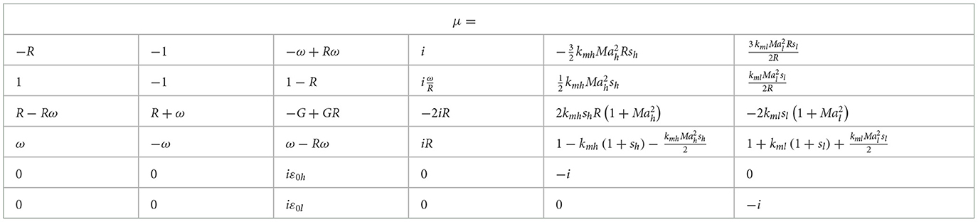
Table 4. Matrix M for the interfacial boundary value problem in the low Mach dynamics.

In the system M r = 0 (Equation 13), the vector r of the perturbation waves has the form:

$\begin{array}{l}r=({\stackrel{⌢}{\varphi }}_h{e}^{ix+z+\omega t},{\stackrel{⌢}{\varphi }}_l{e}^{ix-z+\omega t},\stackrel{⌢}{z}{e}^{ix},\\ {{\stackrel{⌢}{\psi }}_l{e}^{ix-\left(\omega /R\right)z+\omega t},{\stackrel{⌢}{e}}_h{e}^{ix+k_{h}z+\omega t},{\stackrel{⌢}{e}}_h{e}^{ix-k_{l}z+\omega t})}^{\text{T}}& (18.2)\end{array}$

In Table 4, the elements of the matrix μ depend on ω and the dimensionless quantities (R, G, (k_m, ε₀, Ma, s)_h(l)). In the matrix M = M(ω, R, G, (k_m, ε₀, Ma, s)_h(l)), the terms (k_m)_h(l) are given for completeness. They can be omitted, since the thermal transport is vanishing as (k_m)_h(l) → 0 with ${(k_m/M{a}^2)}_{h(l)}\to 0$, and the low Mach dynamics is weakly compressible ${(M{a}^2)}_{h(l)}<<1$.

In the dimensionless form, the fundamental solutions are r_i = r_i(ω_i, e_i). Each has the eigenvalue ω_i, the eigenvector e_i, and the associated amplitude vector ${\widehat{\text{e}}}_i$ of the perturbation waves:

$\begin{array}{ll}r=C_i{r}_i,r_i=r_i\left({\omega }_i,e_i\right),{\widehat{e}}_i={\left({\stackrel{⌢}{\varphi }}_h,{\stackrel{⌢}{\varphi }}_l,\stackrel{⌢}{z},{\stackrel{⌢}{\psi }}_l,{\stackrel{⌢}{e}}_h,{\stackrel{⌢}{e}}_l\right)}_i^{\text{T}}& (18.3)\end{array}$

Table 5 presents in the dimensionless form the matrixes (P, S), with M = (S − ωP), in the low Mach dynamics. In the matrix P , the fifth and six rows (columns) have null elements. Hence, det P = 0, the inverse matrix P^-1 is undefined. This suggests a degeneracy of the low Mach dynamics and a smaller number of fundamental solutions than the number 6 of the degrees of freedom (Equation 13.3) [15, 16, 29, 61].

Table 5

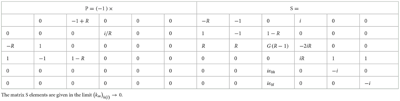
Table 5. Matrices (P,S), with M = (S − ωP), in the low Mach dynamics.

3.3 Fundamental solutions

In the low Mach dynamics, the fundamental solutions have the following attributes:

(1) The low Mach dynamics is degenerate. It has only four fundamental solutions r_1(2)(3)(4) for the six equations with the six degrees of freedom. Mathematically, the degeneracy is associated with the matrix P, for which the inverse matrix P^-1 is undefined. Physically, the degeneracy is due to the thermodynamic (rather than mechanical) nature of the internal energy perturbations (ē)_h(l); these perturbations are due to the seeds of the thermal heat flux with (ē)_h(l)(ε₀)_h(l) (see also the works [15, 16, 29, 61]).

(2) For the fundamental solutions r₁₍₂₎, the potential and vortical fields of the velocity are coupled with the interface perturbation and with the thermal heat flux. In case of the null thermal heat flux, the velocity fields are potential in both fluids. The fundamental solutions r₁₍₂₎ depend on the density ration, the acceleration strength, and the seeds of the thermal heat flux (R, G, (ε₀)_h(l)). These solutions are independent of the parameters (k_m, Ma, s)_h(l) in the low Mach dynamics (see also the work [16]).

(3) The fundamental solutions r₃₍₄₎ depend only on the density ratio R. These solutions are the same as the corresponding solutions for the conservative dynamics in ideal fluids in the absence of the thermal heat flux. They do not contribute to the dynamics (see also the works [15, 16, 29, 30]).

The fundamental solutions r₁₍₂₎ depend on the parameters (R, G, (ε₀)_h(l)). The solution r₁ can be stable or unstable. The solution r₂ is stable. We define the solution r_CDGM, where the subscript stands for the conservative dynamics (CD) under the gravity (G) in the low Mach (M) dynamics. For a real eigenvalue ω₁, the solution r_CDGM is the fundamental solution r₁, as r_CDGM = r₁, with the eigenvalue ω_CDGM = ω₁, the eigenvector e_CDGM = e₁, and the amplitude vector ${\widehat{\text{e}}}_{CDGM}={\widehat{\text{e}}}_1$. For an imaginary eigenvalue ω₁, the solution r_CDGM is given by the fundamental solutions r₁ and r₂ (with ${\text{r}}_1={\text{r}}_2^{*}$, ${\omega }_1={\omega }_2^{*}$ and ${\text{e}}_1={\text{e}}_2^{*}$), as ${\text{r}}_{CDGM}=({\text{r}}_1+{\text{r}}_1^{*})/2$; the asterisk marks the complex conjugate.

For the solution r_CDGM, the heavy fluid velocity is represented by the potential field, u_h = ∇Φ_h with ${\Phi }_h={(\bar{\Phi }+{\bar{\Phi }}_e)}_h$, whereas the light fluid velocity is given by the potential and vortical fields, u_l = ∇Φ_l + ∇ × Ψ_l with ${\Phi }_l={(\bar{\Phi }+{\bar{\Phi }}_e)}_l$ and Ψ_l = (0, Ψ_l, 0). In the solution r_CDGM, the growth rate ω_CDGM and the amplitude vector ${\widehat{\text{e}}}_{CDGM}={({\stackrel{⌢}{\varphi }}_h,{\stackrel{⌢}{\varphi }}_l,\stackrel{⌢}{z},{\stackrel{⌢}{\psi }}_l,{\stackrel{⌢}{e}}_h,{\stackrel{⌢}{e}}_l)}_{CDGM}^{\text{T}}$ are:

$\begin{array}{l}{\omega }_{CDGM}=\pm i\sqrt{R}\sqrt{1-G\frac{(R+1)}{R(R-1)}-2\frac{({\epsilon }_{0h}+{\epsilon }_{0l})}{{(R-1)}^2}},\\ {\widehat{\text{e}}}_{CDGD}={(*,*,1,*,*,*)}^{\text{T}}& (19.1)\end{array}$

The symbol * stands for functions on (R, G, (ε₀)_h(l)). These functions are explicitly given in Table 6.

Table 6

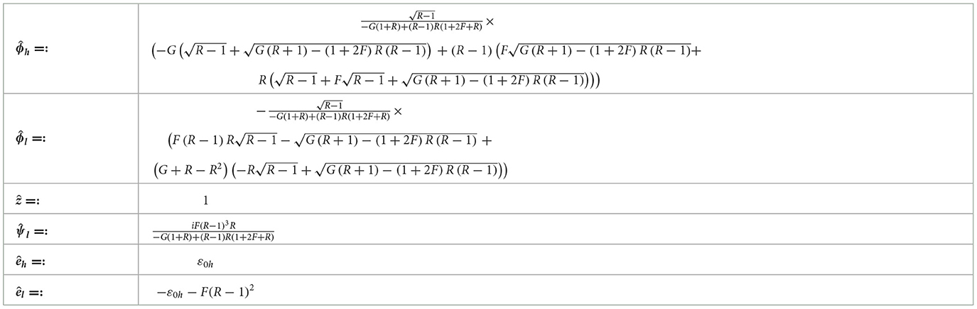
Table 6. Amplitude vector ${\widehat{\text{e}}}_{CDGM}={({\stackrel{⌢}{\varphi }}_h,{\stackrel{⌢}{\varphi }}_l,\stackrel{⌢}{z},{\stackrel{⌢}{\psi }}_l,{\stackrel{⌢}{e}}_h,{\stackrel{⌢}{e}}_l)}_{CDGM}^{\tau }$ for the solution r_CDGM.

We introduce the critical acceleration G_cr = R(R − 1)/(R + 1), the same as in the conservative dynamics in ideal fluids [15, 16]. We introduce the parameter $F=-({\epsilon }_{0h}+{\epsilon }_{0l})/{(R-1)}^2$ of the thermal heat flux [16]. The growth rate is transformed to:

$\begin{array}{ll}{\omega }_{CDGM}=\pm i\sqrt{R}\sqrt{(1+2F)-\frac{G}{G_{cr}}}& (19.2)\end{array}$

The dynamics r_CDGM is stable Re [ω_CDGM] ≤ 0 for the accelerations G < Ḡ_cr and is unstable Re [ω_CDGM] > 0 for G > Ḡ_cr. The ‘thermal' critical acceleration Ḡ_cr is Ḡ_cr = G_cr(1+2 F) [16].

The fundamental solution r₂ is stable in the stable regime, where the eigenvalue is imaginary, with ${\text{r}}_2={\text{r}}_1^{*}$, ${\omega }_2={\omega }_1^{*}$, ${\text{e}}_2={\text{e}}_1^{*}$, and with ${\text{r}}_{CDGM}=({\text{r}}_1+{\text{r}}_1^{*})/2$. The solution r₂ is stable, even when the growth rate ω_CDGM = ω₁ is real and the dynamics r_CDGM = r₁ is unstable. In this case, the integration constant C₂ = 0 must be zero, for the waves of the solution r₂ to satisfy the boundary conditions far away from the interface (Equation 9).

For the fundamental solution r₃, the eigenvalue ω₃ and the amplitude vector ${\widehat{\text{e}}}_3$ are:

$\begin{array}{ll}{\omega }_3=R,{\widehat{\text{e}}}_3={(0,i,0,1,0,0)}^{\text{T}}& (20.1)\end{array}$

While this solution is unstable, its perturbation fields for the velocity and the pressure are null for any integration constant. The solution r₃ does not contribute to the dynamics of thermally conducting fluids, similarly to the conservative dynamics in ideal fluids [15, 16, 29, 30]. We believe that the solution r₃ is due to the arbitrariness of choice of the inertial frame of reference.

For the fundamental solution r₄, the eigenvalue ω₄ and the amplitude vector ${\widehat{\text{e}}}_4$ are:

$\begin{array}{ll}{\omega }_3=-R,{\widehat{\text{e}}}_3={\left(\frac{2i}{R+1},-i\frac{R-1}{R+1},0,0,0,0\right)}^{\text{T}}& (20.2)\end{array}$

While this solution is stable, its integration constant must be zero, C₄ = 0, for the perturbation waves to satisfy the boundary conditions far away from the interface (Equation 9) (see also the works [15, 16, 29, 30]).

Figures 2–5 represent the perturbed fields of the velocity u, the velocity streamlines s, the pressure p, the vorticity ∇ × u, the internal energy ē, and the interface perturbation z^* in the stable and unstable low Mach dynamics r_CDGM, free from and under the destabilizing acceleration, and for vanishing and finite values of the parameter of the thermal heat flux.

Figure 2

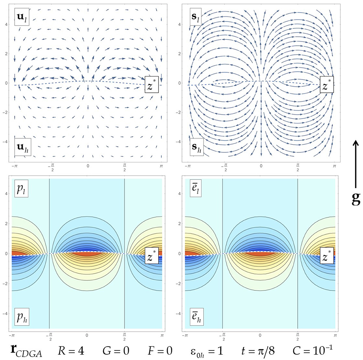
Figure 2. Flow fields for the inertial low Mach dynamics in thermally conducting fluids, when the thermal heat flux parameter is zero. Plots of real parts of perturbed fields of the interface, the velocity, the velocity streamlines, the pressure, and the internal energy, with red (blue) for positive (negative) in the contour plots. The perturbed vortical and vorticity fields are null.

Figure 3

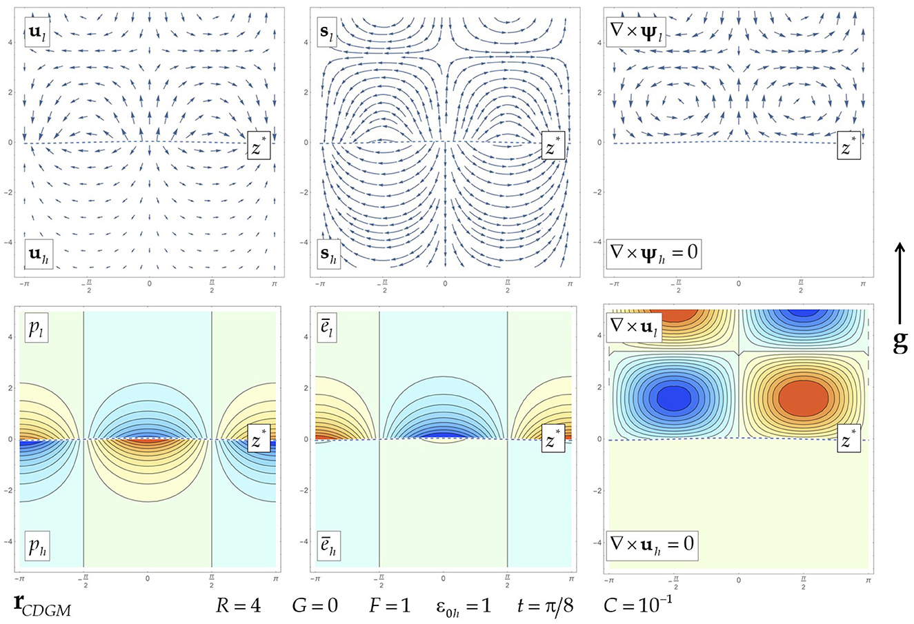
Figure 3. Flow fields for the inertial low Mach dynamics in thermally conducting fluids, when the thermal heat flux parameter is finite. Plots of real parts of perturbed fields of the interface, the velocity, the velocity streamlines, the pressure, the vorticity, and the internal energy, with red (blue) for positive (negative) in the contour plots.

Figure 4

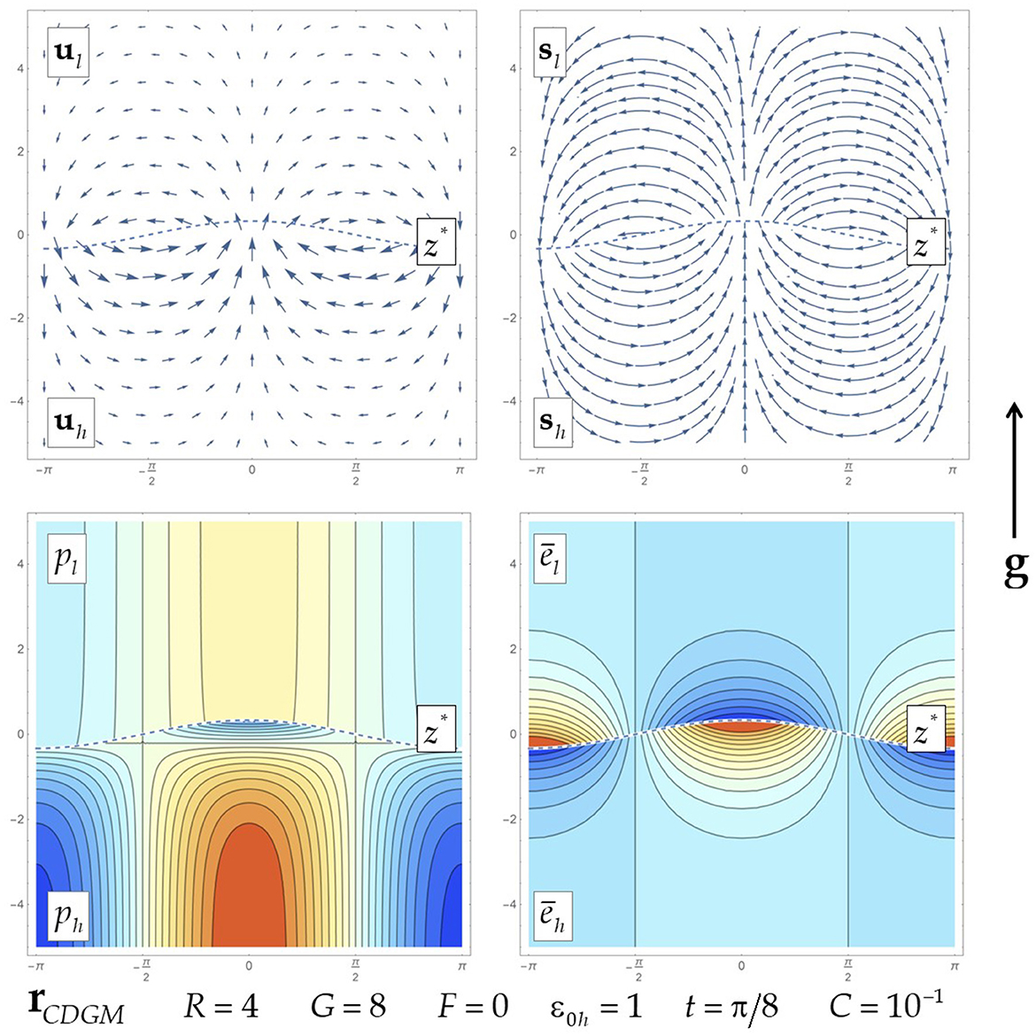
Figure 4. Flow fields for the unstable low Mach dynamics in thermally conducting fluids, under the destabilizing acceleration, when the thermal heat flux parameter is zero. Plots of real parts of perturbed fields of the interface, the velocity, the velocity streamlines, the pressure, and the internal energy, with red (blue) for positive (negative) in the contour plots. The perturbed vortical and vorticity fields are null.

Figure 5

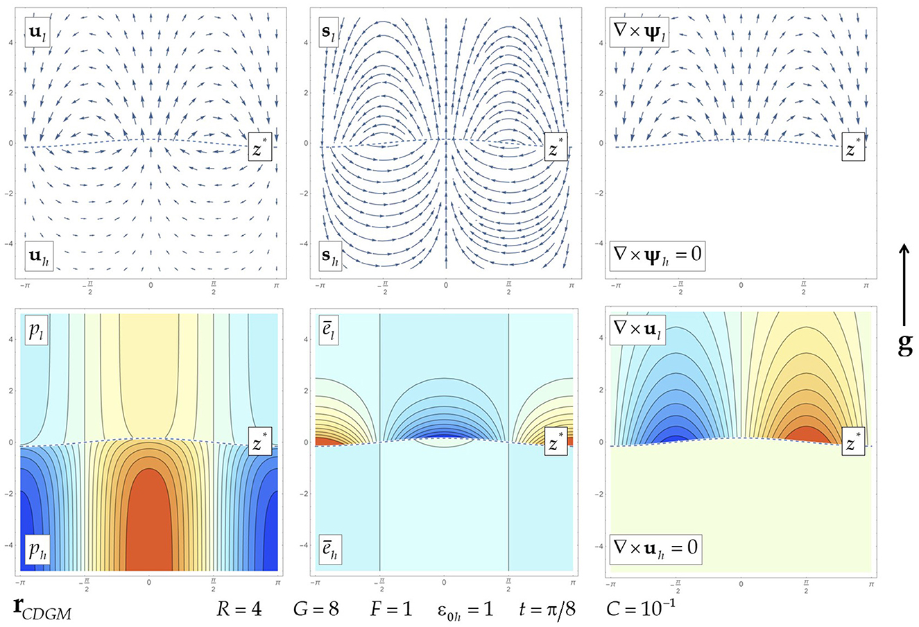
Figure 5. Flow fields for the unstable low Mach dynamics in thermally conducting fluids under the destabilizing acceleration, when the thermal heat flux parameter is finite. Plots of real parts of perturbed fields of the interface, the velocity, the velocity streamlines, the pressure, the vorticity, and the internal energy, with red (blue) for positive (negative) in the contour plots.

3.4 Thermal heat flux

We briefly outline a few effects of the thermal heat flux on the low Mach dynamics r_CDGM.

When the seeds of the thermal heat flux are null (ε_0h(l) = 0, F = 0), the vortical field is null, the energy perturbations are null, and the solution r_CDGM in thermally conducting fluids is:

$\begin{array}{l}{{\omega }_{CDGM}|}_{F=0}=\pm i\sqrt{R}\sqrt{1-\frac{G}{G_{cr}}},\\ {{\widehat{\text{e}}}_{CDGD}|}_{{\epsilon }_{0h(l)}=0,F=0}={(*,*,1,0,0,0)}^{\text{T}}& (20.1)\end{array}$

It is the same as the solution r_CDG for the conservative dynamics in ideal fluids [15]. For the null seeds of the thermal heat flux, the thermal conductivity effectively plays no role in the low Mach dynamicsr_CDGM (see Equations 14–17, 19 and Table 6).

The energy perturbations are identified through the leading order interfacial boundary condition for the energy (Equation 6.4). With seeds of the thermal heat flux (Q₀)_h(l) = (Je₀ε₀)_h(l), it is transformed to:

$\begin{array}{l}\left[{\epsilon }_0{e}_0+\frac{V^2}{2}+W_0\right]=0\\ \Rightarrow {{\epsilon }_{0l}|}_{\theta =0}={\left({\epsilon }_{0h}\frac{e_{0h}}{e_{0l}}-\frac{V_h^2}{2e_{0l}}\left({\left(\frac{{\rho }_h}{{\rho }_l}\right)}^2-1\right)+\frac{\left(W_{0h}-W_{0l}\right)}{e_{0l}}\right)|}_{\theta =0}& \left(20.2\right)\end{array}$

In the incompressible limit [W₀] = 0, by presuming that the heavy fluid is cold and is free from the thermal heat flux, ε_0h = 0, and that the light fluid is hot and has the thermal heat flux, ε_0l ≠ 0, the seed value is ε_0l < 0; hence, the thermal heat flux parameter F~ − (ε_0h + ε_0l) is F > 0. Here, we study the case F > 0. These situations may occur in the processes of combustion and plasma fusion [5, 6, 12–16, 45–54]. Our theory can be extended to the cases F < 0 that may occur in, e.g., chemically reacting fluids, as well as to the compressible case [W₀] ≠ 0 to be studied elsewhere.

Per the properties of the amplitude vector in Table 6, in the low Mach dynamics, the vortical field exists only in the presence of the thermal heat flux parameter ${\stackrel{⌢}{\psi }}_l~iF$. The vortical potential Ψ_l is shifted by π/2 relative to the fields of the velocity potentials Φ_h(l), the internal energy perturbations ē_h(l), the pressure p_h(l), and the interface perturbation z^* for any values (F > 0, R > 1, G ≥ 0).

3.5 Inertial dynamics

Consider the inertial low Mach dynamics, with null acceleration, G = 0, with r_CDGM → r_CDM:

$\begin{array}{l}{{\omega }_{CDGM}|}_{G=0}={\omega }_{CDM}=\pm i\sqrt{R}\sqrt{(1+2F)},\\ {{\widehat{\text{e}}}_{CDGD}|}_{G=0}={\widehat{\text{e}}}_{CDGD}|={(*,*,1,*,*,*)}^{\text{T}}& (21)\end{array}$

The dynamics r_CDM is stable for F > 0 (formally, for F > −1/2).

Figures 2, 3 illustrate the flow fields in the inertial low Mach dynamics in thermally conducting fluids for the vanishing and finite values of the thermal heat flux parameter, in consistency with Table 6. At F = 0 in both fluids, the velocity field is potential and the fields of the pressure and the energy perturbations are symmetric. For a finite value F, the energy perturbations become asymmetric in the heavy and the light fluids, and the velocity has the vortical field in the light fluid bulk.

Since the growth rate is purely imaginary, ${\omega }_{CDM}=\pm i\sqrt{R}\sqrt{(1+2F)}$, the wave vector of the vortical field K_ψl = ω_CDM/R is imaginary. This creates a stable vortical pattern, periodic in time and in space, in the bulk of the light fluid. The vortical structures can be realized when the boundary conditions away from the interface are somewhat noisy. Otherwise, the integration constant for the stable solution r_CDGM must be zero, leading to zero perturbation fields and constant interface velocity $\tilde{\text{V}}={\tilde{\text{V}}}_0$.

Consider the vortical field with the amplitude ${\stackrel{⌢}{\psi }}_l$ and wave vector K_ψl, and the energy field ${\stackrel{⌢}{e}}_l$ in the light fluid:

$\begin{array}{l}{\stackrel{⌢}{\psi }}_l=-i\frac{F{(R-1)}^{2}R}{R(R+1+2F)},K_{{\psi }_l}=i\sqrt{\frac{1+2F}{R}},\\ {\stackrel{⌢}{e}}_l=-{\epsilon }_{oh}-F{(R-1)}^2& (22.1)\end{array}$

The amplitude of the vortical field $\left|{\stackrel{⌢}{\psi }}_l\right|$ increases with the thermal heat flux F and the density ratio R. The wave vector of the vortical field |K_ψl| increases with F and decreases with R. The energy field $\left|{\stackrel{⌢}{e}}_l\right|$ increases with the thermal heat flux F and the density ratio R. For a small thermal heat flux parameter $F^{~}{0}^{+}$, for fluids with similar, $R^{~}{1}^{+}$, and different, R → ∞ , densities, these quantities are:

$\begin{array}{l}F\to 0^{+},R\to 1^{+}\Rightarrow {\stackrel{⌢}{\psi }}_l\approx -i\frac{F{\left(R-1\right)}^2}{2},\\ K_{{\psi }_l}\approx i\left(1+F+\frac{R-1}{2}\right),{\stackrel{⌢}{e}}_l\approx -{\epsilon }_{oh}& \left(22.2\right)\end{array}$

$\begin{array}{l}F\to 0^{+},R\to \infty \Rightarrow {\stackrel{⌢}{\psi }}_l\approx -iFR,\\ K_{{\psi }_l}\approx i(1+F)\sqrt{R},{\stackrel{⌢}{e}}_l\approx -{\epsilon }_{oh}-F{R}^2& (22.3)\end{array}$

For a large thermal heat flux parameter, F → ∞ , these quantities are:

$\begin{array}{l}F\to \infty ,R\to 1^{+}\Rightarrow {\stackrel{⌢}{\psi }}_l\approx -i\frac{{\left(R-1\right)}^2}{2},\\ K_{{\psi }_l}\approx i\sqrt{2}F\left(1+\frac{\left(R-1\right)}{2}\right),{\stackrel{⌢}{e}}_l\approx -{\epsilon }_{oh}-F{\left(R-1\right)}^2& \left(22.4\right)\end{array}$

$\begin{array}{l}F\to \infty ,R\to \infty \Rightarrow {\stackrel{⌢}{\psi }}_l\approx -i\frac{R^2}{2},\\ K_{{\psi }_l}\approx i\sqrt{F}\sqrt{R},{\stackrel{⌢}{e}}_l\approx -F{R}^2& \left(22.5\right)\end{array}$

In the inertial low Mach dynamics, the vortical field has no characteristic length scale, in contrast to the inertial Landau dynamics in Landau–Darrieus instability [20, 29].

Consider the interface velocity $\tilde{\text{V}}={\tilde{\text{V}}}_0+\tilde{\text{v}}$. It stably oscillates:

$\begin{array}{ll}\tilde{\text{v}}·{\text{n}}_0=-{(\text{u}·{\text{n}}_0+\stackrel{.}{\theta })|}_{\theta =0}\Rightarrow \tilde{\text{v}}·{\text{n}}_0~e^{i\left|{\omega }_{CDM}\right|t}& (23)\end{array}$

The expressions (Equations 21, 23) exhibit that in the inertial low Mach dynamics in thermally conducting fluids, the primary stabilization mechanism is the inertial mechanism. See the works [15] explored the inertial stabilization of the conservative dynamics of ideal fluids. This macroscopic mechanism is due to the conservation of mass, momentum, and energy; it is associated with the motion of the interface as a whole. The thermal mass flux—microscopic in nature—influences the frequency of the stable oscillations and, for the thermal heat flux parameter F ≠ 0, it creates the vortical field in the bulk (Equations 21–23) (Table 6).

We now represent the frequency ω_CDM (Equation 21) in the dimensional form as:

$\begin{array}{l}{\Omega }_{CDGM}=\pm ik{\bar{V}}_h\sqrt{\frac{{\rho }_{0h}}{{\rho }_{0l}}},\\ \frac{{\bar{V}}_h}{V_h}=\sqrt{1+2\left({\left(\frac{{\text{Q}}_0·\text{J}}{{\text{J}}^2{e}_0}\right)}_h+{\left(\frac{{\text{Q}}_0·\text{J}}{{\text{J}}^2{e}_0}\right)}_l\right)\frac{{\rho }_{0l}^2}{{\left({\rho }_{0h}-{\rho }_{0l}\right)}^2}}& \left(24\right)\end{array}$

Since the energy seeds ${({\epsilon }_0)}_{h(l)}={({\text{Q}}_0·\text{J}/{\text{J}}^2{e}_0)}_{h(l)}$ are identified by the leading order energy balance in the expressions (Equation 6.4), the thermal heat flux keeps intact the linear dependence of the frequency on the wave vector Ω_CDM ~ k. The thermal heat flux changes the magnitude of the frequency Ω_CDM. The change may be interpreted as an effective rescaling of the interface velocity ${\tilde{\text{V}}}_0$.

3.6 Accelerated dynamics

Examine the low Mach dynamics under the destabilizing acceleration.

Per the expressions (Equation 19), the dynamics r_CDGM is stable for small acceleration, G ∈ (0, Ḡ_cr), and it is unstable for the acceleration magnitudes exceeding a threshold G > Ḡ_cr. In the stable dynamics r_CDGM, the frequency of the oscillations is ${\omega }_{CDGM}=\pm i\sqrt{R}\sqrt{(1+2F)-G/G_{cr}}$, and the flow fields are qualitatively similar to those in the inertial low Mach dynamics.

Figures 4, 5 present the flow fields in the unstable accelerated low Mach dynamics, G > Ḡ_cr, in thermally conducting fluids, with the vanishing and finite values of the thermal heat flux parameter, in consistency with Table 6. At F = 0 in both fluids, the velocity field is potential and the fields of the energy perturbations are symmetric. For a finite F value, the energy perturbation fields become asymmetric in the heavy and the light fluids, and the velocity has the vortical field in the bulk of the light fluid. The vortical field is shifted relative to the fields of the pressure and energy by π/2 (see Table 6). For given values of the density ratio R and the thermal heat flux F, the strength of the vortical field ${\stackrel{⌢}{\psi }}_l$ overall decreases with an increase of the gravity G, with $|{\stackrel{⌢}{\psi }}_l{|}^{~}{G}^{-1}$ for G → ∞ . The strength of the energy perturbation field(s) ${\stackrel{⌢}{e}}_{h(l)}$ is independent of the acceleration, and it is the same as that in the inertial dynamics, in consistency with Figures 2, 3, and Table 6.

The expression (Equation 19) exhibits that in the low Mach dynamics in thermally conducting fluids in the presence of the thermal heat flux, the interface stability is defined primarily by the interplay of the two macroscopic mechanisms—the stabilizing inertial mechanism and the destabilizing acceleration. The inertia dominates the buoyancy, and the dynamics is stable for G < Ḡ_cr. The buoyancy dominates the inertia, and the dynamics is unstable for G > Ḡ_cr [16]. This is similar to the interface stability in the conservative dynamics in ideal fluids [15]. The thermal heat flux—along with creating the vortical field—provides additional stabilizations [16]. Particularly, it enlarges the value of the acceleration threshold to Ḡ_cr = G_cr(1 + 2F), with Ḡ_cr→G_cr for F → 0 ⁺ and with Ḡ_cr ≈ 2FG_cr for F → ∞.

Consider the interface velocity $\tilde{\text{V}}={\tilde{\text{V}}}_0+\tilde{\text{v}}$. It is time-dependent:

$\begin{array}{ll}\tilde{\text{v}}·{\text{n}}_0=-{(\text{u}·{\text{n}}_0+\stackrel{.}{\theta })|}_{\theta =0}\Rightarrow \tilde{\text{v}}·{\text{n}}_0~e^{+\left|{\omega }_{CDGM}\right|t}& (25)\end{array}$

The unstable low Mach dynamics in thermally conducting fluids superposes the growth of the interface velocity as whole and the growth of the interface perturbation. These growths are exponential in time in the linear regime and are expected to be a power law in time in the non-linear regime, similarly to the conservative dynamics in ideal fluids [15].

We now represent the frequency ω_CDM (Equation 19) in the dimensional form as:

$\begin{array}{l}g>{ḡ}_{cr}:{\Omega }_{CDGM}=k{\bar{V}}_h\left(\frac{{\rho }_h}{{\rho }_l}\right)\sqrt{\frac{g}{{ḡ}_{cr}}-1};\\ {ḡ}_{cr}=k{\bar{V}}_h^2\left(\frac{{\rho }_h}{{\rho }_l}\right)\left(\frac{{\rho }_h-{\rho }_l}{{\rho }_h+{\rho }_l}\right)& \left(26.1\right)\end{array}$

where the rescaled velocity magnitude ${\bar{V}}_h$ is provided by the expression (Equation 24). For given values$(k,{\bar{V}}_h)$ for fluids with different densities and with similar densities, the critical acceleration is:

$\begin{array}{l}\frac{{\rho }_h}{{\rho }_l}\to \infty :\frac{{ḡ}_{cr}}{k{\bar{V}}_h^2}\approx \left(\frac{{\rho }_h}{{\rho }_l}\right)\to \infty ;\\ \frac{{\rho }_h}{{\rho }_l}\to 1^{+}:\frac{{ḡ}_{cr}}{k{\bar{V}}_h^2}\approx \frac{{\rho }_h-{\rho }_l}{2{\rho }_h}\to 0^{+}& \left(26.2\right)\end{array}$

For given values of the acceleration g > ḡ_cr, the energy seeds ${({\epsilon }_0)}_{h(l)}={({\text{Q}}_0·\text{J}/{\text{J}}^2{e}_0)}_{h(l)}$, and the fluid densities ρ_h(l), we find the critical wave vector k_cr stabilizing the dynamics:

$\begin{array}{ll}{{\Omega }_{CDGM}|}_{k=k_{cr}}=0:k_{cr}=\frac{g}{{\bar{V}}_h^2}\left(\frac{{\rho }_l}{{\rho }_h}\right)\left(\frac{{\rho }_h+{\rho }_l}{{\rho }_h-{\rho }_l}\right)& \left(27.1\right)\end{array}$

We further find the maximum wave vector k_max at which the unstable dynamics has the largest growth:

$\begin{array}{l}{\frac{\partial {\Omega }_{CDGM}}{\partial k}|}_{k=k_{max}}=0,{\frac{{\partial }^2{\Omega }_{CDGM}}{\partial k^2}|}_{k=k_{max}}<0:\\ k_{max}=\frac{1}{2}\frac{g}{{\bar{V}}_h^2}\left(\frac{{\rho }_l}{{\rho }_h}\right)\left(\frac{{\rho }_h+{\rho }_l}{{\rho }_h-{\rho }_l}\right)& \left(27.2\right)\end{array}$

From the expressions (Equations 26, 27), we obtain for any density ratio and for any thermal heat flux:

$\begin{array}{l}\frac{k_{max}}{k_{cr}}=\frac{1}{2},\frac{k_{cr}}{k}=\frac{g}{{ḡ}_{cr}},\frac{k_{max}}{k}=\frac{1}{2}\frac{g}{{ḡ}_{cr}},\\ \frac{{\Omega }_{CDGM}}{{{\Omega }_{CDGM}|}_{k=k_{max}}}=2\sqrt{\frac{{ḡ}_{cr}(g-{ḡ}_{cr})}{g^2}}& (27.3)\end{array}$

Remarkably, in the low Mach dynamics in thermally conducting fluids, the ratio is 1/2 of the maximum and critical wave vectors; it is the same as that in the conservative dynamics in ideal fluids [15]. This is because the seeds of the energy perturbations are defined by the leading order balance for the thermal heat flux (Equation 6.4). It keeps intact the dependences of the critical k_cr and maximum k_max wave vectors and their ratio k_cr/k_max on the acceleration g and the velocity V_h. At the same time, through the velocity rescaling, $V_h\to {\bar{V}}_h$ the thermal heat flux changes the values of the k_cr and k_max magnitudes. The critical wavelength λ_cr = 2π/k_cr and the maximum wavelength λ_max = 2π/k_max increase with the thermal heat flux.

Consider the effect of the density ratio on the dispersion curve and the maximum growth rate for given values of the thermal heat flux and the acceleration. For fluids with different densities in Equations 27.1–27.3, the critical and maximum wave vector and the growth rate are:

$\begin{array}{l}\frac{{\rho }_h}{{\rho }_l}\to \infty :k_{cr}\approx \frac{g}{{\bar{V}}_h^2}\frac{{\rho }_l}{{\rho }_h},k_{max}\approx \frac{g}{2{\bar{V}}_h^2}\frac{{\rho }_l}{{\rho }_h},\\ {{\Omega }_{CDGM}|}_{k=k_{max}}\approx \frac{g}{2{\bar{V}}_h}\sqrt{\frac{{\rho }_l}{{\rho }_h}}& (27.4)\end{array}$

For fluids with similar densities in Equations 27.1–27.3, these quantities are:

$\begin{array}{l}\frac{{\rho }_h}{{\rho }_l}\to 1^{+}:k_{cr}\approx \frac{2g}{{\bar{V}}_h^2}\frac{{\rho }_h}{{\rho }_h-{\rho }_l},k_{max}\approx \frac{g}{{\bar{V}}_h^2}\frac{{\rho }_h}{{\rho }_h-{\rho }_l},\\ {{\Omega }_{CDGM}|}_{k=k_{max}}\approx \frac{g}{{\bar{V}}_h}\frac{{\rho }_h}{{\rho }_h-{\rho }_l}& (27.5)\end{array}$

Hence, the dispersion curve is located at small wave vectors and small growth rates for fluids with different densities (Equation 27.4), and at large wave vectors and large growth rates for fluids with similar densities (Equation 27.5). This is consistent with quasi-homogeneity of the dynamics at small density ratios [15, 16].

4 Outcomes

Our theory investigates in detail the low Mach dynamics in thermally conducting fluids and finds the attributes not earlier discussed. This includes, e.g., the new fluid instability, the interplay of the destabilizing acceleration with the macroscopic inertial stabilization and the microscopic thermodynamics, and the link of the structure of the flow fields to the thermal heat flux. We compare our results with other theories and models, connect to existing experiments, outline the extensive theoretical benchmarks for experiments and simulations, and chart perspectives for future studies.

4.1 Comparison with models

The interface dynamics with interfacial fluxes of mass and heat is a long-standing problem in science, mathematics, and engineering [6, 11–14, 20, 47, 48]. Its traditional applications include the processes of premixed combustion (in the context of flame stability) and inertial confinement fusion (in the context of stability of laser ablated plasma) [2–14, 16, 20, 47–54].

4.1.1 Interface stability in fluids

Figure 6 presents the dependence of the growth rates on the acceleration magnitude for the low Mach dynamics in thermally conducting fluids with and without the thermal heat flux (Equation 24, 26) and for the classical Landau–Darrieus and Rayleigh–Taylor instabilities in ideal fluids. In Landau–Darrieus instability under gravity (LDG) and in Rayleigh–Taylor instability (RT), the growth rates are [14, 20, 21]:

$\begin{array}{l}{\Omega }_{LDG}=-\frac{k{V}_h{\rho }_h}{{\rho }_h+{\rho }_l}+\sqrt{gk\frac{{\rho }_h-{\rho }_l}{{\rho }_h+{\rho }_l}+{(k{V}_h)}^2\frac{{\rho }_h}{{\rho }_l}\frac{({\rho }_h^2+{\rho }_h{\rho }_l-{\rho }_l^2)}{{({\rho }_h+{\rho }_l)}^2}},\\ {\Omega }_{RT}=\sqrt{gk\frac{{\rho }_h-{\rho }_l}{{\rho }_h+{\rho }_l}}& (28)\end{array}$

Figure 6

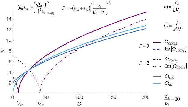
Figure 6. Dependence of the growth rate on the destabilizing acceleration of the low Mach dynamics and the classical Landau–Darrieus and Rayleigh–Taylor dynamics at some values of the density ratio and the thermal heat flux parameter.

For a given density ratio ρ_h/ρ_l and strong accelerations, g > > ḡ_cr, the unstable low Mach dynamics Ω_CDGM grows faster compared to Ω_LDG, and Ω_RT, achieving the largest growth for the zero heat flux.

The low Mach dynamics conserves mass, momentum, and energy in the bulk and, at the interface, and obeys the boundary conditions for the thermal heat flux at the interface. It is stabilized primarily by the inertial mechanism. In Landau–Darrieus instability, the Landau's dynamics conserves mass and momentum in the bulk and, at the interface, and is incompatible with the energy conservation at the interface. It postulates the constancy of the interface velocity and thus preempts the inertial stabilization mechanism to occur. In Rayleigh–Taylor dynamics, the inertial mechanism is absent due to the zero mass flux across the interface (see Equations 19, 21, 24, 26, Figure 6, and the works [3, 6, 11–14, 20, 21, 47, 48]).

In the low Mach dynamics, the velocity fields have potential and vortical components under the thermal heat flux and have only potential components at the zero thermal heat flux. In Landau–Darrieus dynamics, the velocity fields have potential and vortical components, whereas in Rayleigh–Taylor dynamics the velocity fields have only the potential component. In the low Mach dynamics, the velocity vortical field in the bulk is induced by the thermal heat flux, and the velocity is shear-free at the interface. In Landau–Darrieus dynamics, the velocity is shear-free at the interface, whereas Rayleigh–Taylor dynamics has the velocity shear at the interface. In the inertial frame of reference, the interface velocity is variable in the low Mach dynamics in both stable and unstable regimes, and it is constant in Landau–Darrieus dynamics and is zero in Rayleigh–Taylor dynamics. One can distinct between the low Mach dynamics and Landau–Darrieus/Rayleigh–Taylor dynamics by diagnosing the growth of the interface perturbations, the structure of flow fields in the bulk, and the interface velocity (see Equations 19, 24, 26, 28, Table 6 and Figure 6, and the works [3, 6, 11–14, 16, 20, 21, 28–30, 47, 48]).

4.1.2 Interface stability in plasmas

To directly compare our theoretical results with experiments in inertial confinement fusion, a scrupulous analysis of raw data is required. Since the data are a challenge to access, we compare the growth rates and dispersion relations in the low Mach dynamics and in the models of ablative Rayleigh–Taylor/Richtmyer–Meshkov instability in plasmas.

The pioneering models [49, 62] of ablative Rayleigh–Taylor instability suggest that in a single fluid, the growth rate is Ω_{B, AK} (subscript is for Bodner, Anisimov, Kull). For strong accelerations, this growth rate Ω_{B, AK} is in conformity with our results in Equations 24, 26:

$\begin{array}{l}{\Omega }_{B,AK}=-k{V}_a+\sqrt{gk},{{\Omega }_{B,AK}|}_{(g/k{V}_a^2)\to \infty }\to \sqrt{gk},\\ {{\Omega }_{CDGM}|}_{(g/k{V}_a^2)\to \infty }\to \sqrt{gk},\\ V_a={\bar{V}}_h& (29.1)\end{array}$

Here, the ablation velocity is V_a, and we set $V_a={\bar{V}}_h$. The pioneering works [50, 62] advise that ablative Richtmyer–Meshkov instability has a purely imaginary growth rate Ω_N (subscript is for Nishihara) for any density ratio. This is consistent with our results for the inertial dynamics in Equations 21, 24, 26:

$\begin{array}{ll}Re{\left[{\Omega }_N\right]=0,{\Omega }_{CDGM}|}_{(g/k{V}_a^2)=0}=\pm ik{V}_a\sqrt{\frac{{\rho }_h}{{\rho }_l}},V_a={\bar{V}}_h& (29.2)\end{array}$

The model [51] suggests the other growth rate in ablative Rayleigh–Taylor instability; the same expression is given in the model [52]; its growth rate is Ω_{SPI, B} (subscript is for Sanz, Piriz, Ibanez, Betti). The model [53] proposes for ablative Rayleigh–Taylor/Richtmyer–Meshkov instability the growth rate Ω_{G, AV} (subscript is for Goncharov, Aglitsky, Velikovich). They are:

$\begin{array}{l}{\Omega }_{SPI,B}=-k{V}_a\frac{2{\rho }_h}{{\rho }_h+{\rho }_l}+\sqrt{gk\frac{{\rho }_h-{\rho }_l}{{\rho }_h+{\rho }_l}-{\left(k{V}_a\right)}^2\frac{{\rho }_h}{{\rho }_l}{\left(\frac{{\rho }_h-{\rho }_l}{{\rho }_h+{\rho }_l}\right)}^2},\\ {\Omega }_{G,AV}=-2k{V}_a+\sqrt{gk-{\left(k{V}_a\right)}^2\frac{{\rho }_h}{{\rho }_l}}& \left(30.1\right)\end{array}$

For given values (k, V_a) in the models [51–53], the critical accelerations stabilizing the dynamics are:

$\begin{array}{ll}{g_{cr}|}_{PSI,B}=k{V}_a^2\frac{{\rho }_h}{{\rho }_l}\left(\frac{{\rho }_h+{\rho }_l}{{\rho }_h-{\rho }_l}\right),{g_{cr}|}_{G,AV}=k{V}_a^2\left(4+\frac{{\rho }_h}{{\rho }_l}\right)& \left(30.2\right)\end{array}$

In plasma fusion, the models [5, 46] are usually applied in a single fluid limit. For (ρ_h/ρ_l) → ∞ , the growth rates Ω_{SPI, B} Ω_{G, AV} are consistent with Ω_{B, AK} (at $g/k{V}_a^2>>1$) and Ω_N (at $g/k{V}_a^2<<1$) (Equation 29) [49, 50, 62, 63]. In the models [51–53] in Equation 30.1, for fluids with very different densities, the critical acceleration, the critical and maximum wave vectors, the maximum growth rate, and the frequency of the inertial dynamics are:

$\begin{array}{l}\frac{{\rho }_h}{{\rho }_l}\to \infty :{\frac{g_{cr}}{k{V}_a^2}|}_{CDGM(PSI,B)(G,AV)}\approx \frac{{\rho }_h}{{\rho }_l},{k_{cr}|}_{SPI,B(G,AV)}\approx \frac{g}{V_a^2}\frac{{\rho }_l}{{\rho }_h},\\ {k_{max}|}_{SPI,B(G,AV)}\approx \frac{k_{cr}}{2},\\ {{\Omega }_{SPI,B(G,AV)}|}_{k=k_{max}}\approx \frac{g}{2V_a}\sqrt{\frac{{\rho }_l}{{\rho }_h}},\\ {{\Omega }_{SPI,B(G,AV)}|}_{(g/k{V}_a^2)=0}\approx \pm ik{V}_a\sqrt{\frac{{\rho }_h}{{\rho }_l}}& (30.3)\end{array}$

This is consistent with our theory in the low Mach dynamics, upon the rescaling $V_a={\bar{V}}_h$, (Equations 24, 26, 27).

For purposes of completeness, we consider the models [51–53] for fluids with very similar densities $({\rho }_h/{\rho }_l)\to 1^{+}$. Then, the critical acceleration, the maximum and critical wave vectors, the maximum growth rate, and the frequency of the inertial dynamics are in the models [51, 52]:

$\begin{array}{l}\frac{{\rho }_h}{{\rho }_l}\to 1^{+}:{\frac{g_{cr}}{k{V}_a^2}|}_{PSI,B}\approx \frac{2{\rho }_h}{{\rho }_h-{\rho }_l},{k_{cr}|}_{SPI,B}\approx \frac{g}{2V_a^2}\frac{{\rho }_h-{\rho }_l}{{\rho }_h},\\ {k_{max}|}_{SPI,B}\approx \frac{g}{8V_a^2}\frac{{\rho }_h-{\rho }_l}{{\rho }_h},\\ {{\Omega }_{SPI,B}|}_{k=k_{max}}\approx \frac{g}{8V_a}\frac{{\rho }_h-{\rho }_l}{{\rho }_h},\\ {{\Omega }_{SPI,B}|}_{(g/k{V}_a^2)=0}\approx -k{V}_a\left(1\pm \frac{i}{2}\frac{{\rho }_h-{\rho }_l}{{\rho }_h}\right)& (30.4)\end{array}$

and they are in the model [53]:

$\begin{array}{l}\frac{{\rho }_h}{{\rho }_l}\to 1^{+}:{\frac{g_{cr}}{k{V}_a^2}|}_{G,AV}\approx 5,{k_{cr}|}_{G,AV}\approx \frac{g}{5V_a^2},\\ {k_{max}|}_{G,AV}\approx \frac{g}{2\sqrt{5}{V}_a^2}\left(\sqrt{5}-2\right),\\ {{\Omega }_{G,AV}|}_{k=k_{max}}\approx \frac{g}{10V_a}\left(5-2\sqrt{5}\right)\left(\sqrt{9+4\sqrt{5}}-2\right),\\ {{\Omega }_{G,AV}|}_{\left(g/k{V}_a^2\right)=0}\approx -k{V}_a\left(2\pm i\right)& \left(30.5\right)\end{array}$

These expressions depart from our theory of the low Mach dynamics (Equations 24, 26) and the works [15, 16].

Figure 7 presents the dependence of the critical acceleration $g_{cr}/k{V}_a^2$, scaled with $V_a={\bar{V}}_h$, on the density ratio ρ_h/ρ_l in the low Mach dynamics (Equations 24, 26) and in the models [51–53]. As expected (Equation 30), the models [51–53] are consistent with (depart from) our theory (Equations 26, 27) for fluids with very different (similar) densities.

Figure 7

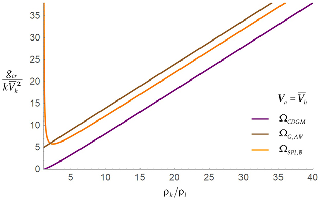
Figure 7. Dependence of the critical acceleration on the density ratio in the low Mach dynamics and the models of ablative Rayleigh–Taylor instabilities. The models are consistent with (depart from) the low Mach dynamics for fluids with very different (similar) densities.

Figure 8 presents the dependence of the growth rate Ω on the wave vector k in the low Mach dynamics (Equations 26, 27) and in the models [51–53]. The values are scaled with _{ΩCDGM|k = kmax}, _kcr|CDGM, and $V_a={\bar{V}}_h$ in the low Mach dynamics (Equations 26, 27). The dispersion curve in the models [51–53] is similar to that in our rigorous theory for very large density ratios (e.g., ${\rho }_h/{\rho }_l=4\times {10}^4$). For reasonably large density ratios (e.g., ρ_h/ρ_l = 40), the models [51–53] depart from our theory (Equations 26, 27) [16].

Figure 8

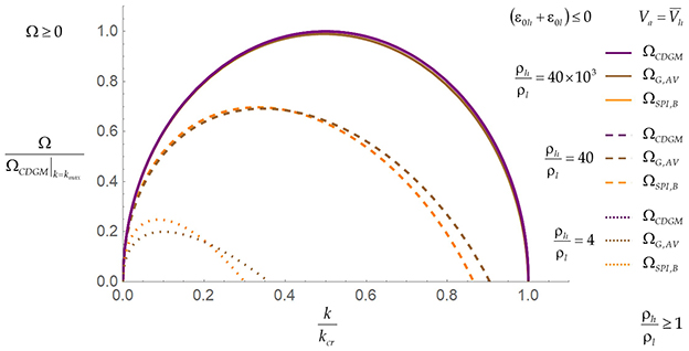
Figure 8. Dependence of the growth rate on the wave vector in the low Mach dynamics and the models of ablative Rayleigh–Taylor instabilities in the unstable regime. The dispersion curves in the models of ablative Rayleigh–Taylor instabilities coincide with that in the low Mach dynamics for very large density ratios. For large finite density ratios, the models of ablative Rayleigh–Taylor instabilities depart from the low Mach dynamics.

It is reported that the models [51–53] tend to agree with experiments at very large density ratios. By reproducing the results of the prior models for fluids with very different densities, our theory effectively agrees with the experimental data in fusion plasmas to the same (and, possibly, greater) extent [5, 46]. Our results illustrate the need for data availability and the importance of specific technical details, including the density ratio, the thermal heat flux, and the acceleration in the experiments (see Equations 24, 26 and Figure 6) [16, 46].

Our theory accurately finds the perturbation waves in the bulk, precisely formulates the boundary conditions for the thermal heat flux, and rigorously solves the boundary value problem at the interface. It finds the characteristics of the low Mach dynamics—as well as the advection and the diffusion dynamics—in a broad range of conditions, with (ρ_h/ρ_l) ∈ (1, ∞) and (K_m/k)_h(l) ∈ [0, ∞), well beyond the scope of the models [51–53]. This opens venues, unexplored before, for modeling interface dynamics in fusion plasmas. In particular, the growth of the unstable interface velocity additionally to the growth of the interface perturbations can explain a quick extinction of the hot spot in the inertial confinement fusion, which is observed in experiments [5, 46].

4.2 Comparison with observations

4.2.1 Prospect of Landau

Dynamics of an interface, having fluxes of heat and mass across it, is a long-standing challenge in mathematics, science, and engineering [6, 11–14, 20, 47, 48]. The classical theory of Landau [20] predicted that the interface with mass flux is unconditionally unstable, leading to Landau–Darrieus instability [14, 20]. For incompressible ideal fluids, the instability was a challenge to directly observe in the experiments [12–14]. The consensus addressing this paradox suggested the following: at small length scales, the interface dynamics is stabilized by microscopic thermodynamic mechanisms (e.g., viscosity, thermal conductivity, and surface tension). Large scale processes are difficult to realize in controlled laboratory environments [6, 12–14, 47].

Our theory resolves the paradox [20]. It finds [15, 16] that in both ideal and thermally conducting fluids, the interface is stabilized primarily by the macroscopic inertial mechanism and is destabilized by the acceleration. The microscopic thermodynamics and the thermal heat flux provide extra stabilizations and create vortical fields in the bulk. The unstable Landau's solution—by postulating constancy of the interface velocity—is a perfect mathematical match preempting the inertial mechanism to occur. Mathematical and physical properties of the multiphase dynamics found by our theory enable an unambiguous differentiation between the low Mach, Landau–Darrieus dynamics, and Rayleigh–Taylor dynamics in experiments and simulations, to be done in the future [3, 6, 14–16, 20, 21, 25–30].

4.2.2 Geophysics and astrophysics

Our theory finds that in the inertial low Mach dynamics, the interface is stable at global scales. This is consistent with and qualitatively explains the observations in geophysical multiphase flows [16, 35, 69]. The latter include the confluence of Green and Colorado Rivers and the stable border between the Pacific and Atlantic oceans. In these cases, distinct waters meet and do not mix, and the interface between the waters is globally stable [35, 69]. Our theory further finds that in the unstable accelerated low Mach dynamics, the interface velocity increases with time and the interface is free from the shear-driven vortical structures. These characteristics can aid better understanding of dynamics and morphology of filamentary structures in supernova remnants [3, 4].

4.2.3 Experiments in plasmas

The scaled laboratory experiments in high energy density plasmas examine the interfacial mixing of matters in supernova relevant conditions [46, 54]. The experiments [54] investigated the effect of the thermal heat flux on the interface stability and observed qualitative differences between the dynamics with high and low thermal heat flux values. Our theory is consistent with these observations [16, 54].

We find that in the experiments [54], the low flux case corresponds to the classical Rayleigh–Taylor instability, whereas the high flux case is related to the accelerated interfacial dynamics with mass and heat fluxes. Per our theory, these dynamics have distinct qualitative and quantitative properties (Equations 24, 26, 28, Figure 6); these distinctions explain the experimental observations [16].

Particularly, (i) in the low flux case in Rayleigh–Taylor dynamics, the interface perturbations grow quicker than in the unstable interfacial dynamics in the high flux case because the accelerations in the experiments are relatively low. (ii) In the unstable interfacial dynamics in the high flux case, the interfacial structure propagates quicker than in Rayleigh–Taylor dynamics in the low flux case because the inertial mechanism enlarges the velocity of the interface as a whole. (iii) The interface dynamics with fluxes of mass and heat is free from the interfacial shear and from shear-driven vortical structures at the interface. In Rayleigh–Taylor dynamics with the null mass flux, the shear and the vortical structures are present at the interface. This explains the distinctions in the interface morphology observed in the experiments in the high flux case and the low flux case (see Equations 24, 26, 28, Figure 6) [16, 54, 64].

4.2.4 Experiments in complex fluids

In our theory, the mass flux and the heat flux are separate physical quantities allowing one to independently analyze their contributions to the dynamics. This consideration is applicable in a broad range of conditions, including the microscopically thin interfaces with macroscopically observable mass and heat fluxes found in the experiments and molecular dynamics simulations [7–10, 18, 39, 44]. Our theory highlights the need in experimental systems that can autonomously control the flux of mass and the flux heat, or—in other words—the flux of mass and the flux of energy (Equations 24, 26, 28) [15, 16]. While such conditions may be a challenge to reach in regular fluids or plasmas, they may be achievable in complex matters involving chemical processes and transports of species and charges.

The experiments [39] investigated the chemical process of liquid–liquid extraction with the metastable precipitation and the transports of ions. This process is accompanied by the formation of interfaces separating the phases of matter (i.e., the liquids). The chemistry of the process controls the flux of mass and the flux of energy at and across the interfaces. The experimental system exhibits rich dynamics. This includes the formation of quasi-convective vortical structures associated with the energy imbalance at the interface, and quasi Rayleigh–Taylor fingering structures occurring when the fluxes of mass and energy across the interface are reduced [39]. The observations are in qualitative agreement with our theoretical results. In addition, the experiments and theory are consistent with the molecular dynamics simulations revealing complexity of energy transport in energetic materials and in reactive systems [18, 39].

4.2.5 Experiments on contained turbulence

Our theory identifies opportunities, not discussed before, for realizing turbulence in a laboratory.

It is traditionally believed that turbulence develops from a laminar flow via a tangential discontinuity mechanism, or a velocity shear. In this mechanism, the velocity shear at the discontinuity—the thin interface with zero mass flux across it—makes the interface unstable due to the Kelvin–Helmholtz instability and creates vortical structures at the interface [14]. The vortical structures are then presumed to propagate to the bulk, causing turbulence to develop [14, 65, 66].

Our theory suggests another mechanism of generating vortical fields and vortical structures in the bulk. We find that for an interface with fluxes of mass and energy, the velocity field is free from the interfacial shear. The vortical field in the bulk is created by the energy flux across the interface. For the stable interface, the vortical field is represented by periodic vortical structures. They may cause turbulence to develop (see Equations 24, 26, 28 and the works [15, 16, 29]).

The experiments [55] examined how to create turbulence in a contained geometry, free from using extended tunnels and applying a velocity shear as it is done in turbulent boundary layers or a jet turbulence [65, 66]. The experiments employ a ring of jets to blow loops—vortex rings—into a tank of water until an isolated ball of turbulence forms and lasts, thus observing a contained turbulence in the tank. These observations are in a qualitative consistency with our theoretical results (Equations 24, 26, 28) and with the works [15, 16, 29]. Particularly, the turbulence ball is isolated; it is effectively separated from the ambient by a self-formed interface; the mass and energy are transported through the interface; hence, turbulence can develop. By using our theory [15, 16, 29] and the experiments [55], one can directly examine Kolmogorov turbulence—a process driven by an external energy source causing strong stochastic fluctuations [14, 37, 38, 67, 68].

4.3 Benchmarks and diagnostics

By finding benchmarks of interface dynamics not earlier diagnosed, our theory opens opportunities for experiments and simulations (see Equations 12–27, Tables 1–6, Figures 2–8) [16].

For validating the low Mach dynamics in experiments and simulations, it is required, in addition to the velocity vector field, to precisely measure the scalar fields of the inertial energy, the density, and the pressure. These fields are correlated (Equations 14–17). In the heavy (light) fluid, they have the initial perturbation length scale ${\tilde{k}}_h^{-1}({\tilde{k}}_l^{-1})$ and are modulated with waves with the length scale ${\tilde{k}}_h^{-1}({\tilde{k}}_l^{-1})$. In the low Mach dynamics, the length scale ${\tilde{k}}_h^{-1}({\tilde{k}}_l^{-1})$ is independent of the thermal conductivity and is greater than the length scale of the initial perturbation $k{\tilde{k}}_{h\left(l\right)}^{-1}<<1$ (see Equations 14–17, Tables 1–3, Figures 2–5) [16].

Our theory directly links macroscopic attributes of the low Mach dynamics (the vortical structures in the bulk and the interface stability) to the microscopic thermodynamic properties (the thermal heat flux and the thermal conductivity). To qualitatively detect the presence of the thermal heat flux at the interface, one has to measure the velocity vortical and vorticity fields in the bulk; these fields are produced by the energy excess (i.e., the thermal heat flux) at the interface. To quantify the thermal heat flux at the interface, one has to accurately balance the values of the specific enthalpy W₀ and the specific kinetic energy $({\text{J}}^2/2{\rho }_0^2)$, where the physical enthalpy is $W_0={\bar{W}}_0+C_P\Theta$ , the enthalpy of formation is ${\bar{W}}_0$, the specific heat at constant pressure is C_P, and the temperature is Θ (see Equations 19–27, Tables 4–6, Figures 2–6) [16].

In the low Mach dynamics, the interface stability is defined primarily by the macroscopic inertial mechanism balancing the destabilizing acceleration, and the thermal heat flux creates vortical fields in the bulk. The instability of the low Mach dynamics in thermally conducting fluids differs qualitatively and quantitatively from the instability of the conservative dynamics in ideal fluids. The low Mach dynamics has the potential and vortical velocity fields, whereas the conservative dynamics has only the potential velocity fields. Remarkably, in the unstable low Mach dynamics for the maximum and critical wave vectors, the ratio is the same as that in the conservative dynamics; the growth rates of these dynamics can be linked with one another upon appropriate velocity scaling (see Equations 25–27, Table 6, Figure 6) [16].

Our rigorous theory inspires the experiments and simulations to further advance diagnostics and the data' accuracy, precision, and statistics, for better understanding multiphase dynamics. In realistic fluids, in addition to the interface growth and growth rate, experimental diagnostics have to include the structure of the macroscopic fields in the bulk, the properties of microscopic transports at the interface, and the unsteadiness of the interface velocity. In high energy density plasmas, the experiments have to employ the capabilities of high power laser facilities in pulse shaping and in target fabrication for precise controlling the thermal heat flux and the thermal transport. In materials, for better understanding the interplay of mass and energy transports at the interface, one can employ the highly accurate experiments in complex fluids, and the Eulerian and Lagrangian methods of numerical modeling (see Equations 19–27, Table 6, Figures 2–8) [5–10, 18, 19, 32–34, 39, 42–46, 54–59, 64–66].

The advancements in experimental and numerical approaches enable one to quantify with high fidelity and ample statistics the microscopic transport at the interface and the macroscopic fields in the bulk. In synergy with our theory, they can provide new insights in far from equilibrium dynamics of interfaces and interfacial mixing in nature, technology, and industry (see the works [1, 2]).

5 Summary

We examine analytically the classical problem of the interface dynamics with the interfacial fluxes of mass and heat in thermally conducting inviscid fluids. The low Mach regime is thoroughly investigated, in which the flow fields are subsonic (including the uniform fields and the perturbation waves), the thermal conductivity length scale is large compared to that of the initial perturbation, and the weak compressibility dominates over the thermal transport (see Equations 1–4) [16].

We employ the rigorous theoretical framework to solve this long-standing problem [15, 16]. By using the generalized functions, the boundary conditions at the interface are self-consistently derived from the governing equations in the bulk, including the conditions for the fluxes of mass, momentum, and energy and for the thermal heat flux. The thermal heat flux at the interface and the seeds of perturbations of the internal energy are accurately evaluated. We precisely identify the degrees of freedom of the dynamics, including the four mechanical perturbation waves and the two energetic waves seeded by the internal energy perturbations. We solve the boundary value problem in a broad range of parameters and find the growth of the interface and the structure of the flow fields in the bulk, thus linking the processes at micro and macro scales (see Equations 5–17, Tables 1–5).

The low Mach dynamics possess the following characteristics. The interface is stabilized primarily by the macroscopic inertial mechanism that balances the destabilizing acceleration. The microscopic thermodynamics and the thermal heat flux provide additional stabilizations. The interface is unstable, when the dynamics is accelerated, and the acceleration magnitude exceeds a threshold. The interface is globally stable, if the dynamics is inertial. The thermal heat flux at the interface forms the vortical and vorticity velocity fields in the bulk. The vortical field is energetic—rather than dynamic—in nature. For the zero thermal heat flux, the internal energy perturbations vanish, and the velocity has only potential fields in the bulk. The velocity field is free from the shear at the interface (see Equations 18–27, Table 6, Figures 2–5).

In the inertial frame of reference, the low Mach dynamics is a superposition of the two motions—the dynamics of the interface as a whole and the dynamics of the interface perturbations. The velocity of the interface is variable. In the stable regime, it oscillates along with oscillations of the interface perturbations. In the unstable regime, its magnitude increases in time, along with the amplitude growth of perturbations of the interface and the flow fields. The low Mach dynamics is degenerate; it has the smaller number of the fundamental solutions than the number of the degrees of freedom. The degeneracy is due to the thermodynamic nature of the internal energy perturbations. For the zero thermal heat flux parameter, the low Mach dynamics in thermally conducting fluids coincides with the conservative dynamics in ideal fluids (see Equations 19–27, Tables 5, 6, Figures 2–6) [16].

Qualitative and quantitative properties reveal that the low Mach dynamics differ substantially from the dynamics of the Landau–Darrieus and Rayleigh–Taylor instabilities. One can clearly distinguish in experiments and simulations between the low Mach, Landau–Darrieus, and Rayleigh–Taylor dynamics, to be done in the future. Our theory accurately reproduces in certain limiting cases the results of the models of ablative Rayleigh–Taylor instability. Our approach is applicable in a broad range of the acceleration magnitudes, the thermal heat flux values, and the density ratios, thus providing experiments and simulations in fluids and plasmas with benchmarks not diagnosed before (see Equations 28–30, Figures 7, 8) [16].

Our theory is consistent with and explains the existing observations [39, 54, 55]. This includes the scaled laboratory experiments in high energy density plasmas examining the interfacial mixing in supernova relevant conditions [54]; the experiments on the ablative stabilization of plasmas in the inertial confinement fusion [5, 46]; the experiments in complex fluids investigating the process of liquid–liquid extraction with the metastable precipitation and the transports of ions [39]; and the experiments [55] examining the creation of turbulence in a contained geometry, beyond the use of the tangential discontinuity mechanism and the velocity shear in extended tunnels. This further includes the numerical simulations of the energetic materials and the reactive systems [18]. Our results on the interface stability in the inertial dynamics are harmonious with observations in geophysical and astrophysical flows at global scale [31–35, 69].

By directly linking far from equilibrium dynamics and kinetics—i.e., the dynamics of the interface and the flow fields at macroscopic scales and the microscopic thermodynamic properties associated with the interactions and motions of multiple particles interface—our theory identifies qualitative attributes and quantitative benchmarks not measured and not studied before. In the low Mach dynamics, these include the dependence of the interface stability, the structure of the flow fields and the characteristic scales on the density ratio, the thermal heat flux, and the acceleration magnitude; the interplay of the weak compressibility with the thermal heat flux, the mass flux and the initial conditions; and the unsteadiness of the interface velocity and the rescaling of the interface velocity magnitude with the thermal heat. Our theory points out a necessity in further advancing numerical methods and experimental metrologies in fluids, plasmas, and materials (see Equations 14–27, Table 6, Figures 2–6) [16].

We find that the interface is a place where balances are achieved, by coupling microscopic transport and thermodynamics to macroscopic flow fields in the bulk. By varying the thermal heat flux, the thermal conductivity, the initial conditions, and the acceleration, one can impact the stability of the interface and the structure of the flow fields in the low Mach dynamics. Our analytical framework can be employed to investigate the far from equilibrium dynamics and kinetics of interfaces and interfacial mixing in a wide range of processes in nature and technology. They include the type-Ia supernova blasts, the filamentary structures in supernova remnants, the convection in planetary interiors, the multiphase geophysical flows, the ablative stabilization of plasma in inertial confinement fusion, the nanofabrication, the transportation security of liquefied natural gas, the purification of water, the electro-catalysis, and the energetic materials. We urge our theoretical results be considered in investigations of these processes and interpretations of the observational data [1–13, 18, 19, 32–35, 39, 42–46, 54–59, 64–66, 69].

Data availability statement

Publicly available datasets were analyzed in this study. This data can be found here: Snezhana I. Abarzhi, c25lemhhbmEuYWJhcnpoaUBnbWFpbC5jb20=.

Author contributions

SA: Conceptualization, Formal analysis, Investigation, Methodology, Project administration, Supervision, Writing – original draft.

Funding

The author(s) declare financial support was received for the research, authorship, and/or publication of this article. We acknowledge the support of the National Science Foundation (USA) (Award No. 1404449) and the support of the Australian Research Council (AUS) (Award No. LE220100132).

Acknowledgments

We deeply thank Dr. Dan V. Ilyin for his critically important contributions to this work and the development of the theoretical framework of the interface dynamics. We warmly appreciate Dr. William A. Goddard III for the intellectually fruitful and inspiring discussions of the interface dynamics at the kinetic scales. We deeply thank Dr. Schlossman for detailed and thoughtful discussions of his experiments in complex fluids and their connections to the theory. We thank Dr. Irvine for discussing his experiments on contained turbulence. We thank Dr. Kuranz and Dr. Remington on sharing their experimental data in high energy density plasmas at the National Ignition Facility in the Lawrence Livermore National Laboratory.

Conflict of interest

The author declares that the research was conducted in the absence of any commercial or financial relationships that could be construed as a potential conflict of interest.

The author(s) declared that they were an editorial board member of Frontiers, at the time of submission. This had no impact on the peer review process and the final decision.

Generative AI statement

The author(s) declare that no Gen AI was used in the creation of this manuscript.

Publisher's note

All claims expressed in this article are solely those of the authors and do not necessarily represent those of their affiliated organizations, or those of the publisher, the editors and the reviewers. Any product that may be evaluated in this article, or claim that may be made by its manufacturer, is not guaranteed or endorsed by the publisher.

References

1. Abarzhi SI, Goddard WA. Interfaces and mixing: non-equilibrium transport across the scales. Proc Natl Acad Sci. (2019) 116:18171. doi: 10.1073/pnas.1818855116

PubMed Abstract | Crossref Full Text | Google Scholar

2. Abarzhi SI, Gauthier S, Sreenivasan KR. Turbulent Mixing and Beyond: Non-Equilibrium Processes from Atomistic to Astrophysical Scales. London: Royal Society Publishing. (2013).

Google Scholar

3. Abarzhi SI, Bhowmick AK, Naveh A, Pandian A, Swisher NC, Stellingwerf RF, et al. Supernova, nuclear synthesis, fluid instabilities and mixing. Proc Natl Acad Sci USA. (2019) 116:18184. doi: 10.1073/pnas.1714502115

PubMed Abstract | Crossref Full Text | Google Scholar

4. Arnett D. Supernovae and Nucleosynthesis. Princeton: Princeton University Press. (1996).

Google Scholar

5. Haan SW, Lindl JD, Callahn DA, Clark DS, Salmonson JD, Hammel BA, et al. Point design targets, specifications, and requirements for the 2010 ignition campaign on the National Ignition Facility. Phys Plasmas. (2011) 18:051001. doi: 10.1063/1.3592169

Crossref Full Text | Google Scholar

6. Sivashinsky GI. Instabilities, pattern formation, and turbulence in flames. Ann Rev Fluid Mech. (1983) 15:179. doi: 10.1146/annurev.fl.15.010183.001143

Crossref Full Text | Google Scholar

7. Buehler MJ, Tang H, van Duin ACT, Goddard WA. Threshold crack speed controls dynamical fracture of silicon single crystals. Phys Rev Lett. (2007) 99:165502. doi: 10.1103/PhysRevLett.99.165502

PubMed Abstract | Crossref Full Text | Google Scholar

8. Fadel ER, Faglioni F, Samsonidze G, Molinari N, Merinov BV, Goddard WA III, et al. Role of solvent-anion charge transfer in oxidative degradation of battery electrolytes. Nature Commun. (2019) 10:3360. doi: 10.1038/s41467-019-11317-3

PubMed Abstract | Crossref Full Text | Google Scholar

9. Zhakhovsky VV, Kryukov AP, Levashov VY, Shishkova IN, Anisimov SI. Mass and heat transfer between evaporation and condensation surfaces. Proc Natl Acad Science USA. (2019) 116:18209. doi: 10.1073/pnas.1714503115

PubMed Abstract | Crossref Full Text | Google Scholar

10. Liang Z, Bu W, Schweighofer KJ, Walwark DJJr, Harvey JS, Hanlon GR, et al. Nanoscale view of assisted ion transport across the liquid–liquid interface. Proc Natl Acad Sci USA. (2019) 116:18227. doi: 10.1073/pnas.1701389115

PubMed Abstract | Crossref Full Text | Google Scholar

11. Anisimov SI, Drake RP, Gauthier S, Meshkov EE, Abarzhi SI. What is certain and what is not so certain in our knowledge of Rayleigh–Taylor mixing? Phil Trans R Soc A. (2013) 371:20130266. doi: 10.1098/rsta.2013.0266

PubMed Abstract | Crossref Full Text | Google Scholar

12. Zeldovich YB, Raizer, YP. Physics of Shock Waves and High-temperature Hydrodynamic Phenomena 2nd ed. New York: Dover. (2002).

Google Scholar

13. Peters N. Turbulent Combustion. Cambridge: Cambridge University Press. (2000).

Google Scholar

14. Landau LD, Lifshitz EM. (1987). Theory Course I-X, Pergamon Press, New York.

Google Scholar

15. Abarzhi SI, Ilyin DV, Goddard WA III, Anisimov S. Interface dynamics: new mechanisms of stabilization and destabilization and structure of flow fields. Proc Natl Acad Sci USA. (2019) 116:18218. doi: 10.1073/pnas.1714500115

PubMed Abstract | Crossref Full Text | Google Scholar

16. Ilyin DV, Abarzhi SI. Interface dynamics under thermal heat flux, inertial stabilization and destabilizing acceleration. Nature Appl Sci. (2022) 4:197. doi: 10.1007/s42452-022-05000-4

Crossref Full Text | Google Scholar

17. Kadanoff LP. Statistical physics – statistics, dynamics and renormalization. World Scient. (2000) 2000:4016. doi: 10.1142/4016

Crossref Full Text | Google Scholar

18. Ilyin DV, Goddard WA III, Oppenheim JJ, Cheng T. First-principles–based reaction kinetics from reactive molecular dynamics simulations: application to hydrogen peroxide decomposition. Proc Natl Acad Sci USA. (2019) 116:18202. doi: 10.1073/pnas.1701383115

PubMed Abstract | Crossref Full Text | Google Scholar

19. Merinov BV, Zybin S, Naserifar S, Morozov S, Oppenheim J, Goddard WA III, et al. Interface structure in Li-metal/[Pyr14)][TFSI]-ionic liquid system from ab initio molecular dynamics simulations. J Phys Chem Lett. (2019) 10:4577. doi: 10.1021/acs.jpclett.9b01515

PubMed Abstract | Crossref Full Text | Google Scholar

20. Landau LD. On the theory of slow combustion. Acta Physicochim. (1944) 19:77.

Google Scholar

21. Rayleigh Lord. Investigations of the character of the equilibrium of an incompressible heavy fluid of variable density. Proc London Math Soc. (1883) 14:170–177. doi: 10.1112/plms/s1-14.1.170

Crossref Full Text | Google Scholar

22. Davies RM, Taylor GI. The mechanics of large bubbles rising through extended liquids and through liquids in tubes. Proc R Soc A. (1950) 200:375–90. doi: 10.1098/rspa.1950.0023

Crossref Full Text | Google Scholar

23. Richtmyer RD. Taylor instability in shock acceleration of compressible fluids. Commun Pure Appl Math. (1960) 13:297–319. doi: 10.1002/cpa.3160130207

PubMed Abstract | Crossref Full Text | Google Scholar

24. Meshkov EE. Instability of the interface of two gases accelerated by a shock. Sov Fluid Dyn. (1969) 4:101–4. doi: 10.1007/BF01015969

PubMed Abstract | Crossref Full Text | Google Scholar

25. Chandrasekhar S. Hydrodynamic and Hydromagnetic Stability. New York: Dover. (1981).

Google Scholar

26. Kull HJ. Theory of Rayleigh-Taylor instability. Phys Rep. (1991) 206:197. doi: 10.1016/0370-1573(91)90153-D

Crossref Full Text | Google Scholar

27. Meshkov EE, Abarzhi SI. On Rayleigh-Taylor interfacial mixing. Fluid Dyn Res. (2019) 51:065502. doi: 10.1088/1873-7005/ab3e83

Crossref Full Text | Google Scholar

28. Abarzhi SI. Review of theoretical modeling approaches of Rayleigh-Taylor instabilities and turbulent mixing. Phil Trans R Soc A. (2010) 368:1809–28. doi: 10.1098/rsta.2010.0020

PubMed Abstract | Crossref Full Text | Google Scholar

29. Ilyin DV, Goddard WA III, Abarzhi SI. Inertial dynamics of an interface with interfacial mass flux: stability and flow fields' structure, inertial stabilization mechanism, degeneracy of Landau's solution, effect of energy fluctuations, and chemistry-induced instabilities. Physics of Fluids. (2020) 32:082105. doi: 10.1063/5.0013165

Crossref Full Text | Google Scholar

30. Abarzhi SI, Fukumoto Y, Kadanoff LP. Stability of a hydrodynamic discontinuity. Phys Scr. (2015) 90:018002. doi: 10.1088/0031-8949/90/1/018002

Crossref Full Text | Google Scholar

31. Baade W, Zwicky F. On super-novae. Proc Natl Acad Sci USA. (1934) 20:254–9. doi: 10.1073/pnas.20.5.254

PubMed Abstract | Crossref Full Text | Google Scholar

32. Hillebrandt W, Niemeyer JC. Type Ia supernova explosion models. Annu Rev Astron Astrophys. (2000) 38:191. doi: 10.1146/annurev.astro.38.1.191

Crossref Full Text | Google Scholar

33. Schumacher J, Sreenivasan KR. Colloquium: Unusual dynamics of convection in the Sun. Rev Modern Phys. (2020) 92:041001. doi: 10.1103/RevModPhys.92.041001

Crossref Full Text | Google Scholar

34. Stein R, Norlund A. Realistic solar convection simulations. Solar Phys. (2000) 192:91. doi: 10.1007/978-94-011-4377-6_5

Crossref Full Text | Google Scholar

35. The Interface With Interfacial Mass Flux is Stable at Global Scales: Waters of the Pacific and Atlantic Oceans Meet and Do Not Mix. (2023). Available at: https://pinterest.com/pin/202380576990469741/ (accessed December 25, 2024).

Google Scholar

36. Nepomnyashchy A, Simanovskii I, Legros JC. Interfacial Convection in Multilayer Systems, Second Edition. New York: Springer. (2012).

Google Scholar

37. Sreenivasan. Turbulent mixing: a perspective. Proc Natl Acad Sci(2019) 116:18175. doi: 10.1073/pnas.1800463115

PubMed Abstract | Crossref Full Text | Google Scholar

38. Sreenivasan KR. Fluid turbulence. Rev Mod Phys. (1999) 71:S383. doi: 10.1103/RevModPhys.71.S383

Crossref Full Text | Google Scholar

39. Sun P, Lin XM, Bera MK, Lin B, Ying D, Chang T, et al. Metastable precipitation and ion–extractant transport in liquid–liquid separations of trivalent elements. Prof Natl Acad Sci USA. (2024) 121:e2315584121. doi: 10.1073/pnas.2315584121

PubMed Abstract | Crossref Full Text | Google Scholar

40. Arjomandnia P, Tade MO, Pareek V, May EF. Analysis of available data from liquefied natural gas rollover incidents to determine critical stability ratios. AIChE J. (2014) 60:362–74. doi: 10.1002/aic.14254

Crossref Full Text | Google Scholar

41. Underwood TC, Loebner KT, Miller VA, Cappelli MA. Dynamic formation of stable current-driven plasma jets. Sci Reports . (2019) 9:2588. doi: 10.1038/s41598-019-39827-6

PubMed Abstract | Crossref Full Text | Google Scholar

42. Valentini P, Schwartzentruber TE, Cozmuta I. ReaxFF Grand Canonical Monte Carlo simulation of adsorption and dissociation of oxygen on platinum. Surf Sci. (2011) 605:1941–50. doi: 10.1016/j.susc.2011.07.005

Crossref Full Text | Google Scholar

43. Kronenfeld JM, Rother L, Saccone MA, Dulay MT, DeSimone JM. Microfluidics Roll-to-roll, high-resolution 3D printing of shape-specific particles. Nature. (2024) 627:306–12. doi: 10.1038/s41586-024-07061-4

PubMed Abstract | Crossref Full Text | Google Scholar

44. Grigoryev SY, Dyachkov SA, Parshikov AN, Zhakhovsky VV. Limited and unlimited spike growth from grooved free surface of shocked solid. J Appl Phy. (2022) 131:065104. doi: 10.1063/5.0078138

Crossref Full Text | Google Scholar

45. Lugomer S. Laser and astrophysical plasmas and analogy between similar instabilities. Atoms. (2024) 12:23. doi: 10.3390/atoms12040023

Crossref Full Text | Google Scholar

46. Remington BA, Park H-S, Casey DT, Cavallo RM, Clark DS, Huntington CM, et al. Rayleigh–Taylor instabilities in high-energy density settings on the National Ignition Facility. Proc Natl Acad Sci USA. (2019) 116:18233. doi: 10.1073/pnas.1717236115

PubMed Abstract | Crossref Full Text | Google Scholar

47. Williams FA. Combustion Theory. Reading MA: Addison-Wesley. (1965).

Google Scholar

48. Class AG, Matkowsky BJ, Klimenko AY. Stability of planar flames as gas-dynamic discontinuities. J Fluid Mech. (2003) 491:51–63. doi: 10.1017/S0022112003005081

Crossref Full Text | Google Scholar

49. Kull HJ, Anisimov SI. Ablative stabilization in the incompressible Rayleigh–Taylor instability. Phys Fluids. (1986) 29:2067. doi: 10.1063/1.865593

PubMed Abstract | Crossref Full Text | Google Scholar

50. Ishizaki R, Nishihara K. Propagation of a rippled shock wave driven by non-uniform laser ablation. Phys Rev Lett. (1997) 78:1920. doi: 10.1103/PhysRevLett.78.1920

Crossref Full Text | Google Scholar

51. Piriz AR, Sanz J, Ibañez LF. Rayleigh–Taylor instability of steady ablation fronts: The discontinuity model revisited. Phys Plasmas . (1997) 4:1117. doi: 10.1063/1.872200

Crossref Full Text | Google Scholar

52. Betti R, Goncharov VN, McCrory RL, Verdon CP. Growth rates of the ablative 292 Rayleigh–Taylor instability in inertial confinement fusion. Phys Plasmas . (1998) 5:1446. doi: 10.1063/1.872802

Crossref Full Text | Google Scholar

53. Aglitskiy Y, Velikovich AL, Karasik M, Metzler N, Zalesak ST, Schmitt AJ, et al. Basic hydrodynamics of Richtmyer–Meshkov-type growth. Phil Trans R Soc A. (2010) 368:1739–68. doi: 10.1098/rsta.2009.0131

PubMed Abstract | Crossref Full Text | Google Scholar

54. Kuranz CC, Park H-S, Huntington CM, Miles RA, Remington BA, Plewa T, et al. How high energy fluxes may affect Rayleigh–Taylor instability growth in young supernova remnants. Nat Commun. (2018) 9:1564. doi: 10.1038/s41467-018-03548-7

PubMed Abstract | Crossref Full Text | Google Scholar

55. Matsuzawa T, Mitchell NP, Perrard S, Irvine WTM. Creation of an isolated turbulent blob fed by vortex rings. Nat Phys. (2023) 19:1193–1200. doi: 10.1038/s41567-023-02052-0

Crossref Full Text | Google Scholar

56. Karthik K, Dominic K, Herrmann M. An in-cell reconstruction finite volume method for flows of compressible immiscible fluids. J Comp Physics. (2018) 373:784–810. doi: 10.1016/j.jcp.2018.07.006

Crossref Full Text | Google Scholar

57. Glimm J, Lin XL, Liu Y, Zhao N. Conservative front tracking and level set algorithms. Proc Natl Acad Sci USA. (2001) 98:14198–201. doi: 10.1073/pnas.251420998

PubMed Abstract | Crossref Full Text | Google Scholar

58. Orlov SS, Abarzhi SI, Oh SB, Barbastathis G, Sreenivasan KR. High-performance holographic technologies for fluid-dynamics experiments. Phil Trans Roy Soc A. (2010) 368:1705–37. doi: 10.1098/rsta.2009.0285

PubMed Abstract | Crossref Full Text | Google Scholar

59. Elsnab JR, Monty JP, White CM, Koochesfahani MM, Klewicki JC. Efficacy of single-component MTV to measure turbulent wall-flow velocity derivative profiles at high resolution. Experim Fluids. (2017) 58:128. doi: 10.1007/s00348-017-2410-2

Crossref Full Text | Google Scholar

60. Clay Institute Millennium Problems. Available at: http://claymath.org/millennium-problems (accessed December 25, 2024).

Google Scholar

61. Beklemishev DV. Course of Analytic Geometry and Linear Algebra. Moscow: Nauka. (1971).

Google Scholar

62. Bodner SE. Rayleigh–Taylor instability and laser-pellet fusion. Phys Rev Lett. (1974) 33:761–4. doi: 10.1103/PhysRevLett.33.761

Crossref Full Text | Google Scholar

63. Nishihara K, Ishizaki R, Wouchuk JG, Fukuda Y, Shimuta Y. Hydrodynamic perturbation growth in start-up phase in laser implosion. Phys Plasmas . (1998) 5:1945. doi: 10.1063/1.872864

Crossref Full Text | Google Scholar

64. Chan WHR, Jain SS, Hwang H, Naveh A, Abarzhi SI. Theory and simulations of scale-dependent Rayleigh-Taylor dynamics. Phys Fluids. (2023) 35:034106. doi: 10.1063/5.0137462

Crossref Full Text | Google Scholar

65. Smits AJ, McKeon BJ, Marusic I. High-Reynolds number wall turbulence. Annu Rev Fluid Mech. (2011) 43:353–75. doi: 10.1146/annurev-fluid-122109-160753

Crossref Full Text | Google Scholar

66. Klewicki JC, Chini GP, Gibson JF. Prospectus: towards the development of high-fidelity models of wall turbulence at large Reynolds number. Phil Trans R Soc A. (2017) 375:20160092. doi: 10.1098/rsta.2016.0092

PubMed Abstract | Crossref Full Text | Google Scholar

67. Kolmogorov AN. Local structure of turbulence in an incompressible fluid for very large Reynolds numbers. Dokl Akad Nauk SSSR. (1941) 30:299.

Google Scholar

68. Kolmogorov AN. Energy dissipation in locally isotropic turbulence. Dokl Akad Nauk SSSR. (1941) 32:19.

Google Scholar

69. Waters Waters of the Green and Colorado Rivers meet and do not mix (Canyonlands National Park USA). Available at: https://www.pinterest.com.au/pin/321092648426240027/~ (accessed December 25, 2024).

Google Scholar