Hybrid time series and ANN-based ELM model on JSE/FTSE closing stock prices

Given the numerous factors that can influence stock prices such as a company's financial health, economic conditions, and the political climate, predicting stock prices can be quite difficult. However, the advent of the newer learning algorithm such as extreme learning machine (ELM) offers the potential to integrate ARIMA and ANN methods within a hybrid framework. This study aims to examine how hybrid time series models and an artificial neural network (ANN)-based ELM performed when analyzing daily Johannesburg Stock Exchange/Financial Times Stock Exchange (JSE/FTSE) closing stock prices over 5 years, from 15 June 2018 to 15 June 2023, encompassing 1,251 data points. The methods used in the study are autoregressive integrated moving average (ARIMA), ANN-based ELM, and a hybrid of ARIMA-ANN-based ELM. The ARIMA method was used to model linearity, while nonlinearity was modeled using an ANN-based ELM. The study further modeled both linearity and non-linearity using the hybrid ARIMA-ANN-based ELM model. The model was then compared to identify the best model for closing stock prices using error matrices. The error metrics revealed that the hybrid ARIMA-ANN-based ELM model performed better than the ARIMA [1, 6, 6] and ANN-based ELM models. It is evident from the literature that better forecasting leads to better policies in the future. Therefore, this study recommends policymakers and practitioners to use the hybrid model, as it yields better results. Furthermore, researchers may also delve into assessing the effectiveness of models by utilizing additional conventional linear models and hybrid variants such as ARIMA-generalized autoregressive conditional heteroskedasticity (GARCH) and ARIMA-EGARCH. Future studies could also integrate these with non-linear models to better capture both linear and non-linear patterns in the data.

1 Introduction

The study investigated the hybrid time series and artificial neural network (ANN)-based extreme learning machine (ELM) model on Johannesburg Stock Exchange/Financial Times Stock Exchange (JSE/FTSE) closing stock prices. Traditional linear time series forecasting methods, such as the autoregressive integrated moving average (ARIMA) [1], the autoregressive conditional heteroskedasticity (ARCH) [2], the generalized autoregressive conditional heteroskedasticity (GARCH) [3], and many more have been proven to be effective for linear forecasting while providing poor performance for nonlinear forecasting [4]. The ARIMA model is a highly influential and commonly employed linear time series model [5]. ARIMA's popularity originates from its statistical properties, as well as the well-known Box–Jenkins (BJ) methodology, used in model development [6].

Numerous nonlinear models, such as support vector regression (SVR) [7–9], ANNs [10–12], and deep learning [13–15] have been proposed as alternative approaches for addressing the issue of nonlinearity, with ANNs being one of the most recognized and significant models [16]. Neural networks (NNs) are appealing for predicting tasks because they offer several benefits over traditional forecasting models. First, ANNs have adaptive nonlinear feature mapping properties that may accurately estimate any continuous measurable function with arbitrary accuracy. Second, as ANNs are nonparametric and data-driven models, they place minimal preconditions on the fundamental mechanism by which data are produced. This characteristic makes ANNs less prone to the model misspecification issue than many parametric nonlinear techniques [17]. Third, ANNs are naturally adaptable; the adaptability suggests that the network's generalization skills continue to be reliable and accurate in a non-stationary environment with changing environmental conditions [18]. Finally, while classic trigonometric expansions, polynomials, and splines employ exponentially various parameters to attain the same estimation rate, ANN models only utilize linearly various parameters [19].

Furthermore, some features obtained using the ANNs method become less valuable over time due to changes in the functional relationships between price series [20]. The limitations of the ANN methodology include a rapid rate of convergence and a high likelihood of becoming stuck in local minima, an excessive number of tunable parameters, a slow learning rate, long calculation time, and over-tuning [21]. To tackle these restrictions, the ELM model was created, which has been reported to have a high predictive capacity [22]. Manssouri et al. ([23], p. 7445) defined ELM as “a learning algorithm for feedforward NNs with a single hidden layer.” This method, including the backpropagation (BP) learning technique [24], offers various advantages over conventional learning techniques.

Based on the shortcomings of the existing approaches, the current study proposes a hybrid approach of ARIMA and ANN-based ELM since the proposed ARIMA model is incapable of handling nonlinear interactions and the ANN-based ELM model is unable to handle both nonlinear and linear patterns equally on its own. The hybrid approach was developed to increase the degree of accuracy of time series forecasts. The hybrid approach proposed in this study is an approach integrated with good adaptability to both linear and nonlinear situations, which are commonly encountered in complexly structured periodical time series. The hybrid approach will be generalized to other settings and therefore only limited to ARIMA and ANN-based ELM using the closing stock prices.

Due to the large number of factors that can affect stock prices, including the financial prosperity of the firm, the state of the economy, and the political environment, making predictions about stock prices can be challenging. The introduction of the relatively recent learning algorithm ELM opens up the possibility of direct ARIMA and ANN methods within a hybrid framework. This enables the development of a novel hybrid forecasting model that merges linear ARIMA with the nonlinear capabilities of ELM. Therefore, the objective of this study is to propose a model that can be used to effectively model the South African (JSE/FTSE closing) stock prices. The rest of the study is organized as follows: Section 2 presents the literature review, Section 3 presents the research methodology, Section 4 discusses the data analysis and interpretation of results, and Section 5 provides the conclusion.

2 Literature review

Khan and Alghulaiakh [25] employed and compared ARIMA models using 5 years of historical Netflix stock data and two customized ARIMA (p, d, q) models to create a precise stock forecasting model. The model's accuracy was determined and compared using autocorrelation functions (ACFs), PACFs, and the mean absolute percentage of error (MAPE). After numerous tests, ARIMA (1, 1, 33) demonstrated correct outcomes in its calculations, demonstrating the capability of the ARIMA model on time series to provide reliable stock forecasts that will assist stock investors in their investment decisions.

Khanderwal and Mohanty [26] provided a thorough explanation of how to construct an ARIMA model for predicting stock prices. The selected ARIMA (0,1,0) model experimental findings demonstrated evidently that ARIMA models can estimate stock costs in a short-run manner with adequate accuracy. This could help stock market investors make effective investment decisions. With the results obtained, ARIMA models were completely effective in the short-term prediction market with emerging prediction techniques.

Milačić et al. [24] carried out a study to develop and utilize an ANN with an ELM to predict the gross domestic product (GDP) growth rates. The GDP-added values from the manufacturing, agricultural, industrial, and service sectors were used to forecast GDP growth rates. The predicted capacities of the ANN models proposed were compared using the root mean square error (RMSE), Pearson coefficient (r), and coefficient of determination (R²) indicators. The back propagation (BP) and ELM were compared with the predicted values' accuracy level. The results of the simulation showed that, depending on the inputs used, ANN with ELM can forecast GDP positively. When it comes to GDP applications, particularly GDP estimates, the ELM approach may work well.

To enhance the precision of time series forecasting, the study by Pan et al. [27] employed an autoregression (AR) and NN-based ELM hybrid model. Two unknown prediction sets were employed along with the known portion of the set (TR), which is assumed to span the years ranging from 1700 to 1920. From 1921 to 1955, the first (PR1) and, from 1956 to 1979, the second (PR2) were used to test the proposed method's forecasting accuracy. The findings obtained from the hybrid model were contrasted with those produced by the AR and the NN-based ELM. In this study, Pan et al. [27] applied Normalized Mean Square Error (NMSE) and RMSE statistical measures to the experiment. The findings showed that the hybrid model outperformed the NN-based ELM and AR models when evaluated against various types of time series data.

Nonlinear and linear models can be used independently or in combination with a variety of methods for forecasting time series. Research shows that combining nonlinear and linear models can improve forecast accuracy. Büyükşahin and Ertekin [28], in this study, present a novel hybrid ARIMA-ANN algorithm that functions in broader contexts. GbpUsd, Lynx, Sunspot, and Intraday are the four datasets used to estimate the outcomes of the suggested hybrid strategy and the other methodologies (ANN, ARIMA Zhang's, Khashei–Bijari's, Naïve, and Babu–Reddy's). To compare accuracy and performance, mean absolute error (MAE), mean square error (MSE), and mean absolute scaled error (MASE) are used. The findings of the experiments demonstrate that approaches for deconstructing the primary data and integrating models that are both linear and nonlinear through the process of hybridization are significant indicators of the methods' forecasting capability. These results are used to combine the Empirical Mode Decomposition (EMD) approach with the suggested hybrid method, producing more predictable components. The results of this study demonstrate that integrating a hybrid technique with EMD with any of the other methods applied independently can also be a helpful technique for improving the level of prediction precision achieved with traditional hybrid techniques.

3 Materials and methods

The current study uses daily JSE/FTSE All Index closing price data from 15th June 2018 to 15th June 2023. The data were obtained from the Index Market Data on the JSE's website (jse.co.za). The analysis was carried out using Python and R Studio software packages. The following subsections discuss the models that are used in the study.

3.1 ARIMA

The modern approach to time series analysis is defined by the Box and Jenkins [29] process. The Box and Jenkins (BJ) method seeks to construct an ARIMA model from an observed time series. In particular, the technique focuses on stationary processes, passing over helpful preliminary transformations of data [30]. The ARIMA models have dominated time series forecasting for a very long time in several fields [31]. According to Carvajal et al. [32], the model assumes that a variable's future value is a linear function of multiple recent observations and random errors, where p is the number of AR terms, d is the number of non-seasonal differences, and q is the number of moving average (MA) lags. The “integrated” step, which changes the time series to turn a non-stationary time series into a stationary time series, allows it to handle non-stationary time series data [33]. The general form of the ARIMA model is denoted as ARIMA (p, d, q), and the model is given as follows:

$\begin{array}{l}{Y}_t={\varnothing }_1{Y}_{t-1}+{\varnothing }_2{Y}_{t-2}+\dots +{\varnothing }_p{Y}_{t-p}+e_t+{\theta }_1{e}_t-1\\ +{\theta }_2{e}_t-2+\dots +{\theta }_q{e}_{t-q},& (1)\end{array}$

where Y_t is the response variable being predicted at time t, Y_t−1, Y_t−2, …, Y_t−p is the response variable at time lags t−1, t−2, …, t−p, respectively, ∅₁, ∅₂, ⋯ , ∅_p and ∅_p and θ₁, θ₂, …, θ_q are the AR and MA parameters, respectively, and e′s are the white noise. This study used three iterative BJ procedures, as explained below. The first step in the Box–Jenkins process is to determine whether or not the time series data is stationary by plotting the graph to obtain a general idea of the data and to understand the trend. If the mean and variance of a series do not change over time, then the series has stationarity. The sample ACF also makes the data visible, in addition to using the graphic representations of the data across time to assess if they are stationary or non-stationary. If the time series data is not stationary, it will be transformed for stationarity. This study places a greater emphasis on logarithm differencing. Even though there have been a lot of stationarity tests suggested in the literature, this study will use the Augmented Dickey–Fuller (ADF) and the Kwiatkowski–Phillips–Schmidt–Shin (KPSS) tests. Additionally, the study will also use correlograms in support of the formal tests.

3.1.1 ADF test

Dickey and Fuller [34] researched stationarity testing originally and conceptualized the technique as “testing for a unit root.” The hypothesis for the ADF unit root test is as follows:

$\begin{array}{ll}{H}_0:{\beta }_0=0(Thedataisnon-stationaryorisaunitroot)& (2)\end{array}$

$\begin{array}{ll}{H}_1:{\beta }_1\ne 0(Thedataisstationaryorthereisnounitroot)& (3)\end{array}$

The ADF test statistic has the following form:

$\begin{array}{ll}D{F}_t=\frac{y}{SE(y)}& (4)\end{array}$

where y is the least squares (LS) coefficient estimate of the y coefficient and SE(y) is the standard error of the LS estimate of the y coefficient from the regression model.

3.1.2 The Kwiatkowski, Phillips, Schmidt and Shin test

Kwiatkowski et al. [35] proposed a Lagrange Multiplier (LM) test (the KPSS test) to evaluate the trend and/or level of stationarity. In other words, the null hypothesis assumes a stationary process. A conservative testing approach would assume the unit root as an alternative to the null hypothesis and consider it as a stationary process. Therefore, when the null hypothesis is not accepted, it is evident that the series has a unit root [36]. The KPSS test hypothesis is as follows:

$\begin{array}{ll}{H}_0:{\sigma }_e^2=0& (5)\end{array}$

$\begin{array}{ll}{H}_1:{\sigma }_e^2\ne 0& (6)\end{array}$

Under H₀ of $e_t~NIID(0,{\sigma }_e^2)$, the KPSS test statistic has the following form:

$\begin{array}{ll}LM=\frac{{\displaystyle {\sum }_{t=1}^T}{S}_t^2}{{\widehat{\sigma }}_e^2}& (7)\end{array}$

where,

$\begin{array}{ll}{\widehat{\sigma }}_e^2=\frac{{\displaystyle {\sum }_{t=1}^T}{e}_t^2}{T}& (8)\end{array}$

and

$\begin{array}{ll}{S}_t={\displaystyle \sum _{i=1}^t}{e}_I,t=1,\dots T& (9)\end{array}$

where e_i are the residuals obtained from the regression of Y_t on a constant and a time trend [36].

3.1.3 Correlograms

The autocorrelation function (ACF) and partial autocorrelation function (PACF) are used to provide formal test techniques in addition to graphical stationarity checking. To analyse the time series data and attempt to identify the functional form of the data, ACF and PACF are plotted in the correlograms [37]. The AR(p) and MA(q) are determined from the analysis of the ACF and PACF; and d indicates the number of differences applied. The AR coefficients ∅′s and MA coefficients θ′s are estimated from the model based on p, d, and q [38]. The time series values are considered to have stationarity if the ACF of the time series swiftly decays or dies off. If the ACF plot decays very slowly, the time series values are non-stationary. Table 1 illustrates how the various models behave on the ACF and PACF.

Table 1

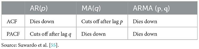
Table 1. Behavior of ACF and PACF.

In the second step, the parameters of the models identified (defined) in the first step are estimated. The maximum likelihood (ML) approach is employed in the model estimation. In a standard Gaussian, the likelihood function is given as follows:

$\begin{array}{ll}LogL=-\frac{T}{L}ln(2\pi )-\frac{T}{L}ln{\sigma }^2-\frac{1}{2{\sigma }^2}{\displaystyle \sum _{i=1}^T}{\epsilon }_t^2& (10)\end{array}$

where T is the time at t = 1, 2…, T of time series data and σ and ε are the constant variance and the error term, respectively. The logarithm of the probability of the observed data from the fitted model is shown by the log-likelihood [37]. The model with the maximum log-likelihood is chosen. To select the most appropriate ARIMA model, the Akaike Information Criterion (AIC) is applied to all competing models. The AIC proposed by Akaike [39] is a method that uses in-sample fit to determine the likelihood of a model forecasting future values [40]. The model with the lowest AIC value is the best one among all the other estimated models [41]. The equation used to estimate the AIC is as follows:

$\begin{array}{ll}AIC=-2^{*}In(L)+2^{*}k& (11)\end{array}$

where L is the value of the likelihood and k is the number of estimated parameters.

In the Box–Jenkins technique, the third step is diagnostic testing, which entails standard testing procedures on the estimations and the error terms' statistical properties (weak white noise assumption and normality assumption) [42]. The adequacy of the model can be evaluated using both formal testing techniques and graphical testing methods. The Ljung–Box [43] test will be used to check the overall acceptability of the overall model. The hypothesis for Ljung–Box is formulated as follows:

$\begin{array}{ll}{H}_0=modelisadequate& (12)\end{array}$

$\begin{array}{ll}{H}_1=modelisnotadequate& (13)\end{array}$

The test statistic for Ljung–Box is computed using the following equation:

$\begin{array}{ll}{Q}^{\ast }=n^1\left(n^1+2\right){\displaystyle \sum _{l=1}^k\frac{1}{n^1-l}{r}_l^2\left(\widehat{a}\right)}& (14)\end{array}$

where n¹ = n−d, n is the number of observations used in the estimated model and d is the level of non-seasonal differencing employed in transforming the initial time series data into stationary data. The $r_l^2(â)$ represents the square of the residual's autocorrelation at lag l. If Q^* is larger (significantly larger from zero), it is that the autocorrelation residuals are considerably distinct from 0 as a collection, and the estimated model's random shocks are autocorrelated. Since the model will be rejected, one should consider repeating the model-building cycle [30]. The Jarque–Bera test, which will be used to test the normality of the residuals of the model, is a common statistical test used to test for normality in return series. This assumption refers to the degree to which data follows a normal distribution. The JB test for normality comes from a Chi-square distribution, which is calculated using the skewness and kurtosis with two degrees of freedom. The following is the formulation of the hypothesis that will be tested:

$\begin{array}{ll}{H}_0:E({\epsilon }^2)=0(Dataisnormallydistributed)& (15)\end{array}$

$\begin{array}{ll}{H}_1:E({\epsilon }^2)\ne 0(Non-normaldistributionofdata)& (16)\end{array}$

The JB test statistic is computed using the following equation:

$\begin{array}{ll}JB=N^{*}\left[\frac{skewness}{6}+\frac{{(kurtosis-3)}^2}{4}\right]& (17)\end{array}$

where N is the number of observations. The likelihood that the given series is drawn from a normal distribution decreases with increasing JB value.

3.2 ANN-based ELM

Tokar and Johnson [44] defined ANN-based ELM as a “fast-training artificial intelligence (AI) approach for prediction that employs a Single Layer Feedforward Neural Network (SLFN) to build a relationship between complicated nonlinear dependent and independent variables”. This method has the advantage of not requiring any knowledge of the complexity of the process under study. The adoption of a nonlinear activation function and the capability of randomly learning input weights increased the popularity of this technique among researchers [45]. When training input, the layer's ANN-based ELM hidden node is independent of the hidden layer. This indicates that hidden nodes were independent of the input training set [46]. For N arbitrary distinct inputs samples (u_i, t_i), where $u={\left[u_{i1},u_{i2}\dots \dots u_{in}\right]}^T\in R^n$ and $t_i={\left[t_{i1},t_{i2}\dots \dots t_{im}\right]}^T\in R^m$. The following formula can be used to represent SLFNs with hidden neurons:

$\begin{array}{ll}{\displaystyle \sum _{i=1}^{\widehat{N}}}{\beta }_i{g}_i(u_i)={\displaystyle \sum _{i=1}^{\widehat{N}}}{\beta }_{i}g(w_i•u_j+b_i)=0_{j}j=1,\dots .,N& (18)\end{array}$

where $w_i={\left[w_{i1},w_{i2},\dots \dots ,w_{in}\right]}^T$ is the weight vector between the input nodes and the ith hidden node, β = [β_i1, β_i2, ……, β_in] is the weight vector between the ith hidden node and the output nodes, b_i denotes the threshold of the ith hidden node, and w_i•u_i is the inner product of w_i and u_i [45, 47]. The SLFN can approximate n vectors means that there exist b_i, w_i such that

$\begin{array}{ll}{\displaystyle \sum _{j=1}^{\tilde{N}}\Vert O_j-T_j\Vert }=0& (19)\end{array}$

The term β_i of Equation 18 is estimated as follows:

$\begin{array}{ll}{\displaystyle \sum _{i=1}^{\widehat{N}}}{\beta }_{i}g(w_i•u_j+b_i)=t_j,j=1\dots \dots ,N& (20)\end{array}$

Equation 20 can also be written as follows:

$\begin{array}{ll}H\beta =T,& (21)\end{array}$

where H is the hidden layer output matrix of the NNs given by

$\begin{array}{ll}H=(w_i\dots w_n,b_1\dots b_n,u_1\dots \dots u_n)=& (22)\end{array}$

$\begin{array}{ll}{\left[\begin{array}{c}g(w_1•u_1+b_1)\&\dots \&g(w_{\tilde{n}}•u_1+b_{\tilde{N}})\\ ⋮\&\cdots \&⋮\\ g(w_1•u_N+b_1)\&\cdots \&g(w_{\tilde{N}}•u_N+b_{\tilde{N}})\\ \end{array}\right]}_{N\times \tilde{N}}& (23)\end{array}$

where β is the weights connecting the hidden and output layers computed using the following:

$\begin{array}{ll}\beta ={\left[\begin{array}{c}{\beta }_1^T\\ ⋮\\ {\beta }_{\tilde{N}}^T\\ \end{array}\right]}_{\tilde{N}\times M}& (24)\end{array}$

where T is the target values of N vectors in the training dataset given by

$\begin{array}{ll}T={\left[\begin{array}{c}{t}_1^T\\ ⋮\\ t_N^T\\ \end{array}\right]}_{N\times M}& (25)\end{array}$

where H₀ is referred to as the generalized Moore-Penrose inverse of matrix H. When the number of hidden neurons and training samples is equal, SLFNs may approximate the training samples with no error. Numerous techniques, such as singular value decomposition (SVD), iterative approaches, orthogonal projection methods, and orthogonalization methods, can be used to determine H_o. It was shown that SLFNs with randomly generated hidden nodes and with a pervasive piecewise continuous activation function may universally approximate any continuous target function. The SVD approach is employed to compute H₀ [45].

3.3 Hybrid ARIMA-ANN-based ELM

The goal of hybrid models is to lower the probability of employing an incorrect model by fusing different models to lower the chance of failure and provide more accurate results [19]. The ARIMA and ANN-based ELM models have found success in their respective nonlinear or linear areas. However, none of these is a universal model that can be applied to all situations. Traditional models' approximation to complicated nonlinear issues and ANN-based ELM approximation to linear problems may be completely incorrect, especially in situations with both nonlinear and linear correlation structures. Unlike previously introduced hybrid forecasting models, which normally handle the original forecasting models as distinct linear or nonlinear units, the suggested hybrid model is an integrated model that can respond well to both linear and nonlinear conditions, which are common in complex frequent time series.

According to a few researchers in hybrid linear and nonlinear models, it would be reasonable to assume that a time series is made up of a linear autocorrelation structure and a nonlinear component [48], which is given as follows:

$\begin{array}{ll}{y}_t=N_t+L_t& (26)\end{array}$

where L_t represents the linear component and N_t represents the nonlinear component. The data must be used to estimate these two components. The study first allows ARIMA to model the linear component, and only the nonlinear relationship will be present in the residuals from the linear model [48]. Let e_t represent the residual at time t from the linear model, then

$\begin{array}{ll}{e}_t=y_t-{\widehat{L}}_t& (27)\end{array}$

where ${\widehat{L}}_t$ is the forecast value for time t from the estimated relationship. By modeling the residuals using ANN-based ELM, the nonlinear relationship can be revealed [48]. With n input nodes, the ANN-based ELM model for the residuals will be as follows:

$\begin{array}{ll}{e}_t=f(e_{t-1},\dots ,e_{t-n})+{\epsilon }_t& (28)\end{array}$

where f is the nonlinear function that is established by the NN and e_t is the random error. It should be noted that the error term may not be random if the model f is inappropriate [48]. Consequently, it is crucial to identify the right model. The forecast from Equation 28 is represented as ${\widehat{N}}_t$, then the combined forecast will be as follows:

$\begin{array}{ll}{ŷ}_t={\widehat{L}}_t+{\widehat{N}}_t& (29)\end{array}$

The hybrid model uses the unique characteristics and strengths of both the ANN-based ELM and the ARIMA models to identify various patterns. To improve the overall effectiveness of modeling and forecasting, it may be useful to model linear and nonlinear patterns independently using several models before combining the forecasts [48, 49]. The flowchart of the hybrid model is presented in Figure 1.

Figure 1

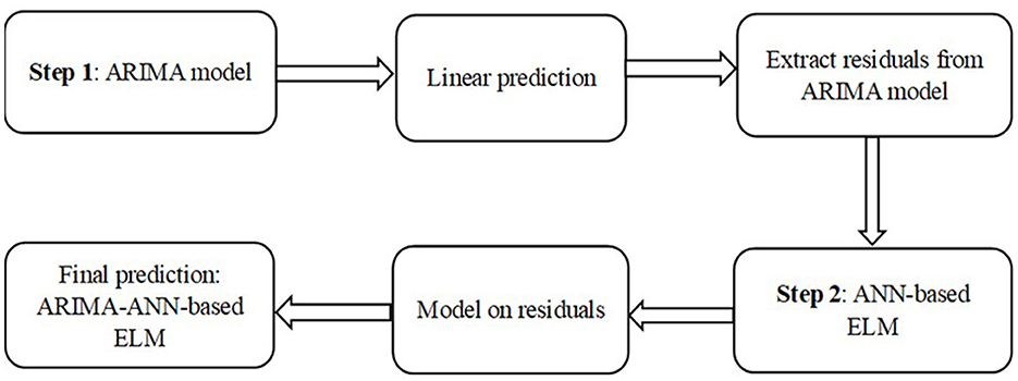
Figure 1. The flowchart of the hybrid model.

3.4 Model evaluation

Three evaluation metrics, such as MAPE, MSE, and MAE, are employed to measure the predictability of the methods, which are computed from the following equations:

$\begin{array}{ll}MAPE=\frac{1}{N}{\displaystyle \sum _{i=t}^N}\frac{|x_i-{\widehat{x}}_i|}{\left|x_i\right|}\times 100\%& (30)\end{array}$

$\begin{array}{ll}MSE=\frac{1}{\overline{N}}{\displaystyle \sum _{i=1}^N}{(x_i-{\widehat{x}}_i)}^2& (31)\end{array}$

$\begin{array}{ll}MAE=\frac{1}{N}{\displaystyle \sum _{i=t}^N}\frac{|x_i-{\widehat{x}}_i|}{\left|x_i\right|}& (32)\end{array}$

where n is the number of values and $\widehat{x}$ is the forecast value [50]. The model with the lowest values of MAPE, MSE, and MAE will be selected and proposed as an adequate algorithm for predicting purposes.

4 Results and discussion

This section of the study presents the results of the data analysis and the discussion of the results obtained from the data analysis. Table 2 presents the results of the descriptive statistics. Descriptive statistics are used to describe the dataset used in the study. The results in Table 2 revealed that both the mean and median are positive, suggesting that the closing prices increase slightly over time. The skewness coefficient shows that time series data is skewed to the right. A negative kurtosis demonstrates that the distribution is relatively flat. The kurtosis value of the time series data is less than 3, which reveals that the distribution has characteristics of a platykurtic distribution. The standard deviation value is 8,751.866, and this large value suggests that the data points are more spread apart from the mean. This signifies that the time series data has a higher level of variability or dispersion.

Table 2

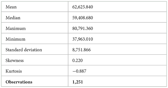
Table 2. The results of the descriptive statistics of JSE/FTSE closing prices.

4.1 The findings from the Box–Jenkins procedure

The Box–Jenkins procedure used in the study follows a three-step approach. The three-step approach is outlined in the following subsections.

4.1.1 Model identification

To create a BJ model, first determine whether the series is stationary and observe any patterns. The plot provides a first indication of the expected nature of the time series as presented in Figure 2.

Figure 2

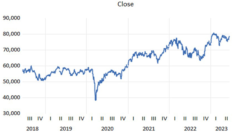
Figure 2. Time series plot of JSE/FTSE closing prices.

The time series plot of JSE/FTSE closing prices is presented above in Figure 2. The plot reveals irregular fluctuations, which implies that the mean and variance change over time. This is a demonstration that this time series is non-stationary by eye inspection. Through logarithm differencing, trend behavior in non-stationary data may be changed. As stated, this study places a greater emphasis on logarithmic differencing. In any time series study, it is significant to understand the concept of stationarity and its definition regarding keeping statistical properties constant over time. The stationarity test makes the study of model estimation and forecasts easier. The study made use of ADF and KPSS tests.

The stationary test results for ADF and KPSS are presented in Table 3. The null hypothesis of a unit root (non-stationary series) is not rejected, since the p-value associated with the ADF test is greater than the 5% significance level. This indicates that the time series is not stationary and has a trend or other types of dependency over time. Furthermore, the KPSS test findings have a p-value less than the significant level of 5%, the null hypothesis is rejected, and the time series data is non-stationary. Both tests provide evidence that differencing/logarithm is necessary. The results of the ADF test indicate that the time series is stationary after log differencing since its p-value is less than the 5% significance level, thus rejecting the null hypothesis of non-stationary. The KPSS results are also consistent with the ADF test results, which also provide evidence that, at a 5% significance level, the log-differenced time series is indeed stationary. The time series plot of the log-differenced data is presented in Figure 3.

Table 3

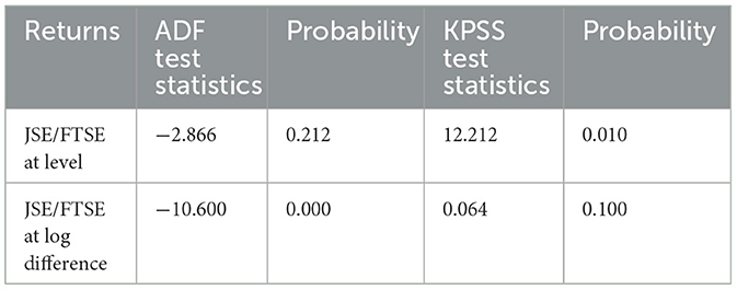
Table 3. ADF and KPSS test results of JSE/FTSE closing prices.

Figure 3

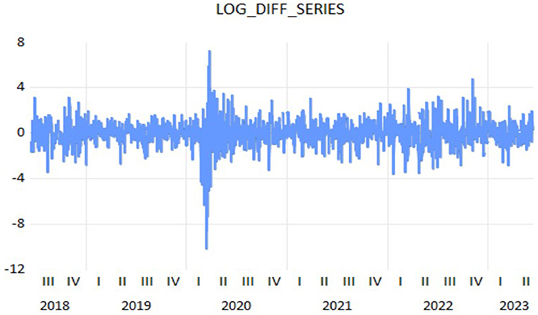
Figure 3. Time series plot of the log differenced data.

The figure shows fluctuation around the mean of zero, suggesting that the series remains constant to the mean. In addition to graphical stationarity checking, the ACF and PACF are employed for formal testing and identify the order of ARIMA models.

Considering Figure 4 of the ACF and PACF plots, it is observed that the PACF plot suggests AR [6] and AR [7]. The ACF plot also suggests MA [6] and MA [7]. In the ACF plot, spikes are additionally observed at higher lags. The strikes from lag 8 have been discarded since Tsoku et al. (42, p. 764) specified that “spikes at greater lags are commonly ignored to simplify the initial tentatively recognized model.” The plots indicated several AR and MA lags; therefore, the AIC approach will be employed as the selection criteria to select an ARIMA model.

Figure 4

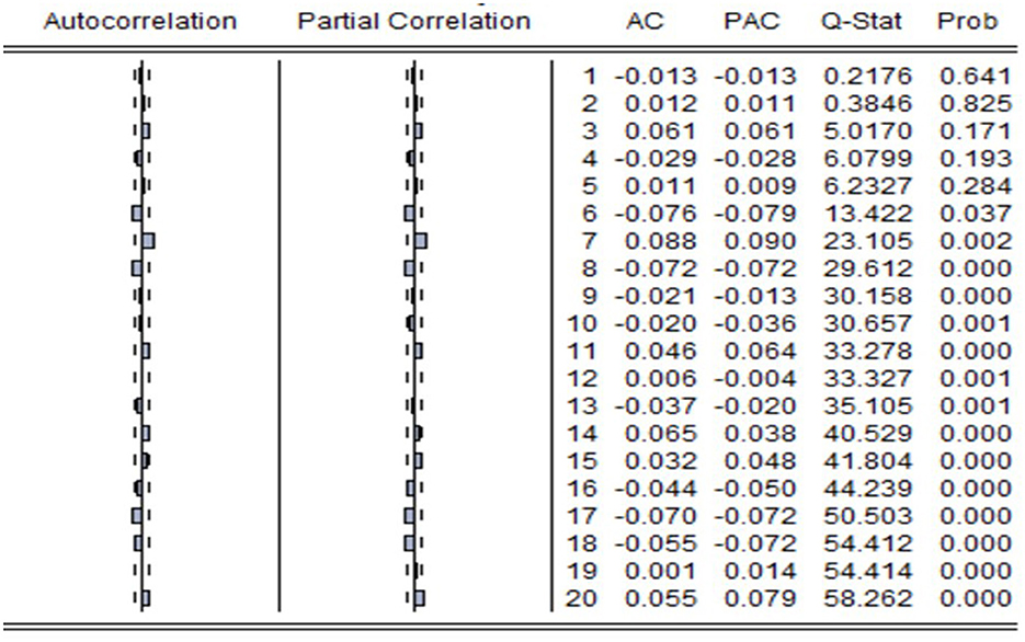
Figure 4. ACF and PACF plots of the log differenced data.

4.1.2 Model estimation and selection

The findings indicated the existence of ARIMA models with various lag orders. However, not all the ARIMA models found could be used in this study. Hence, choosing an appropriate model is crucial. Table 4 gives a summary of the models that are compared. According to the findings in Table 5, the chosen ARIMA model for log-differenced data is ARIMA [1, 6, 6] based on the lowest AIC value. The findings further revealed that ARIMA [1, 6, 7] did not converge, therefore the model was not considered. The next step is to compute the parameter estimation of the selected model. The results presented in Table 5 show the coefficients of AR and MA components that resulted from modeling the selected model using the ML method.

Table 4

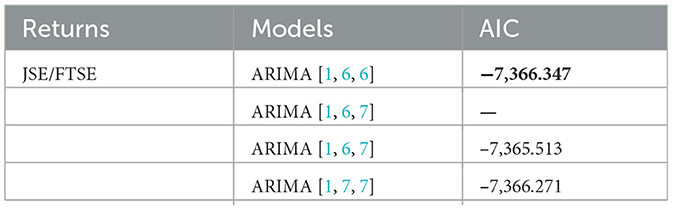
Table 4. Model selection of ARIMA models for log-differenced data.

Table 5

Table 5. Parameter estimates of fitted ARIMA [1, 6, 6].

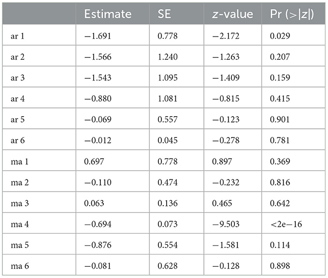
Based on the coefficients summarized in Table 5, the estimated parameters generate the following equation:

$\begin{array}{l}{Y}_t=-1.691Y_{t-1}-1.566Y_{t-2}-1.543Y_{t-3}-0.880Y_{t-4}\\ -0.069Y_{t-5}-0.0123Y_{t-6}+0.697e_{t-1}-0.110e_{t-2}\\ +0.063e_{t-3}-0.6940e_{t-4}-0.876e_{t-5}-0.081e_{t-6}+{\epsilon }_t& (33)\end{array}$

The next step is to run a diagnostic check to ensure that the chosen model is appropriate for further analysis.

4.1.3 Diagnostic checking results

The best-fit model is determined by how well the residual analysis is carried out in time series modeling [51]. The diagnostic test results of the fitted ARIMA model are presented in Tables 6, 7 and Figures 5, 6.

Table 6

Table 6. JB test results of the fitted ARIMA [1, 6, 6] model residuals.

Table 7

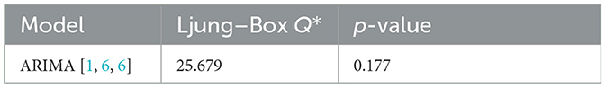
Table 7. Diagnostic test results of the fitted ARIMA model residuals.

Figure 5

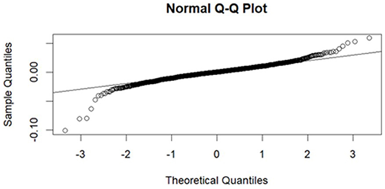
Figure 5. Q-Q plot of the fitted ARIMA model residuals.

Figure 6

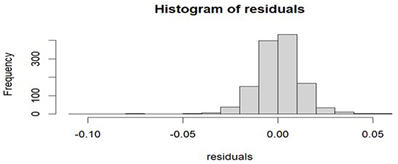
Figure 6. Histogram of the fitted ARIMA model residuals.

The JB test was employed to determine the normality of the residuals, and the findings are shown in Table 6. The findings suggest that the null hypothesis of normality in the residuals is not accepted, and the conclusion is that the residual distribution is not normal. The graphical representations of residual diagnostics are displayed in Figures 5, 6. It is evident from Figure 5 that almost all the points are either on the 45-degree line or very near to it, but a few of the points are slightly separated from the Quantile-Quantile (QQ) line. Furthermore, the residuals of the fitted model are slightly negatively skewed and normally distributed, as shown by the histogram in Figure 6.

To further test the model's adequacy, this study performed the Ljung–Box test for residuals. The Q^* statistic (25.679) of the residuals and p-value (0.177) are given in Table 7, where the null hypothesis is not rejected since the p-value exceeds the significant level of 5%. Therefore, it can be concluded that there is sufficient statistical evidence that the selected model is adequate. This suggests that the fitted ARIMA [1, 6, 6] model is sufficient enough to be used for further analysis.

4.2 ANN-based ELM

As the second step of the analysis, ANN-based ELM was applied. The dataset was divided into test data and training data to assess the forecasting abilities of the model. The test data is used to assess the forecasted model, while the training data is used to build the model. The dataset was split into 80% training and 20% testing. The log-differenced data set has test and train sizes of 250 and 1,000 rows, respectively. With an 80%/20% splitting approach, predictive models can obtain better prediction performance, as outlined by Abdulkareem et al. [52]. The model is trained using the training data set, and then the test dataset is used to assess its performance. The study evaluated the model's performance using three evaluation metrics, and the results are presented in Table 8.

Table 8

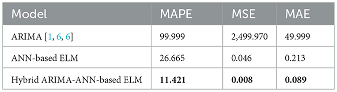
Table 8. Evaluation metrics for the differenced data.

4.3 Hybrid ARIMA-ANN-based ELM

Different ARIMA models were obtained for the initial step of building hybrid models in ARIMA-ANN-based ELM modeling, but for better results, the log-differenced data were fitted using the ARIMA [1, 6, 6] model. The hybrid model was performed by modeling the residuals from the ARIMA [1, 6, 6] model using an ANN-based ELM. The accuracy measurements, to show which model was chosen, were used to determine which model can be used for forecasting between ARIMA[1, 6, 6], ANN-based ELM, and hybrid ARIMA-ANN-based ELM, and the results are provided in Table 8. The results in Table 8 indicate that the hybrid ARIMA-ANN-based ELM yields better prediction results for closing prices since it has the lowest values of MAPE, MSE, and MAE. Therefore, the hybrid ARIMA-ANN-based ELM was selected as a better-performing model as compared to the individual models.

5 Conclusion

The study modeled the closing stock prices using three models, namely, ARIMA, ANN-based ELM, and a hybrid of ARIMA-ANN-based ELM to determine the most appropriate model. The findings demonstrated that there were four competing ARIMA models, namely, ARIMA [1, 6, 6], ARIMA [1, 6, 7], ARIMA [1, 6, 7], and ARIMA [1, 7, 7]. The chosen ARIMA model for log-differenced data was found to be ARIMA [1, 6, 6] based on the lowest AIC value.

The diagnostic test was computed and revealed that the chosen model was adequate. The dataset was then divided into 80% for training and 20% for testing for ANN-based ELM. The model was trained using the training data set, and its performance was evaluated using the test dataset. These methods, however, may not be sufficient when modeling time series data with both linear and nonlinear characteristics simultaneously, as stated by Bulut and Hudaverdi [53]. Hence, this study proposed a hybrid of both ARIMA and ANN-based ELM to model both linearity and nonlinearity simultaneously. The study developed a hybrid approach for time series prediction that aims to address the limitations of prior hybrid methods by eliminating strong assumptions. It was evident from the findings that the hybrid model performed better than the individual models. It was also evident that the hybrid model improved the performance of the ARIMA and ANN-based ELM when computed individually.

The study by Khan et al. [54] also integrated the ARIMA and ANN models. The findings from the study by Khan et al. [54] demonstrated that ANN performs more effectively in forecasting than the ARIMA model, but when their forecasts are combined, the hybrid ARIMA-ANN outperformed in terms of forecast accuracy, ANN, and ARIMA. The study recommends policymakers and practitioners to use the hybrid model as it yields better results. In the future, researchers may delve into assessing the effectiveness of models by using additional conventional linear models and hybrid variants such as ARIMA-GARCH and ARIMA-EGARCH. Future studies could also integrate these with nonlinear models to better capture both linear and nonlinear patterns in the data. This approach offers a promising avenue for enhancing model performance and gaining deeper insights into complex phenomena.

Data availability statement

Publicly available datasets were analyzed in this study. This data can be found at: Johannesburg Stock Exchange (jse.co.za).

Author contributions

OM: Writing – original draft, Writing – review & editing. JT: Writing – original draft, Writing – review & editing. DM: Writing – original draft, Writing – review & editing.

Funding

The author(s) declare that no financial support was received for the research, authorship, and/or publication of this article.

Acknowledgments

The authors are grateful to the JSE for providing the necessary data.

Conflict of interest

The authors declare that the research was conducted in the absence of any commercial or financial relationships that could be construed as a potential conflict of interest.

Publisher's note

All claims expressed in this article are solely those of the authors and do not necessarily represent those of their affiliated organizations, or those of the publisher, the editors and the reviewers. Any product that may be evaluated in this article, or claim that may be made by its manufacturer, is not guaranteed or endorsed by the publisher.

References

1. Box GE, Jenkins GM. Time Series Analysis: Forecasting and Control. San Francisco, CA: Holden-Day (1976).

Google Scholar

2. Engle RF. Autoregressive conditional heteroscedasticity with estimates of the variance of United Kingdom inflation. Econometrica (1982) 987–1007. doi: 10.2307/1912773

Crossref Full Text | Google Scholar

3. Bollerslev T. Generalized autoregressive conditional heteroskedasticity. J Econom. (1986) 31:307–27. doi: 10.1016/0304-4076(86)90063-1

Crossref Full Text | Google Scholar

4. Zhao Y, Chen Z. Forecasting stock price movement: new evidence from a novel hybrid deep learning model. J Asian Bus Econ Stud. (2022) 29:91–104. doi: 10.1108/JABES-05-2021-0061

Crossref Full Text | Google Scholar

5. Mirzavand M, Ghazavi R. A stochastic modelling technique for groundwater level forecasting in an arid environment using time series methods. Water Resour Manag. (2015) 29:1315–28. doi: 10.1007/s11269-014-0875-9

Crossref Full Text | Google Scholar

6. Box GE, Jenkins GM, MacGregor JF. Some recent advances in forecasting and control. J R Stat Soc C Appl Stat. (1974) 23:158–79. doi: 10.2307/2346997

Crossref Full Text | Google Scholar

7. Madge S, Bhatt S. Predicting Stock Price Direction using Support Vector Machines. Independent work report Spring. (2015), p. 45.

PubMed Abstract | Google Scholar

8. Chen Y, Hao Y. A feature weighted support vector machine and K-nearest neighbor algorithm for stock market indices prediction. Expert Syst Appl. (2017) 80:340–55. doi: 10.1016/j.eswa.2017.02.044

Crossref Full Text | Google Scholar

9. Xie Y, Jiang H. Stock market forecasting based on text mining technology: a support vector machine method. arXiv. (2019) [Preprint]. arXiv:1909.12789. doi: 10.48550/arXiv.1909.12789

Crossref Full Text | Google Scholar

10. Wanjawa BW, Muchemi L. ANN model to predict stock prices at stock exchange markets. arXiv. (2014) [Preprint]. arXiv:1502.06434. doi: 10.48550/arXiv.1502.06434

Crossref Full Text | Google Scholar

11. Gurjar M, Naik P, Mujumdar G, Vaidya T. Stock market prediction using ANN. Int Res J Eng Technol. (2018) 5:2758–61.

Google Scholar

12. Devadoss AV, Ligori TAA. Stock prediction using artificial neural networks. Int J Data Min Tech. Appl. (2013) 2:283–91.

Google Scholar

13. Liu X, He P, Chen W, Gao J. Multi-task deep neural networks for natural language understanding. arXiv. (2019) [Preprint]. arXiv:1901.11504. doi: 10.48550/arXiv.1901.11504

Crossref Full Text | Google Scholar

14. Rezaei H, Faaljou H, Mansourfar G. Stock price prediction using deep learning and frequency decomposition. Expert Syst Appl. (2021) 169:114332. doi: 10.1016/j.eswa.2020.114332

Crossref Full Text | Google Scholar

15. Kamalov F, Cherukuri AK, Sulieman H, Thabtah F, Hossain A. Machine learning applications for COVID-19: a state-of-the-art review. Data Sci Genomics. (2023) 277–89. doi: 10.1016/B978-0-323-98352-5.00010-0

Crossref Full Text | Google Scholar

16. Tung TM, Yaseen ZM. A survey on river water quality modelling using artificial intelligence models: 2000–2020. J. Hydrol. (2020) 585:124670. doi: 10.1016/j.jhydrol.2020.124670

Crossref Full Text | Google Scholar

17. de Julián-Ortiz JV, Pogliani L, Besalú E. Modeling properties with artificial neural networks and multilinear least-squares regression: advantages and drawbacks of the two methods. Appl Sci. (2018) 8:1094. doi: 10.3390/app8071094

Crossref Full Text | Google Scholar

18. Ahmad AS, Hassan MY, Abdullah MP, Rahman HA, Hussin F, Abdullah H, et al. A review on applications of ANN and SVM for building electrical energy consumption forecasting. Renew Sustain Energy Rev. (2014) 33:102–9. doi: 10.1016/j.rser.2014.01.069

Crossref Full Text | Google Scholar

19. Khashei M, Bijari M. A novel hybridization of artificial neural networks and ARIMA models for time series forecasting. Appl Soft Comput. (2011) 11:2664–75. doi: 10.1016/j.asoc.2010.10.015

Crossref Full Text | Google Scholar

20. Cerjan M, KrŽelj I, Vidak M, Delimar M. A literature review with statistical analysis of electricity price forecasting methods. Eurocon. (2013) 2013:756–63. doi: 10.1109/EUROCON.2013.6625068

Crossref Full Text | Google Scholar

21. Zhou C, Yin K, Cao Y, Ahmed B, Fu X. A novel method for landslide displacement prediction by integrating advanced computational intelligence algorithms. Sci Rep. (2018) 8:7287. doi: 10.1038/s41598-018-25567-6

PubMed Abstract | Crossref Full Text | Google Scholar

22. Barzegar R, Fijani E, Moghaddam AA, Tziritis E. Forecasting of groundwater level fluctuations using ensemble hybrid multi-wavelet neural network-based models. Sci Total Environ. (2017) 599:20–31. doi: 10.1016/j.scitotenv.2017.04.189

PubMed Abstract | Crossref Full Text | Google Scholar

23. Manssouri I, Boudebbouz B, Boudad B. Using artificial neural networks of the type extreme learning machine for the modelling and prediction of the temperature in the head the column. Case of a C6H11-CH3 distillation column. Mater Today Proc. (2021) 45:7444–9. doi: 10.1016/j.matpr.2021.01.920

Crossref Full Text | Google Scholar

24. Milačić L, Jović S, Vujović T, Miljković J. Application of artificial neural network with extreme learning machine for economic growth estimation. Phys A: Stat Mech Appl. (2017) 465:285–8. doi: 10.1016/j.physa.2016.08.040

Crossref Full Text | Google Scholar

25. Khan S, Alghulaiakh H. ARIMA model for accurate time series stocks forecasting. Int J Adv Comput Sci Appl. (2020) 11. doi: 10.14569/IJACSA.2020.0110765

Crossref Full Text | Google Scholar

26. Khanderwal S, Mohanty D. Stock price prediction using ARIMA model. Int J Mark Hum Resour Res. (2021) 2:98–107.

Google Scholar

27. Pan F, Zhang H, Xia M. A hybrid time series forecasting model using extreme learning machines. In: 2009 Second International Conference on Intelligent Computation Technology and Automation, Vol. 1. Changsha: IEEE (2009), 933–936. doi: 10.1109/ICICTA.2009.232

Crossref Full Text | Google Scholar

28. Büyükşahin ÜÇ, Ertekin S. Improving forecasting accuracy of time series data using a new ARIMA-ANN hybrid method and empirical mode decomposition. Neurocomputing. (2019) 361:151–63. doi: 10.1016/j.neucom.2019.05.099

Crossref Full Text | Google Scholar

29. Box G, Jenkins G. Time Series Analysis-Forecasting and Control. San Francisco, CA: Holden Day (1970), p. 553.

Google Scholar

30. Hamjah MA. Forecasting major fruit crops productions in Bangladesh using Box-Jenkins ARIMA model. J Econ Sustain Dev. (2014) 5.

Google Scholar

31. Wang L, Zou H, Su J, Li L, Chaudhry S. An ARIMA-ANN hybrid model for time series forecasting. Syst Res Behav Sci. (2013) 30:244–59. doi: 10.1002/sres.2179

PubMed Abstract | Crossref Full Text | Google Scholar

32. Carvajal TM, Viacrusis KM, Hernandez LFT, Ho HT, Amalin DM, Watanabe K. Machine learning methods reveal the temporal pattern of dengue incidence using meteorological factors in metropolitan Manila, Philippines. BMC Infect Dis. (2018) 18:1–15. doi: 10.1186/s12879-018-3066-0

PubMed Abstract | Crossref Full Text | Google Scholar

33. Siami-Namini S, Tavakoli N, Namin AS. A comparison of ARIMA and LSTM in forecasting time series. In: 2018 17th IEEE international conference on machine learning and applications (ICMLA). Orlando, FL: IEEE (2018), p. 1394401. doi: 10.1109/ICMLA.2018.00227

Crossref Full Text | Google Scholar

34. Dickey DA, Fuller WA. Distribution of the estimators for autoregressive time series with a unit root. J Am Stat Assoc. (1979) 74:427–31. doi: 10.1080/01621459.1979.10482531

Crossref Full Text | Google Scholar

35. Kwiatkowski D, Phillips PC, Schmidt P, Shin Y. Testing the null hypothesis of stationarity against the alternative of a unit root: how sure are we that economic time series have a unit root? J Econom. (1992) 54:159–78. doi: 10.1016/0304-4076(92)90104-Y

Crossref Full Text | Google Scholar

36. Imam A, Habiba D, Atanda BT. On consistency of tests for stationarity in autoregressive and moving average models of different orders. Am J Theor Appl Stat. (2016) 5:146–53. doi: 10.11648/j.ajtas.20160503.20

Crossref Full Text | Google Scholar

37. Mohamed J. Time series modeling and forecasting of Somaliland consumer price index: a comparison of ARIMA and regression with ARIMA errors. Am J Theor Appl Stat. (2020) 9:143–53. doi: 10.11648/j.ajtas.20200904.18

Crossref Full Text | Google Scholar

38. Islam MR, Nguyen N. Comparison of financial models for stock price prediction. J Risk Financial Manag. (2020) 13:181. doi: 10.3390/jrfm13080181

Crossref Full Text | Google Scholar

39. Akaike H. A new look at the statistical model identification. IEEE Trans Automat Contr. (1974) 19:716–23. doi: 10.1109/TAC.1974.1100705

Crossref Full Text | Google Scholar

40. Tran DA, Tsujimura M, Ha NT, Van Binh D, Dang TD, Doan QV, et al. Evaluating the predictive power of different machine learning algorithms for groundwater salinity prediction of multi-layer coastal aquifers in the Mekong Delta, Vietnam. Ecol Indic. (2021) 127:107790. doi: 10.1016/j.ecolind.2021.107790

Crossref Full Text | Google Scholar

41. Velasco JA, González-Salazar C. AIC should not be a “test” of geographical prediction accuracy in ecological niche modelling. Ecol Inform. (2019) 51:25–32. doi: 10.1016/j.ecoinf.2019.02.005

Crossref Full Text | Google Scholar

42. Tsoku JT, Phukuntsi N, Metsileng D. Gold sales forecasting: the Box–Jenkins methodology. Risk Gov Control Financ Mark Inst. (2017) 7:54–60. doi: 10.22495/rgcv7i1art7

Crossref Full Text | Google Scholar

43. Ljung GM, Box GE. On a measure of lack of fit in time series models. Biometrika. (1978) 65:297–303. doi: 10.1093/biomet/65.2.297

Crossref Full Text | Google Scholar

44. Tokar AS, Johnson PA. Rainfall-runoff modeling using artificial neural networks. J Hydrol Eng. (1999) 4:232–9. doi: 10.1061/(ASCE)1084-0699(1999)4:3(232)

Crossref Full Text | Google Scholar

45. Sahoo BB, Jha R, Singh A, Kumar D. Application of support vector regression for modeling low flow time series. KSCE J Civil Eng. (2019) 23:923–34. doi: 10.1007/s12205-018-0128-1

PubMed Abstract | Crossref Full Text | Google Scholar

46. Lei Y, Zhao D, Cai H. Prediction of length-of-day using extreme learning machine. Geod Geodyn. (2015) 6:151–9. doi: 10.1016/j.geog.2014.12.007

Crossref Full Text | Google Scholar

47. Utomo CP. The hybrid of classification tree and extreme learning machine for permeability prediction in oil reservoir. Int J Comput Sci Issues. (2013) 11:10:52.

Google Scholar

48. Zhang GP. Time series forecasting using a hybrid ARIMA and neural network model. Neurocomputing. (2003) 50:159–75. doi: 10.1016/S0925-2312(01)00702-0

Crossref Full Text | Google Scholar

49. Adhikari R, Agrawal RK. Performance evaluation of weights selection schemes for linear combination of multiple forecasts. Artif Intell Rev. (2014) 42:529–48. doi: 10.1007/s10462-012-9361-z

PubMed Abstract | Crossref Full Text | Google Scholar

50. Hong YY, Rioflorido CLPP. A hybrid deep learning-based neural network for 24-h ahead wind power forecasting. Appl Energy. (2019) 250:530–9. doi: 10.1016/j.apenergy.2019.05.044

Crossref Full Text | Google Scholar

51. Unhapipat S. ARIMA model to forecast international tourist visit in Bumthang, Bhutan. J Phys Conf Ser. (2018) 1039:012023. doi: 10.1088/1742-6596/1039/1/012023

Crossref Full Text | Google Scholar

52. Abdulkareem KH, Mohammed MA, Salim A, Arif M, Geman O, Gupta D, et al. Realizing an effective COVID-19 diagnosis system based on machine learning and IOT in smart hospital environment. IEEE Internet Things J. (2021) 8:15919–28. doi: 10.1109/JIOT.2021.3050775

PubMed Abstract | Crossref Full Text | Google Scholar

53. Bulut C, Hudaverdi B. Hybrid approaches in financial time series forecasting: a stock market application. Ekoist J Econ Stat. (2022) 37:53–68. doi: 10.26650/ekoist.2022.37.1108411

Crossref Full Text | Google Scholar

54. Khan F, Urooj A, Muhammadullah S. An ARIMA-ANN hybrid model for monthly gold price forecasting: empirical evidence from Pakistan. Pak Econ Rev. (2021) 4:61–75.

Google Scholar

55. Suwardo W, Napiah M, Kamaruddin I. ARIMA models for bus travel time prediction. J Inst Eng Malaysia. (2010) 4:49–58.

Google Scholar