Quantifying impact of correlated predictors on low-cost sensor PM2.5 data using KZ filter

PM_2.5, fine particulate matter with a diameter smaller than 2.5 μm, is associated with a range of health problems. Monitoring PM_2.5 levels at the community scale is crucial for understanding personal exposure and implementing preventive measures. While monitoring agencies around the world, such as the U.S. Environmental Protection Agency (EPA), provide accurate data, the spatial coverage is limited due to a sparse monitoring network. Recently, the emergence of low-cost air quality sensor networks has enabled the availability of air quality data with higher spatiotemporal resolution, which is more representative of personal exposure. However, concerns persist regarding the sensitivity, noise, and reliability of data from these low-cost sensors. In this study, we analyzed PM_2.5 data from both EPA and Purple Air (PA) sensors in Cook County, Illinois, with two primary goals: (1) understanding the differential impact of meteorological factors on PA and EPA sensor networks and (2) provide a mathematical approach to quantify the individual impact of correlated predictors on both short-term and baseline variations in noisy time series data. We used the Kolmogorov-Zurbenko (KZ) filter to separate the time series into short-term and baseline components, followed by fitting linear models to quantify the impact of meteorological predictors, including temperature, relative humidity (RH), wind speed (WS), and wind direction (WD). Furthermore, we applied the Lindeman, Merenda, and Gold (LMG) method to these linear models to quantify the individual contribution of each predictor in the presence of multicollinearity. Our results show that the PM_2.5 data from PA sensors exhibit higher sensitivity to meteorological factors, particularly wind speed, in the short-term and RH in the baseline component. This method provides a structured approach for analyzing noisy sensor data under diverse environmental conditions.

1 Introduction

Air pollution is one of the most significant public health concerns of our era as it impacts not only public and individual health but also climate change. PM_2.5 is an air pollutant that is associated with several health risks. Microorganisms in PM_2.5 may directly cause mononuclear inflammation or disrupt microbial balance contributing to the development and exacerbation of chronic obstructive pulmonary disease (COPD) [1, 2]. Recent studies have also shown that PM_2.5 exposure is positively associated with lung cancer, COVID-19 infection, and mortality [3–7]. Understanding the impacts of air pollution at the community level can aid in informed decision-making on a larger scale.

Air monitoring is typically performed using reference monitors. In the United States, the Environmental Protection Agency (EPA) manages Air Quality Monitoring Stations (AQMSs) to monitor regulated pollutants, including ambient PM_2.5. However, these instruments are expensive and require substantial infrastructure and maintenance. Despite the availability of over a few thousand AQMSs across the U.S., the spatial coverage of this monitoring network remains sparse. When aggregating concentrations, it is often assumed that exposure to air pollution is uniform within defined areas. Consequently, this assumption induces exposure measurement errors in epidemiological studies. These errors often lead to inaccuracies, generally biasing effect estimates toward the null, thereby diminishing the apparent strength of associations [8, 9].

For precise exposure assessment and more accurate personal exposure, a high-resolution air quality monitoring network is essential. One such network that exists globally is the PurpleAir (PA) sensor network [10]. The sensing technology used in these sensors is based on laser light scattering techniques, consisting of a pair of Plantower PMS 5003 low-cost sensors that measure ambient aerosol concentrations. The PMS 5003 measures various particle concentration metrics, including PM₁, PM_2.5, and PM₁₀ [11]. However, PM sensors employed in low-cost monitors exhibit biases and calibration dependencies, especially under varying meteorological conditions. In particular, it has been established that PA low-cost sensors are sensitive to meteorological parameters, especially relative humidity (RH) [12, 13]. PA sensors tend to overestimate PM_2.5 concentrations. To address this issue, a U.S.-wide correction model for PA sensors was recently developed [12]. These models rely solely on RH and temperature as correction parameters. However, [14] found that both models tend to underestimate short-term changes in PA PM_2.5 data.

The widely used standard, U.S.-wide correction equation for PA sensor data is linear, with RH as the correction factor due to its simplicity and interpretability. Recent studies analyzing the performance of low-cost air quality sensors have noted the influence of wind speed and direction on PM_2.5 concentrations, particularly during rare events such as haze and wildfires, as well as in conditions of low and high wind speeds [13, 15, 16]. However, a limited number of studies [15, 17, 18] have focused on wind speed's impact on low-cost sensor data, primarily relying on visual inspection and simulations, without adequately addressing multicollinearity, an issue caused by correlations between weather variables like temperature, relative humidity, wind speed, and wind direction. This creates a gap in understanding how individual weather variables contribute to PM_2.5 concentrations in noisy time series data, particularly when using a linear model. Therefore, there is still a need for a technique that can systematically quantify the impact of individual variables in a linear model while addressing both short-term and baseline variations in noisy data and mitigating the effect of multicollinearity.

In this study, we introduce a mathematical technique that fills this gap by utilizing the Kolmogorov-Zurbenko (KZ) filter, in combination with the Lindeman, Merenda, and Gold (LMG) method. The KZ filter decomposes the time series into short-term and baseline components, enabling clearer identification of short-term fluctuations and long-term trends. The LMG method quantifies the relative contribution of each correlated variable, helping to disentangle the influence of temperature, relative humidity, wind speed, and wind direction, which are often correlated in air pollution models. By applying these two complementary techniques, our approach systematically analyzes the effects of individual predictors in a linear model, making it particularly useful for high temporal resolution data. This offers a clearer understanding of both short-term and baseline PM_2.5 variations in noisy datasets and, more importantly, addresses the challenge of multicollinearity, which has been largely overlooked in previous studies. The proposed technique is particularly applicable to datasets from environmental monitoring sensors including sensors for other pollutants such as Nitrogen Dioxide (NO₂), and Ozone (O₃). It helps in quantifying the impact of correlated predictors on sensor measurements to improve sensor data quality.

For the case study, we selected Cook County, IL, a significant transportation and industrial hub with major rail and road networks. We used the KZ filter to analyze short-term and baseline PM_2.5 trends in both networks and employed the LMG method to quantify the individual influence of meteorological factors. By combining the KZ filter and the LMG method, we analyzed and quantified each meteorological factor's impact on the accuracy of low-cost sensor PM_2.5 measurements in both short-term and baseline components of the time series. Our findings suggest that meteorological conditions have a higher impact on both short-term and baseline PA PM_2.5 than the EPA data. Particularly, wind speed affects the short-term and RH baseline variations of PA PM_2.5.

2 Materials and methods

2.1 Data collection and pre-processing

This study uses the publicly available hourly PM_2.5 data consisting of 2 years of EPA and PA measurements from October 2019 to September 2021 [10, 19]. The hourly averages were then converted to 24-h averages for this analysis. We collected meteorological data from five nearby stations of the National Oceanic and Atmospheric Administration (NOAA), [20] with a distance of each nearest EPA, PA sensor, and NOAA station. The meteorological variables include temperature, relative humidity (RH), wind speed (WS), and wind direction (WD). The information on these EPA, PA sampling can be extracted from Figure 1 and from supplementary of [14], the information on NOAA sites can be extracted from Supplementary Table S1. For consistency and validation of results with [12, 14], the PM_2.5 data range was set to be [1,70] μg/m³. Furthermore, the monitoring locations of EPA and PA are plotted on the map with the population density, and housing units around the sampling locations in Figure 1. The total population, housing units, and median housing income were calculated in the census blocks, as defined by the U.S. Census Bureau [38]. The PA sensors are located in urban areas with higher populations and incomes.

Figure 1

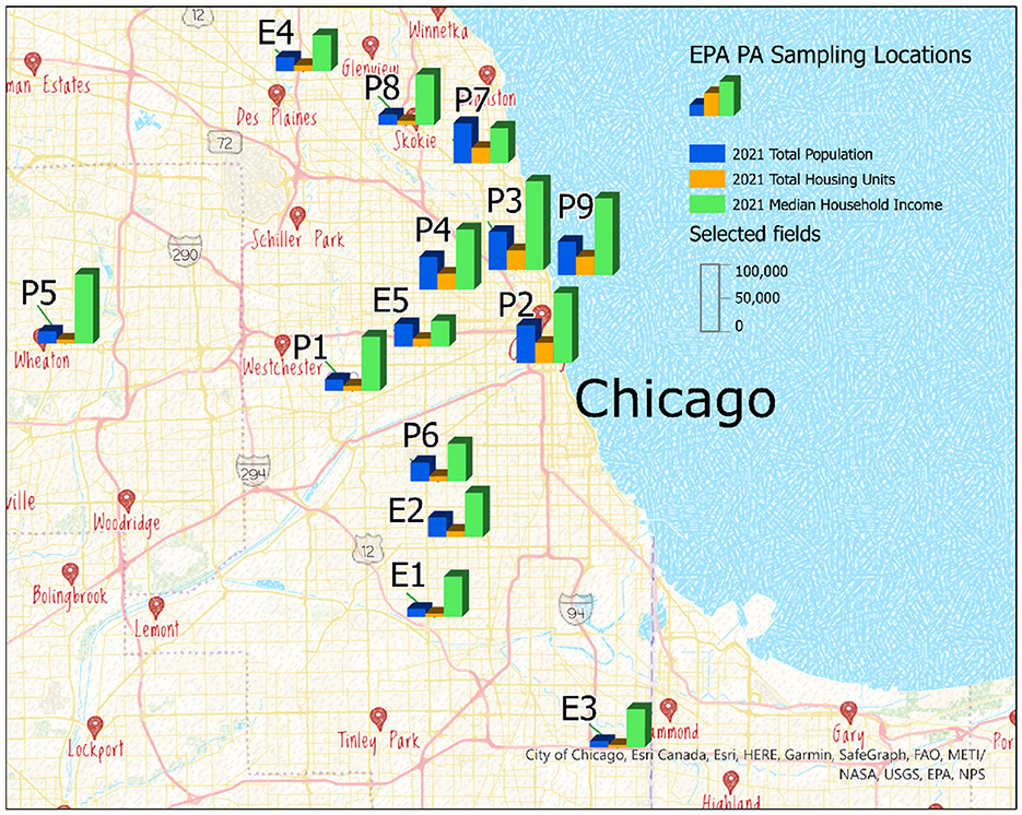
Figure 1. EPA and PurpleAir sampling locations with total population, total housing units, and median household income in Cook County IL.

2.2 Correlation analysis

The Pearson correlation coefficient was calculated to quantify the linear association between pairs of EPA, PA, and NOAA sensors using

$\begin{array}{ll}r=\frac{\sum (x_i-\bar{x})(y_i-ȳ)}{\sqrt{\sum {(x_i-\bar{x})}^2\sum {(y_i-ȳ)}^2}}& (1)\end{array}$

where x_i and y_i are the individual sample points, and $\bar{x}$ and ȳ are the means of the variables x and y, respectively. In the context of PM_2.5 measurements and meteorological data, x_i and y_i represent data from either PM_2.5 or meteorological variables.

2.3 Measurement error

To assess the significance of measurement errors between EPA and PA, we conducted Bland–Altman analysis [21]. Additionally, we performed Levene's test of equality of variances to determine whether the variability on the observed data from both EPA and PA sensors was statistically different [22].

2.4 Kolmogorov-Zurbenko (KZ) filter

Recognizing that the correction models using only RH and temperature do not uniformly account for the contribution of all sources to the PA data, particularly at the short-term component of PM_2.5 [14], we plan to investigate the source components impacting both short-term and baseline components of PM_2.5. To further examine this, we have separated the data into short-term and baseline components. The short-term component includes high-frequency data that is influenced by local anthropogenic sources such as traffic and short-term weather events. The baseline component, on the other hand, includes low-frequency data that are related to seasonal changes in weather, and changes in emission rates over time [23–25]. We ignored the medium-term component of both EPA and PA from the analysis as the medium-term component of raw PA data matches with raw EPA data.

The PM_2.5 time series data are separated into short-term and baseline components using the Kolmogorov-Zurbenko (KZ) filter technique [14, 23]. The KZ filter is a low-pass filter produced through repeated iterations of a moving average with parameters moving window (m), and iterations (p) also known as KZ_{m, p}. For details on the KZ filter formulation for air sensor data, please refer to [14].

The baseline part of PM_2.5(t) time series denoted as PM_{2.5, B}(t) and baseline part of meteorological variables' time series M_i(t) denoted as M_Bi are obtained by

$\begin{array}{ll}P{M}_{2.5,B}(t)=K{Z}_{15,3}P{M}_{2.5}(t)& (2)\end{array}$

$\begin{array}{ll}{M}_{Bi}(t)=K{Z}_{15,3}{M}_i(t)& (3)\end{array}$

The short-term part of PM_2.5(t) time series denoted as PM_{2.5, S}(t) and short-term part of meteorological time series M_i(t) denoted as M_Si(t) are obtained by

$\begin{array}{ll}P{M}_{2.5,S}(t)=P{M}_{2.5}(t)-K{Z}_{15,3}P{M}_{2.5}(t)& (4)\end{array}$

$\begin{array}{ll}{M}_{Si}(t)=M_i(t)-K{Z}_{15,3}{M}_i(t)& (5)\end{array}$

2.5 Relative contributions (%) of temporal components

By separating the data into short-term and baseline components, we can analyze and examine how each component contributes to the overall variance of the time series data for both EPA and PA PM_2.5 [26]. The relative contributions of temporal components are obtained as follows:

$\begin{array}{ll}Relativecontribution(\%)=\frac{Var(i(t))}{Var(P{M}_{2.5}(t))}·100& (6)\end{array}$

where Var(i(t)) is variance of short-term, or baseline component, and Var(PM_2.5(t)) is variance of total PM_2.5 time series.

2.6 MLR models: PM_2.5 contributions from meteorology

The short-term and baseline components of PM_2.5 can be combined with short-term and baseline components of meteorology to quantify the effect of meteorology and relatively estimate the effect of anthropogenic activities on PM_2.5 data [27–29]. The PM_2.5 data can be approximated as short-term and baseline PM_2.5 measurements as

$\begin{array}{ll}P{M}_{2.5}(t)=P{M}_{2.5,B}(t)+P{M}_{2.5,S}(t)+ϵ(t),& (7)\end{array}$

The multiple linear regression (MLR) models for short-term and baseline components of PM_2.5 with short-term and baseline meteorology and anthropogenic activities can be written as

$\begin{array}{c}P{M}_{2.5}(t)=P{M}_{2.5,S}(t)+P{M}_{2.5,B}(t)=[a_0+{\displaystyle {\sum }_{i=1}^4}{a}_i{M}_{Si}(t)]\\ +[b_0+{\displaystyle {\sum }_{i=1}^4}{b}_i{M}_{Bi}(t)]+({ϵ}_B(t)+{ϵ}_S(t)),& (8)\end{array}$

where,

$\begin{array}{ll}P{M}_{2.5,S}(t)=[a_0+{\displaystyle \sum _{i=1}^4}{a}_i{M}_{Si}(t)]+{ϵ}_S(t),& (9)\end{array}$

$\begin{array}{ll}P{M}_{2.5,B}(t)=[b_0+{\displaystyle \sum _{i=1}^4}{b}_i{M}_{Bi}(t)]+{ϵ}_B(t).& (10)\end{array}$

M_Si(t) and M_Bi(t) are time series of the i^th meteorological variable for short-term and baseline components, respectively, and a₀, b₀, a_i, and b_i are regression model parameters to be estimated using a step-wise algorithm in MLR model. The residuals ϵ_S(t), ϵ_B(t) represent changes in PM_2.5 concentrations that cannot be attributed to meteorological variables present in the model and are mainly due to anthropological activities in the short-term and baseline components, respectively [27, 28]. To estimate the impact of meteorology and anthropogenic impact on both short-term and baseline PM_2.5(t), we built models considering PM_2.5(t) data as the response variable and meteorological data from nearby NOAA sensor as the predictor variable for each EPA sensor and PA sensor. We used the variance inflation factor (VIF) to assess the multicollinearity between the explanatory variables [30].

2.7 Relative importance of predictors (LMG)

MLR models can only quantify the overall impact of meteorology on PM_2.5 measurements of both EPA and PA networks in short-term and baseline components. However, the question of which predictor most influences the data of both networks has no trivial answer due to the presence of correlated predictors. Correlation analysis is often used to examine the relationship between two variables. However, when there are many predictors, correlation analysis is not the best method to use. Here, we use the LMG measure proposed by Lindeman, Merenda, and Gold [31] and popularized by [32] to determine the relative importance of predictors.

The LMG measure uses sequential R², but it accounts for the dependence on orderings by averaging over all possible orderings. According to [33, 34], the variance decomposition for a linear model with k predictors can be defined as

$\begin{array}{ll}P{M}_{2.5}(t)={\beta }_0+{\displaystyle \sum _{i=1}^4}{\beta }_i{M}_i(t)+ϵ(t),& (11)\end{array}$

and

$\begin{array}{ll}V(P{M}_{2.5}(t))={\displaystyle \sum _{j=1}^4}{\beta }_j^2{\nu }_j^2+2{\displaystyle \sum _{j=1}^3}{\displaystyle \sum _{k=j+1}^4}{\beta }_j{\beta }_k\sqrt{{\nu }_j{\nu }_k}{\rho }_{jk}+{\sigma }^2(t),& (12)\end{array}$

where ν_j and ν_k are variances of each predictor M_i(t), and ρ_jk is the covariance of predictor j = 1, 2, 3, 4 with k = j+1, ..., 4.The R² for a model with predictors in set S is given as

$\begin{array}{ll}{R}^2(S)=\frac{\text{Model sum of square}}{\text{Total sum of square}}& (13)\end{array}$

The additional R² adding set X to a model with the predictors in set S is given by

$\begin{array}{ll}seq{R}^2(X|S)=R^2(X\cup S)-R^2(S),& (14)\end{array}$

where S and X are disjoint sets of predictors.

$\begin{array}{ll}seq{R}^2(x_k|S_k(r))=R^2(x_k\cup S_k(r))-R^2(S_k(r)),& (15)\end{array}$

where r denotes permutations, r = 1, 2, ..., p!; $seq{R}^2(x_k|r)$ denotes the sequential sum of squares for the predictors x_k in the ordering of the predictors in the r-th permutation.

The LMG measure for the k-th predictor x_k based on sequential sums of squares from all possible (p!) orderings for p predictors is given by

$\begin{array}{ll}LMG(x_k)=\frac{1}{p!}{\displaystyle \sum _{r=1}^{p!}}(seq{R}^2(x_k|r))& (16)\end{array}$

For example, for three explanatory variables (p=4), there are 24 different orderings (4!) and six different estimations (sequential sum of squares) for each explanatory variable. The relative importance of each explanatory variable is the mean of the six estimations. We applied the LMG measure, defined in Equation 16 on short-term and baseline components of PM_2.5 in Equation 9 and Equation 10 to get the relative contribution of each meteorological predictor on short-term and baseline PM_2.5, respectively.

2.8 Steps to apply this method

Step 1:

Apply the KZ filter (Equation 2 to Equation 5) to decompose the data into short-term and baseline components of the time series.

Step 2:

Quantify the relative importance (Equation 6) of short-term and baseline components; i.e., the variance of each component out of the total variance of the time series.

Step 3:

Use the LMG method (Equation 16) to quantify the impact of each correlated predictor on the short-term and baseline components of the time series.

2.9 Software

For the entire workflow (reading and organizing data, descriptive analysis, and data analyses), we used the R software (R: A Language and Environment for Statistical Computing) (version 4.2.3), along with the following libraries in our coding: readxl, dplyr, tidyr, ggplot2, car, qqplotr, kza, stats, relaimpo. The “relaimpo” package was developed by [35], which can calculate the relative importance of predictor variables in multiple regression using the LMG measure and bootstrap confidence intervals.

3 Results

3.1 Data summary and correlation analysis

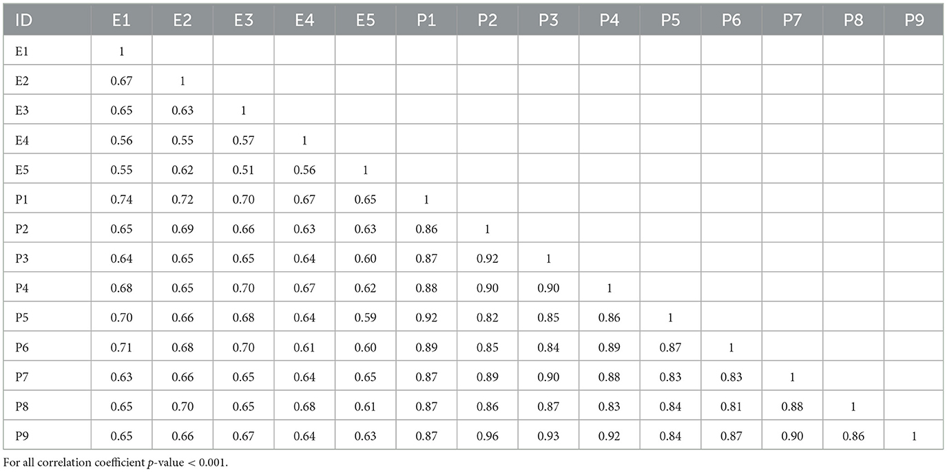
This analysis utilizes PM_2.5 time series data from 5 EPA, 9 PA sensors, and 5 NOAA monitors located in Cook County, IL, from October 2019 to September 2021. The distribution of PM_2.5 data at each of the EPA and PA sensors over the entire analysis period is presented in Table 1. The overall distribution of PA sensors is broader compared to EPA monitors with higher mean PM_2.5 concentrations. Furthermore, to understand the overall linear relationship of EPA with PA, we applied the Pearson correlation Equation 1 to each pair of EPA and PA sensors. The correlation analysis was conducted for all possible combinations: PA with PA, EPA with EPA, and PA with EPA. The results of the correlation analysis are presented in Table 2. The PA sensor network shows correlations within the PA network with correlation coefficients ranging from 0.81 to 0.90 and with EPA coefficients ranging from 0.59 to 0.72. The correlation coefficient within the EPA network ranges from 0.51 to 0.67. We calculated the correlation coefficient of meteorological variables, as shown in Supplementary Table 2. Relative humidity (RH), temperature, wind speed (WS), and wind direction (WD) are all correlated with each other. Specifically, T and RH are negatively correlated, and WS is also negatively correlated with RH and T.

Table 1

Table 1. Descriptive statistics of PM_2.5 data from EPA and PA sensors.

Table 2

Table 2. Correlation matrix of PM_2.5 data from EPA and PA sensors.

3.2 Measurement error

To assess the significance of measurement errors between EPA and PA, we conducted Bland–Altman analysis as shown in Supplementary Figure 1. The Bland–Altman analysis on EPA E2 and PA P6, the closest and comparable sensors pair, shows that measurements of E2 tend to report values that are lower than those reported by P6 and have significant measurement error. This is also reported in many earlier studies that PA sensors overestimate the measurements [12, 14]. Additionally, we applied Levene's test of equality of variances to assess whether the variances of the data from the EPA and PA sensors were statistically different. The results showed a p < 0.001 and an F-test value of 225.43. This indicates that the measurement variances from the EPA (E2) and PA (P6) sensors differ significantly. The difference in variances suggests that the measurements are inconsistent between the two sensor types.

3.3 Kolmogorov-Zurbenko (KZ) filter

To investigate the source components influencing the short-term and baseline fluctuations of low-cost sensor PM_2.5 data and to compare it with PM_2.5 data from reference monitors of EPA, we use the KZ filtering approach to separate the short-term and baseline components of the PM_2.5 time series at each selected EPA monitor and PA sensor, as well as meteorological variables including RH, temperature, WS, and WD from a nearby NOAA station, following Equations 2–5. The summary of KZ filtered short-term as baseline components is presented in Tables 3, 4. For illustration of temporal variations, one combination of EPA and PA datasets (E2 and nearby PA sensor P6), the short-term and baseline components are shown in Figure 2. The total PM_2.5 time series in Figure 2A for EPA sensor E2 has a range from 0 to 30μg/m³, whereas raw data from PA sensor P6 have an almost double range from 0 to 60μg/m³, which is also observed in the standard deviation of PA sensor data compared to EPA. Similarly, after decomposing PM_2.5 time series into short-term components as shown in Figure 2B and Table 3, the standard deviation is double in PA data compared to EPA. In the baseline component of PM_2.5 in Figure 2C, Table 4, the standard deviations in both datasets are similar, suggesting that the data have more variation in the short-term for PA sensors compared to EPA.

Table 3

Table 3. Descriptive statistics of short-term of PM_2.5 data from EPA and PA sensors.

Table 4

Table 4. Descriptive statistics of baseline of PM_2.5 data from EPA and PA sensors.

Figure 2

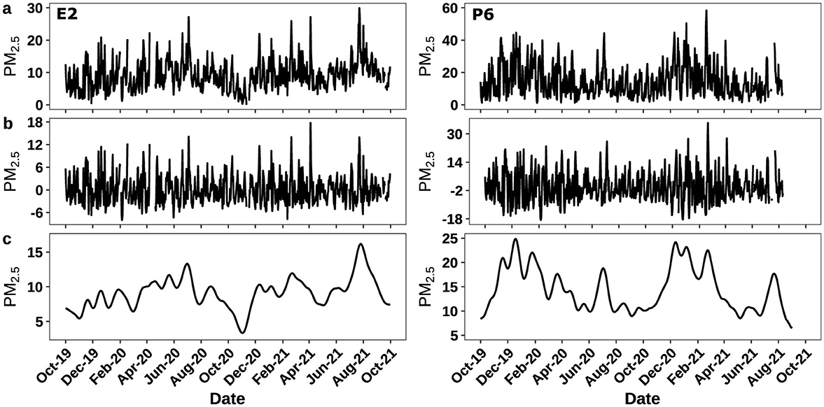
Figure 2. (a) PM_2.5 time series data from EPA sensor E2, and PA sensor P6. (b) KZ filtered short-term component for the two datasets. (c) KZ filtered baseline component for the two datasets.

3.4 Relative contributions (%) of temporal components

Our analysis of the time series decomposition revealed differences in the short-term and baseline components in both networks. By measuring the variation in each temporal component, we quantified the proportion of variation in each component relative to the total variation of the EPA and PA PM_2.5 time series data using Equation 6. The results of the relative contributions of short-term and baseline components to total data are presented in Figure 3A, Supplementary Table S3A. In Figure 3A, it can be observed that both PA and EPA PM_2.5 data have a greater relative contribution in the short-term component to the total variance, which is approximately 60–86%. However, comparing the two networks, the PA sensors have a relatively higher contribution than EPA to short-term variations. The relative contribution of the short-term component to total variance is greater in PA data, with a narrow distribution, indicating that the short-term component variance is largely uniform in the PA network and may be due to the capture of a local source that is independent of the sensor's location, as observed in correlations within the PA network in Table 2. On the other hand, the EPA sensors exhibit a broader variation in their short-term component, indicating that they capture local sources based on their location. The relative contribution of baseline to total variance is approximately 8–37%, but when comparing the two networks, the relative contribution of EPA sensors is more than that of PA sensors in the baseline component. The higher relative contribution of EPA to the baseline could be due to the impacts of meteorology as meteorology contributes to baseline trends of air quality data.

Figure 3

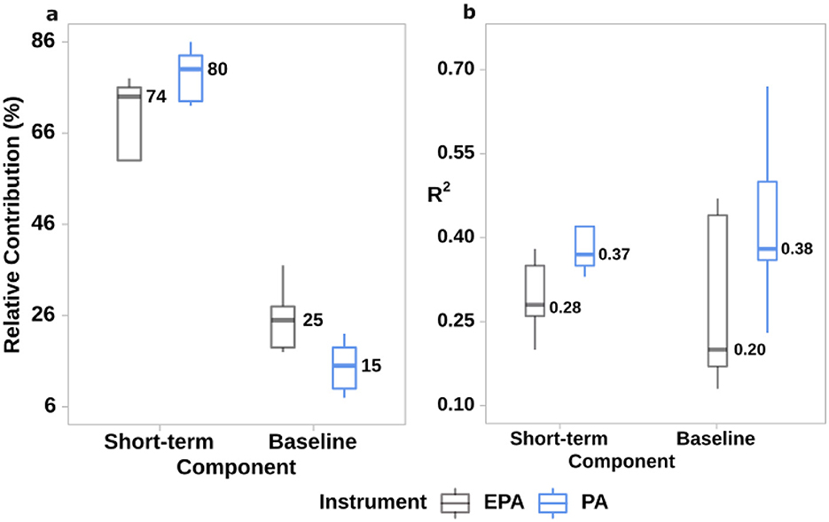
Figure 3. (a) Relative contributions of PM_2.5 (b) R² of MLR models of PM_2.5 with meteorology, both (a, b) in short-term and baseline components of EPA and PA.

3.5 MLR models: PM_2.5 contributions from meteorology

To understand and quantify the effect of meteorological conditions on the PM_2.5 data from PA and to compare with the data from EPA, we used MLR models with the stepwise forward selection algorithm. We included short-term and baseline temperature, RH, WS, and WD as meteorological predictors and short-term and baseline PM_2.5 data as response variables in our analysis. In the final model, only variables that were significant according to the stepwise forward selection algorithm were included. This technique involves adding variables one at a time based on their p-value and determines the optimal set of parameters for the model. The model performance was compared using the R² values. From the previous section, we noted that the relative contributions of short-term components were higher in PA sensors as shown in Figure 3A but looking at MLR models, meteorology has a greater impact on PA sensors' short-term variations as observed in Figure 3B. This implies that higher variations were indeed due to weather in the short-term component of low-cost PA sensors.

In Figure 3B, it can be observed that the short-term component of the PA sensors has R² ranging from 0.33 to 0.42. On average, this is 11% more R² than EPA sensors, as seen in Supplementary Table S3A. Likewise, the baseline component of PA sensors in Figure 3B, Supplementary S3A has higher R² ranging from 0.23 to 0.67. Despite having lesser relative contributions in the baseline component, it still has an average of 18% more R² than EPA sensors. This shows that weather is a higher contributor to the variance of PM_2.5 in both short-term and baseline components in low-cost sensors compared to reference monitors. The short-term and baseline components of all PA sensor PM_2.5 data have higher R² with meteorological parameters, indicating that weather influences PA sensors but is less responsive to anthropogenic emissions from traffic and other sources compared to EPA reference monitors.

We also used the variance inflation factor (VIF) to assess multicollinearity among the explanatory variables, as a complement to the LMG method. The VIF analysis indicates that when the model is fitted to the PM_2.5 time series without separating it into short-term and baseline components, all weather variables, including temperature, relative humidity (RH), wind speed (WS), and wind direction (WD), have VIF values below 2. However, after applying the KZ filter, the baseline component models show VIF values of T greater than 4 and WS greater than 2, while RH and WD remain below 2. In contrast, the short-term component has VIF values below 2 for all weather variables, suggesting that multicollinearity is present in the baseline component.

3.6 Relative importance of predictors (LMG)

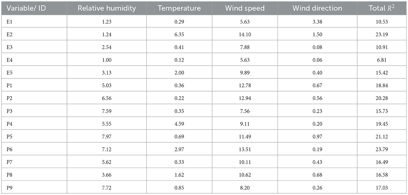
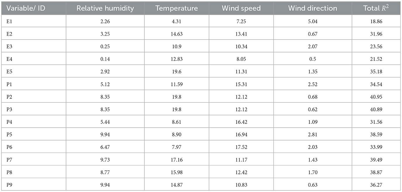
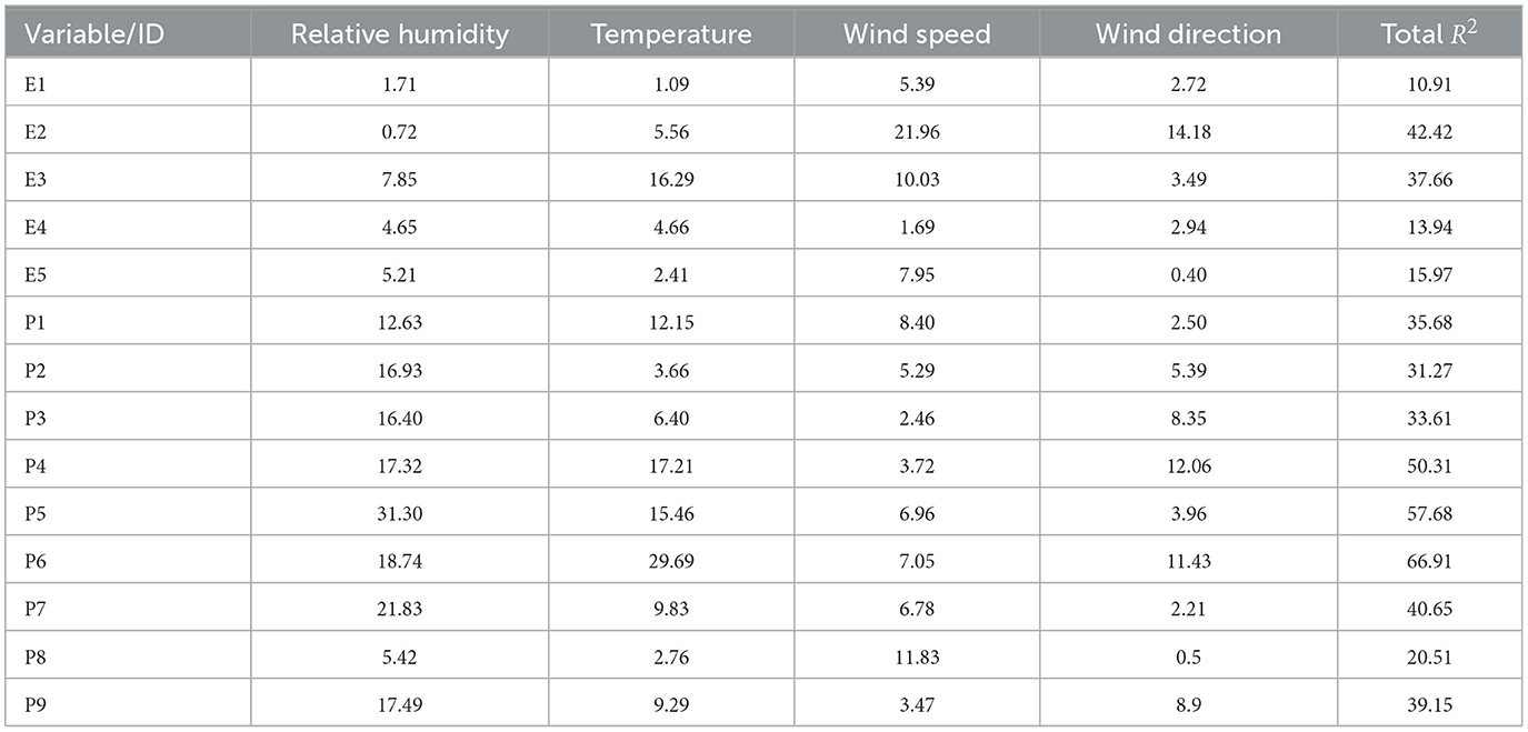
We utilized multiple linear regression models to determine that low-cost sensors are more sensitive to weather parameters compared to reference monitors, in both the short-term and baseline components. However, it is not possible to determine the individual influence of each meteorological predictor using MLR analysis due to their correlation with each other. Therefore, we used the LMG measure to determine the relative importance of each predictor in both short-term and baseline PM_2.5. The output of LMG(x_k) is partial R² for the variable that adds up to 1 for all predictors x_k, for k = 1, 2, ...., n. For our study case, k = 1, 2, 3, 4, for RH, temperature, WS, and WD. The LMG(x_k) measure was calculated using Equation 16, applied on short-term (Equation 9) and baseline (Equation 10) PM_2.5, and the results of LMG(x_k) measure for PM_2.5 time series, short-term, and baseline components of PM_2.5 are summarized and presented in Tables 5–7, Figures 4A, 4B, respectively. Based on the LMG measure, we found that wind speed (WS) is the most influential factor for both PA and EPA time series before the data are broken down into short-term and baseline components. However, if we exclude WS, relative humidity (RH) becomes the most influential factor. Once the time series is broken down into components, WS emerges as the most influential factor in almost half of the PA sensors (P1, P4, P5, and P6) in the short-term components, while the temperature is the most important factor in the short-term component of all EPA sensors except E1. In the baseline, RH consistently remains an important factor for PA sensors, except for P6 and P8. There are varying responses of meteorological factors in the baseline and short-term of both datasets.

Table 5

Table 5. Relative importance, LMG (R²) of predictors in PM_2.5 time series.

Table 6

Table 6. Relative importance, LMG (R²) of predictors in the short-term component of PM_2.5.

Table 7

Table 7. Relative importance, LMG (R²) of predictors in the baseline component of PM_2.5.

Figure 4

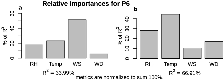
Figure 4. Relative importance (LMG) of individual meteorological variables for PA sensor P6 in (a) short-term and (b) baseline components of PM_2.5 data.

4 Discussion

Our study introduces a mathematical methodology for analyzing sensor data with high spatiotemporal resolution. We analyzed 2 years of PM_2.5 monitoring data from EPA reference monitors and PA low-cost air sensors. Comparing raw PA PM_2.5 data to EPA monitors' PM_2.5 data, it is evident that the EPA monitors' data are consistently lower than the EPA standard limit of PM_2.5 set by the EPA (9 μg/m³. However, the mean values from raw PA sensors exceed this recommended standard limit. This is because PA data tend to overestimate PM_2.5 and require calibration use in health analysis and policy decisions.

Correlation analysis showed that within the PA network correlations were higher than those within the EPA network, regardless of sensors locations. Moreover, the PA sensors exhibit strong correlations with EPA sensors across various locations. It should be noted that the high observations in the PA network may be adjusted after calibrating the PA data using weather parameters such as relative humidity (RH) and temperature, as discussed in a previous study [12, 14]. However, the correction models built using RH and temperature can adjust the baseline, but the short-term component becomes underestimated after corrections. Short-term changes in air quality data are typically due to local temporal sources such as traffic and short-term weather variations, as described by [23–25].

Our study also examined the impact of WS and WD on short-term PA PM_2.5 levels, a topic that has not been thoroughly investigated, with only a few studies, including [15], addressing this issue. It has not been investigated which meteorological variable contributes more to the variability in PA data, both in short-term and baseline components, compared to the EPA. This comparison is important due to the correlated nature of meteorological variables.

We also calculated the relative contribution of short-term and baseline components of PM_2.5 out of the time series of PM_2.5. The PA sensors located in urban areas near the lake, specifically P2, P3, P7, P8, and P9, have a higher relative contribution in the short-term component compared to other PA sensors. This increased contribution of low-cost sensors to the total variance at most locations, particularly in highly populated areas near the lake, can be attributed to weather patterns. It is worth noting that this pattern was not observed by [14] in the power spectral density (PSD) analysis of high-frequency signals (4, 8, 12, and 24 h) in short-term, which are primarily related to anthropogenic activities. It has also been observed that the performance of low-cost sensors in capturing particle size and optical properties can be influenced by weather conditions at certain locations, leading to higher variations in data readings.

We further quantify the impact of meteorological parameters using linear regression models in both short-term and baseline components. The PA sensor PM_2.5 has higher R² values in both short-term and baseline components. However, with linear regression models, it is not clear which meteorological variable is impacting the data, as all variables, specifically temperature, RH, WS, and WD, are correlated. The third step in our method is to apply the LMG method on KZ-filtered short-term and baseline PM_2.5. According to the LMG measure, WS is the most influential factor for both PA and EPA time series before the decomposition of the data into short-term and baseline components. Additionally, if we remove WS, RH becomes the most influential factor, as found by earlier studies [12]. However, after decomposing the time series into components, WS is the most influential factor in most of the PA sensors in the short-term components, whereas temperature is the most important factor in the short-term component of most EPA sensors. In the baseline, RH is a consistently important factor for PA sensors aligning with findings of earlier studies [12].

It is worth noting that meteorological factors have varying effects on both networks. RH is the only useful factor for baseline (low-frequency) components but not for short-term (high-frequency) components. However, previous studies by [12, 13, 36] have used only RH for PA corrections in both components, i.e., the time series of PM_2.5, even though sensor performance depends on the location. The reason for the impact of wind speed on the PA sensor may be due to its inlet orientation being at a 90° angle to the wind, which causes upward flow and the low inlet velocity through the sampling holes can result in significant losses of larger particles [15, 37].

This study has a few limitations. One of them is the limited number of co-located sensors, which are important for comparing responses from both reference monitors and low-cost sensors. Another limitation is the assumption of linearity in the data and keeping the range of PM_2.5 data from 0 to 70 μg/m³. This was done to ensure a fair comparison to standard approaches for air sensor data corrections. However, this method might not work beyond this data range due to non-linearity in the data. The next step could be testing this method on a wider range of sensor data across the US and also without restricting the PM_2.5 data range.

5 Conclusion

In this study, we propose a mathematical technique to analyze air sensor data, specifically identifying the key correlated environmental factors impacting the data across different temporal components. These components include short-term changes driven by anthropogenic activities and weather variations, as well as baseline changes resulting from seasonal shifts in weather and meteorology. By employing time series decomposition using the Kolmogorov–Zurbenko (KZ) filter and assessing each predictor's impact with the Lindeman, Merenda, and Gold (LMG) method, we effectively analyzed PM_2.5 data from both EPA and PA networks. This analysis suggests that PA sensors are more sensitive to meteorological conditions, particularly wind speed in the short-term and relative humidity (RH) in the baseline components. Previous studies have typically only considered RH for correction models. Our technique provides a valuable tool for analyzing air sensor data and developing robust, location-specific calibration strategies. Future research could extend this method to additional sensors in various geographical locations as more air sensors are deployed globally.

Data availability statement

Publicly available datasets were analyzed in this study. This data can be found here: https://aqs.epa.gov/aqsweb/documents/data_api.html; https://community.purpleair.com/t/purpleair-data-download-tool/3787p604800/cC0#11.44/41.8363/-87.6973; https://www.ncei.noaa.gov/products/climate-data-records.

Author contributions

VK: Conceptualization, Methodology, Data Curation, Visualization, Investigation, Formal analysis, Writing – original draft. SS: Conceptualization, Methodology, Supervision, Validation, Writing – review & editing. DS: Data curation, Writing – review & editing. SG: Conceptualization, Validation, Supervision, Writing – review & editing. SD: Conceptualization, Methodology, Supervision, Validation, Writing – review & editing. SM: Conceptualization, Project administration, Supervision, Validation, Writing – review & editing.

Funding

The author(s) declare that no financial support was received for the research, authorship, and/or publication of this article.

Acknowledgments

Vijay Kumar acknowledges the support from the US-Pakistan Knowledge Corridor Ph.D. Scholarship Program under the Higher Education Commission, Pakistan.

Conflict of interest

The authors declare that the research was conducted in the absence of any commercial or financial relationships that could be construed as a potential conflict of interest.

The author(s) declared that they were an editorial board member of Frontiers, at the time of submission. This had no impact on the peer review process and the final decision.

Publisher's note

All claims expressed in this article are solely those of the authors and do not necessarily represent those of their affiliated organizations, or those of the publisher, the editors and the reviewers. Any product that may be evaluated in this article, or claim that may be made by its manufacturer, is not guaranteed or endorsed by the publisher.

Supplementary material

The Supplementary Material for this article can be found online at: https://www.frontiersin.org/articles/10.3389/fams.2024.1368147/full#supplementary-material

References

1. Li L, Losser T, Yorke C, Piltner R. Fast inverse distance weighting-based spatiotemporal interpolation: a web-based application of interpolating daily fine particulate matter PM2.5 in the contiguous US using parallel programming and KD tree. Int J Environm Res Public Health. (2014) 11:9101–41. doi: 10.3390/ijerph110909101

PubMed Abstract | Crossref Full Text | Google Scholar

2. Wang Q, Liu S. The effects and pathogenesis of PM2. 5 and its components on chronic obstructive pulmonary disease. Int J Chronic Obstruct Pulmon Dis. (2023) 18:493–506. doi: 10.2147/COPD.S402122

PubMed Abstract | Crossref Full Text | Google Scholar

3. Raaschou-Nielsen O, Andersen ZJ, Beelen R, Samoli E, Stafoggia M, Weinmayr G, et al. Air pollution and lung cancer incidence in 17 European cohorts: prospective analyses from the European Study of Cohorts for Air Pollution Effects (ESCAPE). Lancet Oncol. (2013) 14:813–22. doi: 10.1016/S1470-2045(13)70279-1

PubMed Abstract | Crossref Full Text | Google Scholar

4. Wu X, Nethery RC, Sabath MB, Braun D, Dominici F. Exposure to air pollution and COVID-19 mortality in the United States: a nationwide cross-sectional study. medRxiv. (2020). doi: 10.1101/2020.04.05.20054502

PubMed Abstract | Crossref Full Text | Google Scholar

5. Zhou X, Josey K, Kamareddine L, Caine MC, Liu T, Mickley LJ, et al. Excess of COVID-19 cases and deaths due to fine particulate matter exposure during the 2020 wildfires in the United States. Sci Adv. (2021) 7:eabi8789. doi: 10.1126/sciadv.abi8789

PubMed Abstract | Crossref Full Text | Google Scholar

6. Mondal S, Chaipitakporn C, Kumar V, Wangler B, Gurajala S, Dhaniyala S, et al. COVID-19 in New York state: effects of demographics and air quality on infection and fatality. Sci Total Environm. (2022) 807:150536. doi: 10.1016/j.scitotenv.2021.150536

PubMed Abstract | Crossref Full Text | Google Scholar

7. Chaipitakporn C, Athavale P, Kumar V, Sathiyakumar T, Budisic M, Sur S, et al. COVID-19 in the United States during pre-vaccination period: shifting impact of sociodemographic factors and air pollution. Front Epidemiol. (2022) 2:48. doi: 10.3389/fepid.2022.927189

PubMed Abstract | Crossref Full Text | Google Scholar

8. Kioumourtzoglou MA, Spiegelman D, Szpiro AA, Sheppard L, Kaufman JD, Yanosky JD, et al. Exposure measurement error in PM 2.5 health effects studies: a pooled analysis of eight personal exposure validation studies. Environm Health. (2014) 13:1–11. doi: 10.1186/1476-069X-13-2

PubMed Abstract | Crossref Full Text | Google Scholar

9. Dominici F, Zanobetti A, Schwartz J, Braun D, Sabath B, Wu X. Assessing adverse health effects of long-term exposure to low levels of ambient air pollution: implementation of causal inference methods. Res Rep Health Eff Inst. (2022) 2022:1–56.

PubMed Abstract | Google Scholar

10. PurpleAir. Purple Air: Public Database of Sensors Installed in Entire World. (2024). Available at: https://map.purpleair.com/1/mAQI/a (accessed January 03, 2024).

Google Scholar

11. PurpleAir. PurpleAir.: PublicLab. (2020). Available at: https://publiclab.org/wiki/purpleair (accessed June 05, 2023).

Google Scholar

12. Barkjohn KK, Gantt B, Clements AL. Development and application of a United States-wide correction for PM 2.5 data collected with the PurpleAir sensor. Atmospheric Measurem Techniq. (2021) 14:4617–37. doi: 10.5194/amt-14-4617-2021

PubMed Abstract | Crossref Full Text | Google Scholar

13. Ardon-Dryer K, Dryer Y, Williams JN, Moghimi N. Measurements of PM 2.5 with PurpleAir under atmospheric conditions. Atmosph Measur Techniq. (2020) 13:5441–58. doi: 10.5194/amt-13-5441-2020

Crossref Full Text | Google Scholar

14. Kumar V, Senarathna D, Gurajala S, Olsen W, Sur S, Mondal S, et al. Spectral analysis approach for assessing accuracy of a low-cost air quality sensor network data. Atmosph Measur Techniq. (2023) 2023:1–20. doi: 10.5194/amt-2023-62

Crossref Full Text | Google Scholar

15. Ouimette JR, Malm WC, Schichtel BA, Sheridan PJ, Andrews E, Ogren JA, et al. Evaluating the PurpleAir monitor as an aerosol light scattering instrument. Atmosph Measur Techniq. (2022) 15:655–76. doi: 10.5194/amt-15-655-2022

Crossref Full Text | Google Scholar

16. Owusu-Tawiah V, Westervelt DM, Annor T. Relationships Between Meteorological Parameters and PM2. 5 in Accra. In: International Conference on Air Quality in Africa. Cham: Springer (2022). p. 81–83.

Google Scholar

17. Molina Rueda E, Carter E. L'Orange C, Quinn C, Volckens J. Size-resolved field performance of low-cost sensors for particulate matter air pollution. Environm Sci Technol Letters. (2023) 10:247–53. doi: 10.1021/acs.estlett.3c00030

PubMed Abstract | Crossref Full Text | Google Scholar

18. Ouimette J, Arnott WP, Laven P, Whitwell R, Radhakrishnan N, Dhaniyala S, et al. Fundamentals of low-cost aerosol sensor design and operation. Aerosol Sci Technol. (2024) 58:1–15. doi: 10.1080/02786826.2023.2285935

PubMed Abstract | Crossref Full Text | Google Scholar

19. EPA. US Environmental Protection Agency (EPA): Publically Available Air Quality Data API. (2024). Available at: https://aqs.epa.gov/aqsweb/documents/data_api.html (accessed January 03, 2024).

Google Scholar

20. NOAA. National Oceanic and Atmospheric Administration (NOAA): Public Database (2024). Available at: https://www.ncei.noaa.gov/products/climate-data-records (accessed January 03, 2024).

Google Scholar

21. Karun KM, Puranik ABA. plot: an R function for Bland-Altman analysis. Clini Epidemiol Global Health. (2021) 12:100831. doi: 10.1016/j.cegh.2021.100831

Crossref Full Text | Google Scholar

22. Gastwirth JL, Gel YR, Miao W. The impact of Levene's test of equality of variances on statistical theory and practice. Statist Sci. (2009) 24:343–60. doi: 10.1214/09-STS301

Crossref Full Text | Google Scholar

23. Rao ST, Zurbenko IG. Detecting and tracking changes in ozone air quality. Air Waste. (1994) 44:1089–92. doi: 10.1080/10473289.1994.10467303

PubMed Abstract | Crossref Full Text | Google Scholar

24. Rao S, Zurbenko I, Neagu R, Porter P, Ku J, Henry R. Space and time scales in ambient ozone data. Bull Am Meteorol Soc. (1997) 78:2153–66.

Google Scholar

25. Wise EK, Comrie AC. Meteorologically adjusted urban air quality trends in the Southwestern United States. Atmos Environ. (2005) 39:2969–80. doi: 10.1016/j.atmosenv.2005.01.024

Crossref Full Text | Google Scholar

26. Botlaguduru VS, Kommalapati RR, Huque Z. Long-term meteorologically independent trend analysis of ozone air quality at an urban site in the greater Houston area. J Air Waste Managem Assoc. (2018) 68:1051–64. doi: 10.1080/10962247.2018.1466740

PubMed Abstract | Crossref Full Text | Google Scholar

27. Bai H, Gao W, Zhang Y, Wang L. Assessment of health benefit of PM2.5 reduction during COVID-19 lockdown in China and separating contributions from anthropogenic emissions and meteorology. J Environm Sci. (2022) 115:422–31. doi: 10.1016/j.jes.2021.01.022

PubMed Abstract | Crossref Full Text | Google Scholar

28. Li K, Jacob DJ, Liao H, Shen L, Zhang Q, Bates KH. Anthropogenic drivers of 2013-2017 trends in summer surface ozone in China. Proc Nat Acad Sci. (2019) 116:422–7. doi: 10.1073/pnas.1812168116

PubMed Abstract | Crossref Full Text | Google Scholar

29. Zhai S, Jacob DJ, Wang X, Shen L, Li K, Zhang Y, et al. Fine particulate matter (PM 2.5) trends in China, 2013-2018: separating contributions from anthropogenic emissions and meteorology. Atmosph Chem Phys. (2019) 19:11031–41. doi: 10.5194/acp-19-11031-2019

Crossref Full Text | Google Scholar

30. Kutner MH, Nachtsheim CJ, Neter J, Li W. Applied Linear Statistical Models. New York: McGraw-Hill. (2005).

Google Scholar

31. Lindeman RH, Merenda PF, Gold RZ. Introduction to Bivariate and Multivariate Analysis (Vol. 4). Glenview, IL: Scott; Foresman (1980).

Google Scholar

32. Kruskal W. Relative importance by averaging over orderings. Am Stat. (1987) 41:6–10. doi: 10.1080/00031305.1987.10475432

Crossref Full Text | Google Scholar

33. Bi J, A. review of statistical methods for determination of relative importance of correlated predictors and identification of drivers of consumer liking. J Sens Stud. (2012) 27:87–101. doi: 10.1111/j.1745-459X.2012.00370.x

Crossref Full Text | Google Scholar

34. Grömping U. Variable importance in regression models. Wiley Interdisc Rev: Comp Stat. (2015) 7:137–52. doi: 10.1002/wics.1346

Crossref Full Text | Google Scholar

35. Grömping U. Relative importance for linear regression in R: the package relaimpo. J Statist Softw. (2007) 17:1–27. doi: 10.18637/jss.v017.i01

PubMed Abstract | Crossref Full Text | Google Scholar

36. Mei H, Han P, Wang Y, Zeng N, Liu D, Cai Q, et al. Field evaluation of low-cost particulate matter sensors in Beijing. Sensors. (2020) 20:4381. doi: 10.3390/s20164381

PubMed Abstract | Crossref Full Text | Google Scholar

37. Hangal S, Willeke K. Overall efficiency of tubular inlets sampling at 0-90 degrees from horizontal aerosol flows. Atmosph Environm Part A Gen Topics. (1990) 24:2379–86. doi: 10.1016/0960-1686(90)90330-P

Crossref Full Text | Google Scholar

38. Bureau UC. US Census Bureau: Public Database (2021). Available at: https://www.census.gov/geo/maps-data/data/tallies/tractblock.html (accessed April 28, 2023).

Google Scholar