 Prizka Rismawati Arum
 Ihsan Fathoni Amri2
- 1Department of Statistics, Faculty of Science and Agriculture Technology, Universitas Muhammadiyah Semarang, Semarang, Indonesia
- 2Department of Data Sciences, Faculty of Science and Agriculture Technology, Universitas Muhammadiyah Semarang, Semarang, Indonesia
Economic growth is essential for regional economic performance, with gross regional domestic product (GRDP) being a key indicator of economic development over time. In this research case, the GRDP data of various provinces on Java Island from 2010 to 2023 will be used as the variable being studied. The data obtained from the GRDP variable contain spatial and temporal information, requiring an appropriate model to forecast spatiotemporal data, namely, the Generalized Space–Time Autoregressive (GSTAR) model. However, in estimating the parameters, the GSTAR model is unable to detect correlated residuals between equations, resulting in inefficient estimators. Therefore, an appropriate estimation method is needed to address correlated residuals within the seemingly unrelated regression (SUR) framework, namely, the Generalized Least Square (GLS) estimation method. The GSTAR-SUR method is applied to forecast the economic growth rate of Java Island. The optimal model, GSTAR-SUR (11)-I(1) with inverse distance location weights, demonstrates high accuracy with a mean absolute percentage error (MAPE) of 8.451%. Forecasts for Banten, DKI Jakarta, West Java, Central Java, East Java, and DI Yogyakarta predict consistent monthly GRDP increases through December 2024.
1 Introduction
Economic development takes center stage in the development of many developing nations, including Indonesia. The aim of economic development is to stimulate various renewals in other aspects of life (1). Siagian (2) points out that the field of economics, especially in economic development, is a primary focus faced by developing countries. According to Badan Pusat Statistika (BPS) (3), the Central Statistics Agency, economic development is an effort with the goal of improving the living standards of the population. Success in the economic sector benefits the welfare of society. Therefore, economic growth is crucial in evaluating the economic performance of a region. One of the indicators used to assess the level of economic development in a specific period is the gross regional domestic product (GRDP).
Java Island is the island with the highest average GRDP in Indonesia. It comprises six provinces, namely, Banten, DKI Jakarta, West Java, Central Java, East Java, and DI Yogyakarta. This research focuses on these six provinces because they contribute significantly to the GRDP of Java Island, making its GRDP the highest among all the islands in economic development. The GRDP data fall under time series data, which can be analyzed using time series analysis methods. Time series consists of a sequence of observational data from a fixed source occurring at consecutive time indices with a constant time interval (4). The time series analysis can be used to forecast data for several future periods, making it invaluable for planning the times to come. Given the multitude of variables under examination, time series data can be categorized into two types, namely, univariate time series and multivariate time series. Univariate time series involves the analysis of a single variable, while multivariate time series entails the analysis of multiple variables in the research due to their presumed interdependencies (5).
The movement of the population to a specific region also plays a significant role in influencing the economic growth in that area. Consequently, there exists an interconnection between regions, known as spatial correlation, which affects the GRDP of the leading sector. The development of a model that takes into account spatial effects in the research on the leading sector of GRDP has also been undertaken by Nofitasari et al. (6) in their analysis of the industrial sector GRDP using a spatial regression approach. A model that integrates the relationships of previous events and incorporates the correlation with locations in multivariate time series data is referred to as a space–time model (7–10). In 1980, Pfeifer and Deutsch introduced a model that combines temporal and spatial interdependencies, known as the Space–Time Autoregressive (STAR) model. However, the STAR model is limited in parameter flexibility, as it assumes that locations are homogenous. Therefore, when dealing with locations that exhibit heterogeneous characteristics, the STAR model is less suitable to use (7, 10, 11). To address this limitation (9), the Generalized Space–Time Autoregressive (GSTAR) model was developed. The GSTAR model is an extension of the STAR model, allowing autoregressive (AR) parameter values to vary at each location and making it adaptable for use in heterogeneous locations. Research conducted by Fransiska et al. (12) on rainfall forecasting in Bengkulu province produced the GSTAR model (1.1) using uniform weight and distance inverse weight. The other research studies conducted by Huda and Imro’ah (13) regarding the GSTAR model for the COVID-19 case study on Java Island found that the weight matrix, a feature of the GSTAR model and a representation of spatial impact, plays a significant role in identifying the optimal model for further predictions.
The parameter estimation studies using GSTAR have been primarily limited to ordinary least square (OLS) estimation methods (14). As a result, GSTAR models with correlated residuals can yield less efficient estimators due to the increased likelihood of larger errors during forecasting. To address this issue, the generalized least square (GLS) method is employed to estimate parameters with correlated residuals, which is commonly used in the seemingly unrelated regression (SUR) model. The SUR model is a multivariate linear regression model introduced by Zellner, consisting of several regression equations in which the errors are uncorrelated within a single equation but are correlated across equations (15, 16). SUR research conducted by Tiong et al. (17), with a case study analysis of factors influencing train arrival delays, employed the SUR method to obtain efficient parameter estimation values for spatiotemporal data. A comparative study between GSTAR-OLS and GSTAR-SUR was conducted by Yundari and Perdana (18) in the context of applying GSTAR-SUR to the number of domestic airline passengers at Indonesian Airports. The results indicated that the GSTAR-SUR method outperformed GSTAR-OLS. In addition, Septyaningrum (19) conducted research on forecasting the number of tourists at three tourist locations in Pacitan Regency using the GSTAR-SUR method. Another research conducted by Adella et al. (20) with a case study of the number of tourists in Central Java produced the GSTAR (2.1) model, and there was a correlation between the residuals, so it was continued using the GSTAR-SUR method. The findings showed that GSTAR-SUR exhibited superior forecasting accuracy, with smaller root mean square error (RMSE) values across all tourist sites. Based on the above discussion, this research will employ the GSTAR-SUR method to analyze the GRDP in various provinces on Java Island. The goal of this study is to forecast the economic growth rate in Indonesia.
2 Methods
2.1 Search on data and research
The data used in this study consist of the GRDP of six provinces on Java Island from January 2010 to March 2023, with 318 data points sourced from BPS Java Island. The method used in this research is GSTAR-SUR. The first step involves analyzing the descriptive statistics of the data and checking stationarity. The second step is identifying the time order using the modified partial autocorrelation function (MPACF) and selecting the model order based on the minimum Akaike information criterion (AIC). Following this, spatial weights are determined for the analysis. The research steps continued by estimating the p-order parameters with the GSTAR-OLS model and carrying out residual correlation tests between locations. If there is a residual correlation between locations, the parameters of the GSTAR-SUR model are estimated using the GLS method. The next step is to test the significance of the GSTAR-SUR model parameters and carry out model feasibility tests. The final step in this research is to test the goodness of the GSTAR-SUR model based on the MAPE value and forecast the GRDP data of six provinces on Java Island (Table 1).
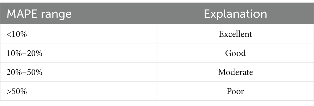
Table 1. MAPE criteria.
2.2 Multivariate time series
Multivariate time series refers to a sequence of data that consist of several variables obtained over time and recorded in chronological order at regular time intervals (16). Multivariate time series analysis is typically used for datasets that involve more than one time series, resulting in multiple variables within the model. Similar to univariate time series, the analysis of multivariate time series also takes into account the concept of data stationarity (21–23).
2.3 Generalized space–time autoregressive model
The spatial model is a framework designed to elucidate interrelationships between various geographic locations. Within datasets, it is not uncommon to encounter information that possesses not only temporal interdependencies but also spatial associations. Data exhibiting both temporal and locational dependencies can be effectively characterized using the space–time model. The space–time model serves as a formal representation of multiple observations that span both temporal and spatial dimensions, with exists at each of the N locations in a given space (i = 1, 2, …, N) with respect to the time period t. The location effects on the model are expressed as spatial weighting matrices, while the time effects are formulated as time series models. The STAR model is a classification of models that are characterized by lag, which exerts a linear influence both in terms of location and time (24). The STAR model can only be applied to homogeneous locations, based on the assumption that current research is influenced by past time within the same location.
The GSTAR model is an extension of the STAR model, with its primary distinction lying in the autoregressive parameters. In the STAR model, autoregressive parameters are assumed to be uniform, whereas, in the GSTAR model, they are presumed to be heterogeneous. Using matrix notation, the GSTAR model with autoregressive order p and spatial orders ,,…, is formulated as follows (22, 25):
Where:
= The observation vector of size (n × l) pertains to n locations at time t.
= The observation vector of size (n × l) for n locations at time (t-k).
W = The weighting matrix of size (n × n).
= diag ( = The diagonal matrix of autoregressive parameters for lag time 1.
= diag ( = The diagonal matrix of autoregressive parameters for lag time 1 and spatial lag 1.
= The residual vector normally distributed with a mean of 0 and a variance–covariance matrix .
2.4 Location weights in the GSTAR model
The selection of location weights in the GSTAR model is divided into three categories: uniform weights, inverse distance weights, and cross-correlation normalization.
2.4.1 Uniform location weights
Uniform location weights assign the same weight to every location. Ruchjana (9) defines the selection of uniform location weights as follows:
With , expressing the number of locations adjacent to location i at spatial lag 1. The weights in this model have the following properties:
The weight at lag 1 is expressed by W in the form of a matrix as stated below:
2.4.2 Inverse distance location weights
Values in the inverse distance location weights are obtained based on the actual inverse distances and then normalized. The initial matrix form is as follows:
Then, the matrix is standardized to satisfy the weight properties with the assumption that locations that are close in proximity have stronger relationships; in general, the inverse distance weight for each location is expressed as follows (13):
With the number of weights for each location being 1, and . The diagonal matrix of inverse distance weights = 0, as a location is considered to have no distance from itself; the resulting inverse distance matrix is as follows (21):
2.4.3 Cross-correlation normalization location weights
According to Setiawan et al. (16), the determination of cross-correlation weights uses cross-correlation between corresponding lag locations, with the sample estimate of cross-correlation as follows:
Where:
= The correlation value between location i and location j.
= The sample mean of the corresponding time series component i for a stationary process vector.
= The sample mean of the corresponding time series component i for a stationary process vector.
The determination of cross-location normalization weight values at corresponding time lags is assumed as follows:
Based on cross-location cross-correlation values at corresponding times, location weights with normalization allow for the presence of relationships between locations. These weights also provide flexibility in the magnitude and direction of relationships between locations whether they are positive or negative (16).
2.5 Seemingly unrelated regression model
The seemingly unrelated regression (SUR) model is a multivariate linear regression model first introduced by Zellner (15). This model consists of several regression equations, where the errors are uncorrelated within an equation but are correlated across equations. The test used to determine whether the variance–covariance error structure is indeed an SUR structure is the Lagrange multiplier test with the hypothesis (16) as follows:
H0 = for all (the variance–covariance error structure is heteroskedastic, and there is no correlation among the errors across equations).
H1 = for all (the variance–covariance error structure is heteroskedastic, and there is a correlation among the errors across equations).
The Lagrange multiplier test statistic is as follows:
With T as the number of observations, is the correlation between errors in equations i and j. With a significance level , the critical region is acquired, which is H0 rejected if .
Information regarding the correlated errors across equations can be used to improve parameter estimation in the model using GLS. GLS is an estimation method for regression parameters, which takes into account the correlation between errors across equations, where the errors are obtained from OLS estimation and later used to calculate regression coefficient estimates in the SUR model. In general, the SUR model for N observations, with each equation comprising K predictor variables, can be formulated as follows (17):
With i = 1, 2, …, N.
The SUR model has assumption as follows:
With shows the relationship of errors where:
Where:
= An identity matrix size (T)
Matrix size (M)
The error variances of each equation for i = j and the error covariance variances across equations for i.
The estimator for GLS parameters is . GLS estimators possess the properties of unbiasedness and efficiency (26, 27).
2.6 Feasibility test for the GSTAR-SUR model
Once the significant parameters and model have been obtained, it is necessary to perform a model feasibility test. The GSTAR-SUR model is considered feasible if the residuals meet the white noise assumption. White noise residuals follow an identical independent distribution and can be detected using residual autocorrelation tests in the error analysis. The white noise assumption test can be conducted using the Ljung–Box test with the following hypotheses:
H0: (residuals are not white noise).
H1: at least one , k = 1,2, …, k (residuals are white noise).
The statistics test is as follows:
Where:
n = number of data, k = number of periods tested, and = the hypothesis of residual autocorrelation at lag k as testing criteria: Rejecting the hypothesis H0 if at a significance level of (28).
2.7 Evaluation of the GSTAR-SUR model
Mean absolute percentage error (MAPE) is the average value of the absolute differences between predictions and actual values, which is expressed as a percentage of the actual value. MAPE is used to evaluate the accuracy of forecasts by calculating the error as a percentage of the actual values over a specified time period, providing information on the percentage of underestimation or overestimation. According to Khair et al. (29), the MAPE value can be calculated using the equation as follows:
With , the actual value at time t denoted as , and the forecasted value at time t denoted as n.
The MAPE value can be used when evaluating forecast results, to assess the accuracy of the predicted figures compared with the actual values. The criteria for interpreting MAPE can be as follows (30).
3 Results
3.1 Descriptive analysis
Descriptive analysis is conducted with the aim of providing a general overview of the data used in the research. The data used in this study consist of the GRDP of six provinces on Java Island from January 2010 to March 2023, with 318 data points. The description provided includes the mean, standard deviation, minimum value, and maximum value of the data.
The GRDP in Java Island is typically derived from the aggregation of six provinces on Java Island, namely, Banten, DKI Jakarta, West Java, Central Java, DI Yogyakarta, and East Java. As shown in Table 2, it can be observed that the average GRDP values vary for each of the six provinces on a monthly basis. The highest average is in East Java with a value of 299626.51, while the lowest average is in the DI Yogyakarta with a value of 9,036.8. In terms of standard deviation, the province with the greatest variability in GRDP is East Java with a value of 87667.82, and the lowest is the DI Yogyakarta with a value of 2356.49. The smallest GRDP value is 3825.83 for Banten, 84164.61 for DKI Jakarta, 162505.1 for West Java, 100535.56 for Central Java, 5014.64 for the DI Yogyakarta, and 154152.92 for East Java. The highest GRDP values are 97224.01 for Banten, 263212.22 for DKI Jakarta, 423487.62 for West Java, 266513.81 for Central Java, 14500.79 for DI Yogyakarta, and 460997.67 for East Java. The time series plot is presented in Figure 1 as follows.
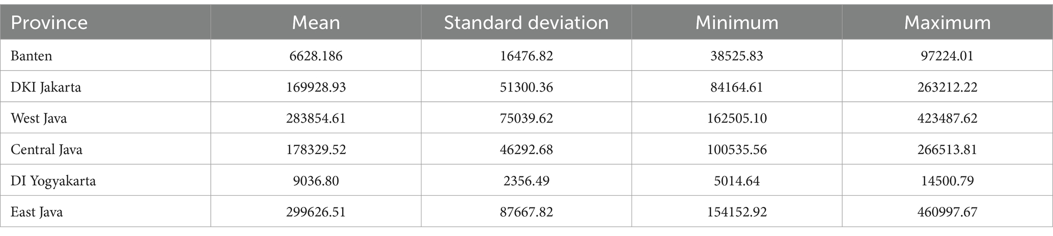
Table 2. Descriptive analysis.
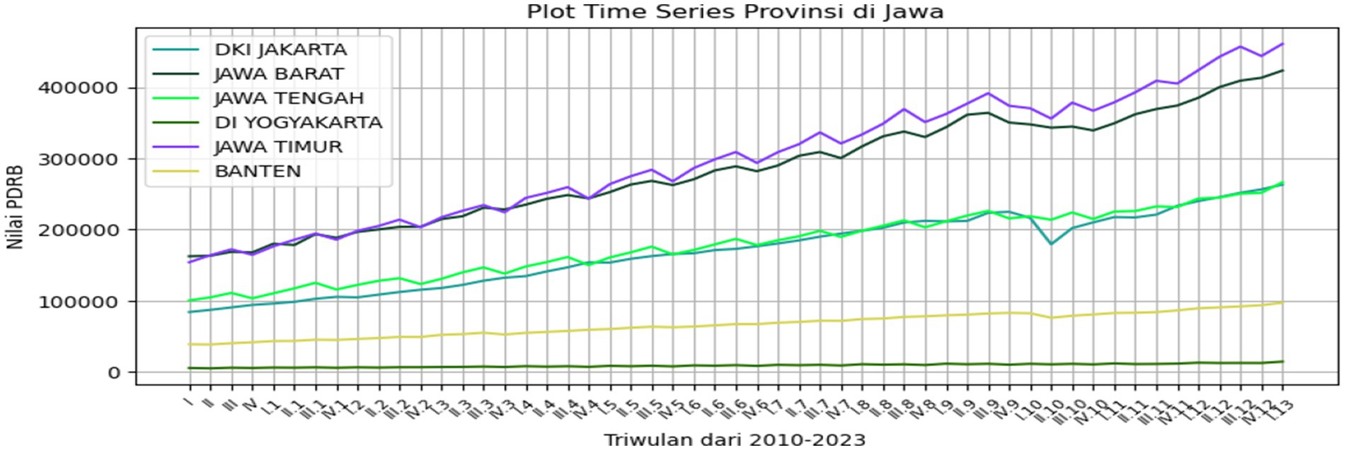
Figure 1. Plot of the GRDP in provinces.
As shown in Figure 1, it is evident that the time series plot of the GRDP does not exhibit a seasonal pattern in each plot. Looking at the time series plots, the GRDP values intersect between West Java and East Java and DKI Jakarta and Central Java, while Banten and DI Yogyakarta are the provinces with the lowest GRDP values among the six provinces.
3.2 Correlation of GDRP data for six provinces
The correlation values between regions indicate the degree of association between one region and another. The correlation values between the six provinces are presented in Table 3.
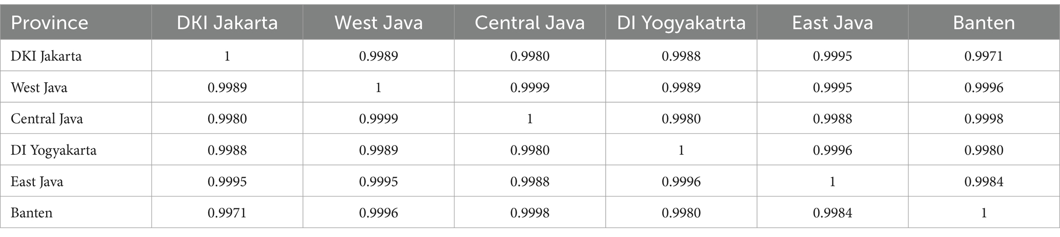
Table 3. Correlations value of the GRDP in six provinces.
As shown in Table 3, the GRDP among the six provinces exhibits high correlation values. This indicates that there is a temporal correlation in the GRDP data, and it suggests that the GRDP of neighboring locations is strongly interrelated.
3.3 Stationarity test
In time series data mode, it is essential to meet certain assumptions, one of which is that the data should be stationary with respect to the mean. The stationarity test for time series data with respect to the mean can be conducted using the augmented Dickey–Fuller (ADF) test. The hypotheses used in the ADF test are as follows:
H0: δ = 1 (Data are not stationary)
H1: δ < 1 (Data are stationary)
H0 is accepted if p-value id < α = 0.05
As shown in Table 4, the GRDP data of the six provinces are not stationary. This is evidenced by the p-values of each province >0.05, indicating that the data do not exhibit stationarity if H0 is accepted; therefore, differencing is required to make the data stationary. The results of the ADF test after differencing twice are shown in Table 5.
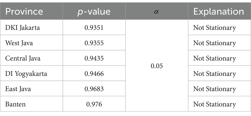
Table 4. ADF test.

Table 5. ADF test after differencing.
After differencing, as shown in Table 5, the GRDP data for all six provinces are stationary. This is evidenced by a p-value in each province <0.05, which means H0 is rejected; hence, the data are stationary.
3.4 Identifying the order of the GSTAR model
Identifying the order of the GSTAR model can be done by examining the plots of the modified autocorrelation function (MACF) and (MPACF) (28). The MACF plot is used to assess the stationarity of the data, while the MPACF plot is used to identify significant lags that can be used as the order of the GSTAR model. Below are the MACF and MPACF plots for the GRDP data.
As shown in Figure 2, the data from the six provinces are stationary, as indicated by the greater number of dots (.) compared with plus (+) and minus (−) symbols. After achieving stationary data for the GRDP in these six provinces, the next step is to determine the order of the GSTAR model. The time order in the GSTAR model can be determined using the MPACF plot, considering the AIC values. Below is the MPACF plot for the GRDP data of the six provinces.
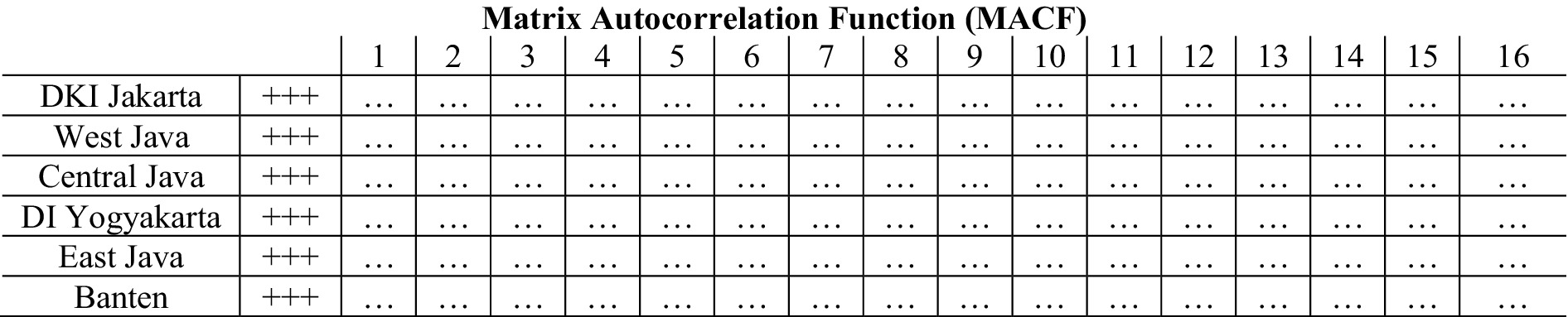
Figure 2. Plot of MACF data GRDP after differencing.
Figure 3 shows that the significant lags are 1, 2, 4, 6, 7, 8, 10, 12, and 14. The next step in selecting the best time order in the GSTAR model is done using the VAR model approach, where the optimal time order is determined based on the smallest AIC value. The AIC values are shown in Table 6 as follows.
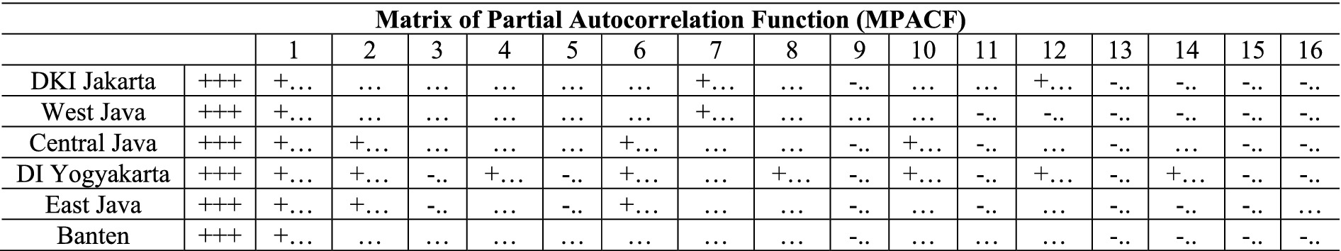
Figure 3. Plot MPACF data GRDP after differencing.
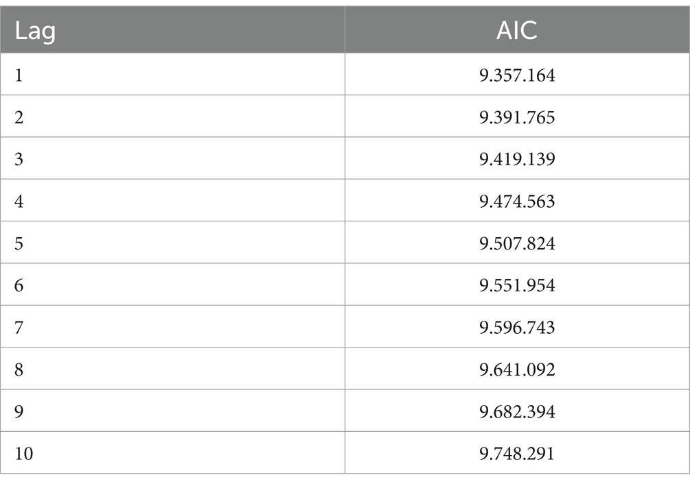
Table 6. AIC value.
Based on Table 6, it is found that the smallest AIC value is associated with lag 1, with a value of 93.57164. Therefore, it can be concluded that the selected autoregressive order (p) for the GSTAR model of the GRDP of six provinces is 1. Thus, the resulting model is GSTAR (11)-I(1).
3.5 Determining location weights
3.5.1 Uniform location weights
Uniform location weights assume that the GRDP of one location has an equal influence on other locations. Based on the cross-correlation between locations at the matrix used in this study, the uniform weight is as follows:
3.5.2 Inverse distance location weights
The determination of inverse distance location weights utilizes the approach of overland transportation distances between provincial capitals. Inverse distance location weights assume that the GRDP data of a location are influenced by the distance between that location and others. Locations that are closer tend to have higher weights compared to those that are farther away. The inverse distance weight matrix is as follows:
3.5.3 Cross-correlation normalized location weights
Based on the order autoregressive (p), the last weight applied in this study is the location corresponding time lag. The corresponding time lag is 1. The matrix of cross-correlation normalization weights is as follows:
3.6 Parameter estimation of the GSTAR-OLS model
Parameter estimation in the GSTAR model can be performed using the least squares method, commonly known as OLS (31). The estimated parameter values are considered significant if . Here are the results of the significance test of the GSTAR (11)-I(1) model parameters of the six locations using uniform, inverse distance, and cross-correlation normalization weights.
3.6.1 Significance test of the GSTAR (11)-I(1) model with uniform weights
The results of the significance test of the GSTAR (11)-I(1) model parameters using uniform weights are shown in Table 7 as follows.
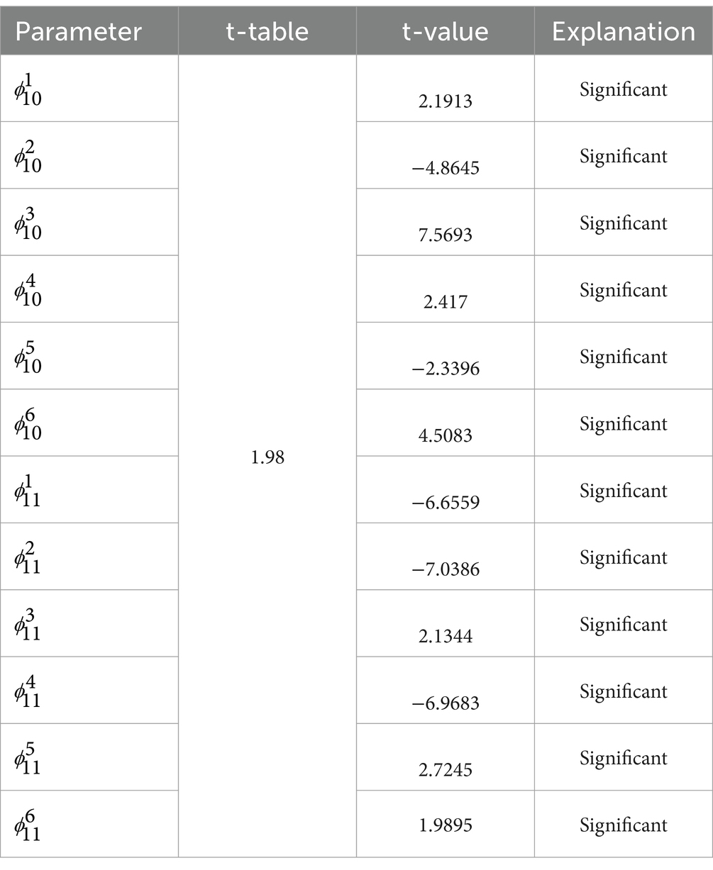
Table 7. Significance test of the GSTAR (11)-I(1) with uniform weights.
3.6.2 Significance test of the GSTAR (11)-I(1) with inverse distance weights
The results of the significance test of the GSTAR (11)-I(1) model parameters using inverse distance weights are shown in Table 8 as follows.
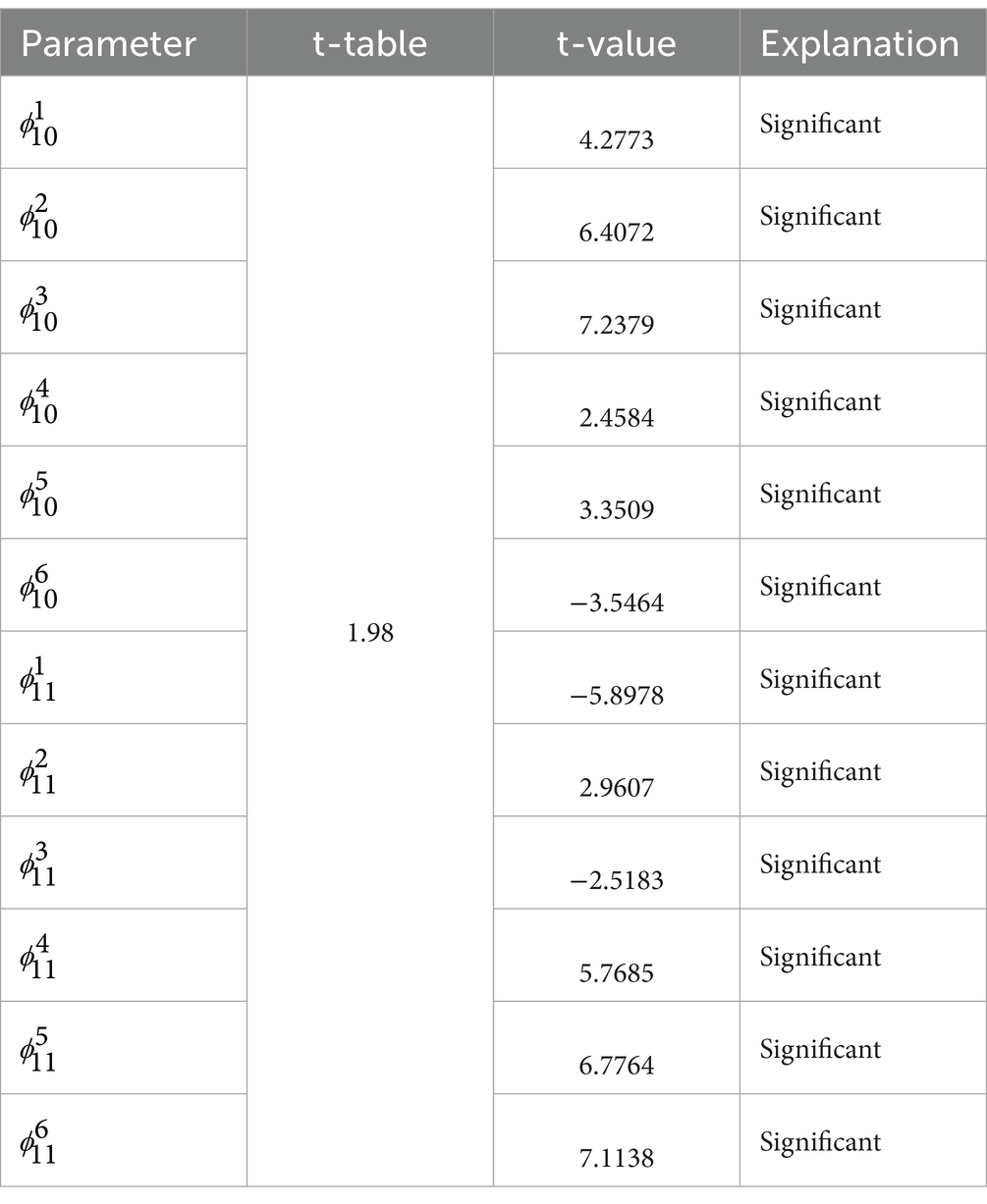
Table 8. Significance test of the GSTAR (11)-I(1) with inverse distance weights.
3.6.3 Significance test of the GSTAR (11)-I(1) with normalized cross-correlation weights
The results of the significance test of the GSTAR model (11)-I(1) using cross-correlation normalization weights are shown in Table 9 as follows.
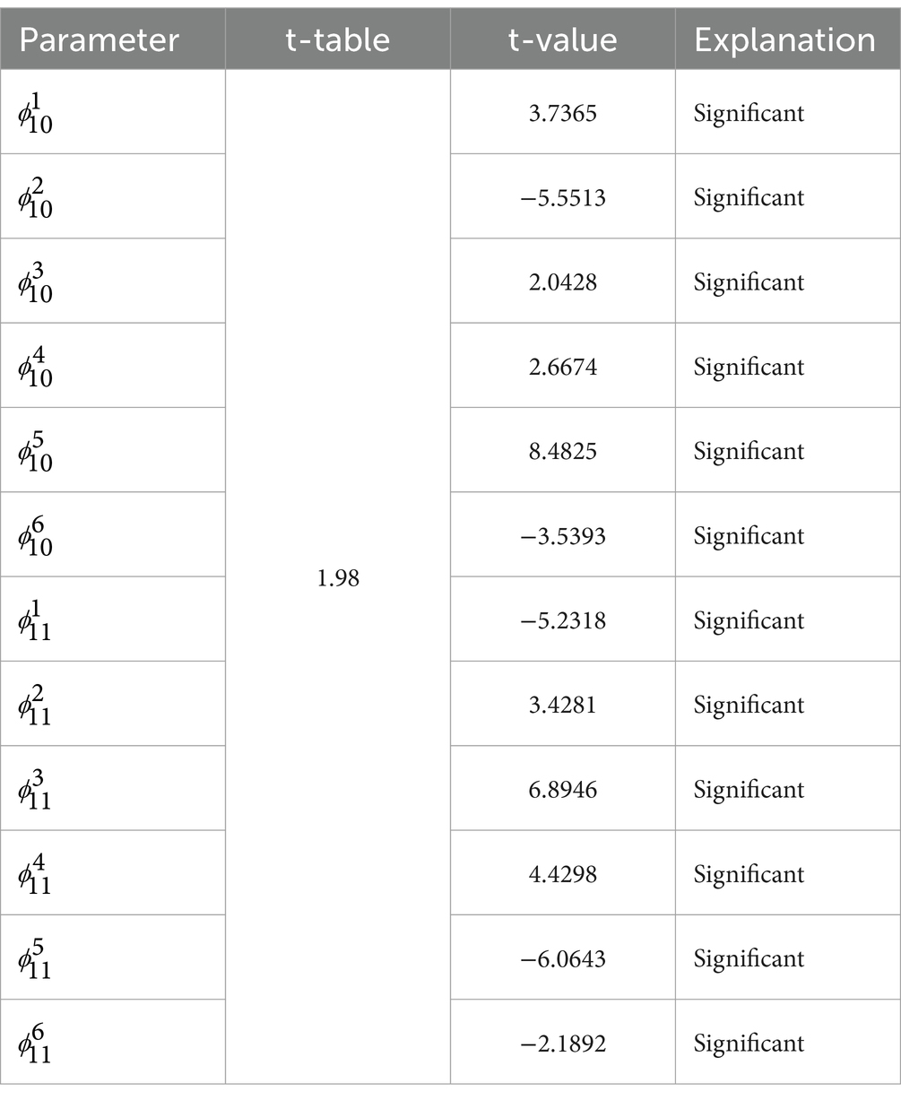
Table 9. Significance test of the GSTAR (11)-I(1) with normalized cross-correlation weights.
3.7 Testing residual correlations between locations
Before modeling the GSTAR Model (11)-I(1) using SUR, a Lagrange multiplier test is conducted to determine whether there is a residual correlation between locations in the GSTAR model (11)-I(1). Below is the Lagrange multiplier test.
The hypotheses are as follows:
H0 = for all (heteroskedasticity in the variance–covariance structure of residuals and correlation between residual equations).
H1 = for all (heteroskedasticity in the variance–covariance structure of residuals and correlation between residual equations).
Significance level:
Test criteria:
Test statistics:
Here are the Lagrange multiplier test statistics for each weight type.
In this research, as shown in Table 10, it was found that the GSTAR model (11)-I(1) for all the weights exhibits residual correlation between locations. Therefore, using OLS estimates, the GSTAR model may not be suitable for forecasting. OLS estimation methods for GSTAR models with correlated residuals can yield less efficient estimators due to the increased likelihood of larger errors during forecasting. As a result, a new modeling approach was used by SUR with GLS estimates to achieve more efficient parameter estimations.
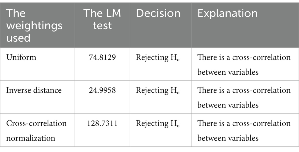
Table 10. Lagrange multiplier test.
3.8 Estimation of GSTAR-SUR model parameters using the GLS method
After conducting the Lagrange multiplier test, the model with correlated residuals is further processed using the GSTAR-SUR model. The estimation of model parameters in the GSTAR-SUR model can be done using the GLS method. In this phase, we use Python (32). The assessment of significant parameter estimates in this method is similar to the GSTAR model, meaning that a parameter estimate is considered significant if . However, in this particular study, non-significant parameters were not eliminated to ensure that the weighting of each location remained stable. Below are the parameter estimates of the GSTAR-SUR model for all six locations based on each weighting.
3.9 Estimation of GSTAR-SUR model parameters (11)-I(1) with distance weight
The results of estimating GSTAR model parameters (11)-I(1) using inverse distance weights are shown in Table 11 as follows.
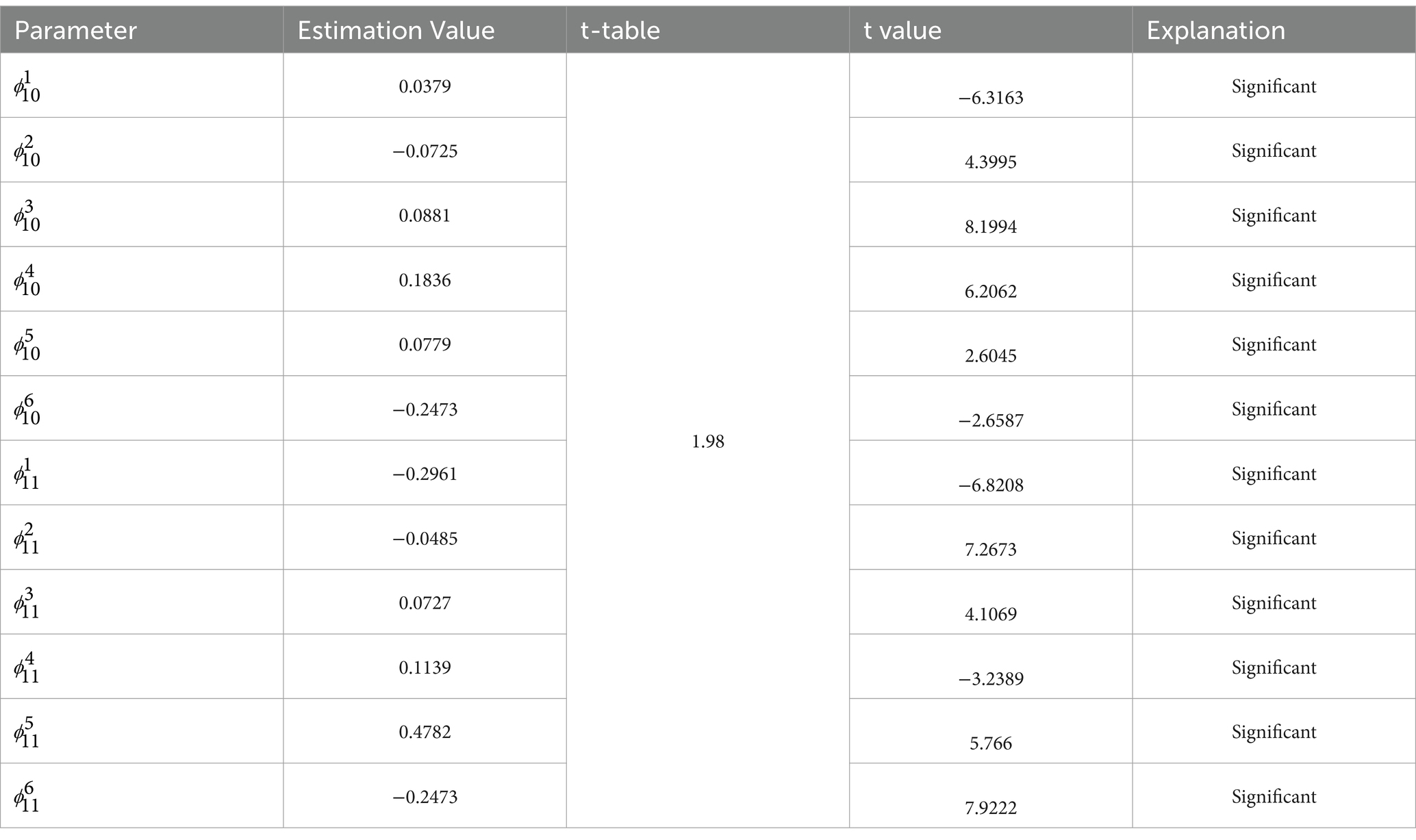
Table 11. Parameter estimation in GSTAR-SUR (11)-I(1) with inverse distance.
Based on these parameters, the matrix equation for the GSTAR model is (1.1) when using uniform weights. The model can be formulated as follows:
or
Therefore, the GSTAR model obtained (11)-I(1) using inverse distance weights for each location can be represented as follows:
1. The equation model of GSTAR (11)-I(1) for GRDP DKI Jakarta is as follows:
2. The equation model of GSTAR (11)-Im (1) for GRDP West Java is as follows:
3. The equation model of GSTAR (11)-I(1) for GRDP Central Java is as follows:
4. The equation model of GSTAR (11)-I(1) for GRDP DI Yogyakarta is as follows:
5. The equation model of GSTAR (11)-I(1) for GRDP East Java is as follows:
6. The equation model of GSTAR (11)-I(1) for GRDP Banten is as follows:
3.10 Model GSTAR-SUR feasibility test (11)-I(1)
After finding the parameters and models for each location, the next step is to test the white noise assumption for the residuals. Checking this assumption aims to determine whether the residuals from each equation are independent of each other. The method used to assess the white noise assumption is the Ljung–Box test, and the results of the Ljung–Box test are shown in Table 12.
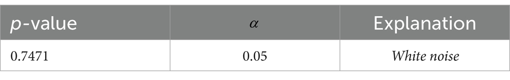
Table 12. The results of the white noise test.
Based on Table 12, it can be observed that all the p-values of the Ljung–Box test for each weight are greater than =0.05, meaning that the residuals in the model meet the white noise assumption. Therefore, it can be concluded that the model is suitable for forecasting.
3.11 Evaluation of the GSTAR-SUR model (11)-I(1)
After attaining the GSTAR-SUR model and conducting model feasibility tests, the next step is to calculate the forecast accuracy of the model by examining the MAPE value. The calculated MAPE value for the GSTAR-SUR model is 8.451%. Consequently, it can be concluded that the GSTAR-SUR model (11)-I(1) demonstrates a high level of accuracy.
3.12 Forecasting GRDP data for each municipality using the optimal model
The best model that has been obtained is GSTAR-SUR (11)-I(1) inverse distance weight. This model is used for forecasting to obtain predictions of the GRDP data for the six provinces on Java Island, namely, Banten, DKI Jakarta, West Java, Central Java, East Java, and DI Yogyakarta. Data forecasting is performed for 7 quarters. The forecasting results are shown in Table 13 as follows.

Table 13. Forecasted GRDP results for the next seven quarters.
As shown in Table 13, it is observed that the forecasted GRDP values of all six provinces for the next 7 quarters until December 2024 will experience a monthly increase.
However, the GRDP growth remains relatively stable, as there are no significant spikes from 1 month to the next month. The forecasted results are shown in Figure 4 as follows.
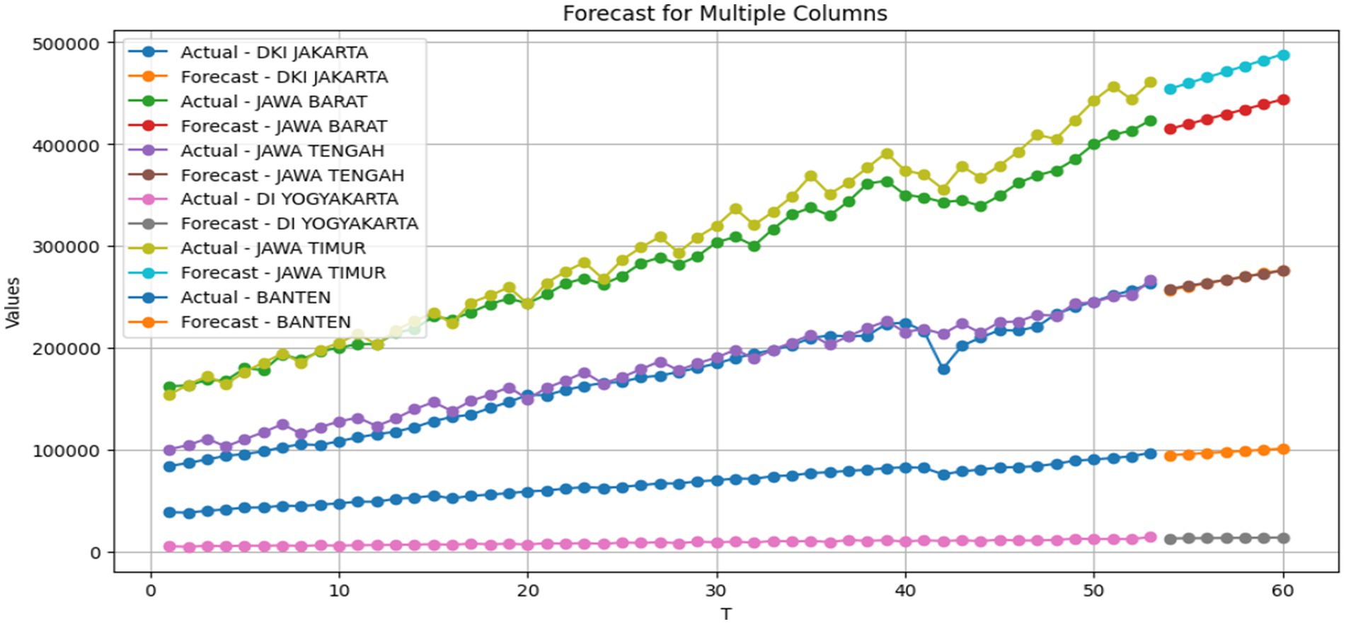
Figure 4. Forecasted GRDP from January 2024 to December 2024.
The forecasted data plot indicates that the GRDP data for the next 7 quarters in all six provinces follow a trend pattern. This is evident from the increasing trend in the GRDP values for each month.
4 Discussion
The data obtained from the GRDP variable contain spatial and temporal information, requiring an appropriate model to forecast spatiotemporal data, namely, the GSTAR model. In this research, it was found that the GSTAR model (11)-I(1) for all the weights exhibits residual correlation between locations; hence, the GSTAR model using OLS estimates may not be suitable for forecasting. This is supported by the research conducted by Adella et al. (20) with a case study of the number of tourists in Central Java, which produced the GSTAR model (2.1), and there was a correlation between residuals. Moreover, it was continued using the GSTAR-SUR method. The SUR model is a multivariate linear regression model in which the errors are uncorrelated within a single equation but are correlated across equations (16). As a result, a new modeling approach was used by SUR with GLS estimates to achieve more efficient parameter estimations. After conducting the Lagrange multiplier test, the optimal model is GSTAR-SUR (11)-I(1) with inverse distance location weights, demonstrating high accuracy with a MAPE value of 8.451%. Forecasts for Banten, DKI Jakarta, West Java, Central Java, East Java, and DI Yogyakarta predict consistent monthly GRDP increases in December 2024.
5 Conclusion
The best model that has been obtained is GSTAR-SUR (11)-I(1) with inverse distance location weights. The calculated MAPE value for the GSTAR-SUR model is 8.451%. Consequently, it can be concluded that the GSTAR-SUR model (11)-I(1) demonstrates a high level of accuracy. The best model that has been obtained is GSTAR-SUR (11)-I(1) with inverse distance weight. This model is then used for forecasting to obtain predictions of the GRDP data for the six provinces on Java Island, namely, Banten, DKI Jakarta, West Java, Central Java, East Java, and DI Yogyakarta. The forecasted GRDP values of all six provinces for the next 7 quarters until December 2024 will experience a monthly increase. However, the GRDP growth remains relatively stable, as there are no significant spikes from 1 month to the next.
Data availability statement
The datasets presented in this study can be found in online repositories. The names of the repository/repositories and accession number(s) can be found at: BPS Java Island.
Author contributions
PR: Conceptualization, Data curation, Formal analysis, Funding acquisition, Investigation, Software, Methodology, Project administration, Resources, Supervision, Validation, Visualization, Writing – original draft, Writing – review & editing. IF: Data curation, Project administration, Resources, Software, Writing – original draft. SA: Project administration, Resources, Visualization, Writing – review & editing.
Funding
The author(s) declare that no financial support was received for the research, authorship, and/or publication of this article.
Acknowledgments
The authors thank the Department of Statistics and the Department of Data Science for being an integral part of the Faculty of Science and Agriculture Technology at Universitas Muhammadiyah Semarang. Their substantial support and dedication in advancing this research to completion are immensely valued. The authors would also like to thank Universitas Muhammadiyah Semarang for the provision of resources, facilities, and academic guidance, which have been pivotal in supporting our research.
Conflict of interest
The authors declare that the research was conducted in the absence of any commercial or financial relationships that could be construed as a potential conflict of interest.
Publisher’s note
All claims expressed in this article are solely those of the authors and do not necessarily represent those of their affiliated organizations, or those of the publisher, the editors and the reviewers. Any product that may be evaluated in this article, or claim that may be made by its manufacturer, is not guaranteed or endorsed by the publisher.
References
1. Hajeri, EY, and Dolorosa, E. Analisis Penentuan Sektor Unggulan Perekonomian di Kabupaten Kubu Raya. Jurnal Ekonomi Bisnis dan Kewirausahaan. (2015) 4:253–26. doi: 10.26418/jebik.v4i2.12485
3. BPS. “Laporan Perekonomian Indonesia Tahun 2022,” Available at: www.freepik.com (2022).
4. Cryer, J. D., and Chan, K.-S. “Springer Texts in Statistics Time Series Analysis With Applications in R Second Edition.” (2008).
5. Mubarok, M. H. “Peramalan Cuaca di Stasiun Meteorologi Klas I Djuanda Surabaya Menggunakan Metode Arima dan Vector Autoregresive (VAR).” (2015).
6. Nofitasari, D, Priyono, TH, and Yuliati, L. Analisis PDRB Sektor Industri Dengan Pendekatan Regresi Spsial: Studi Kasus Indonesia 2011-1015. Media Trend. (2018) 13:90. doi: 10.21107/mediatrend.v13i1.3591
7. Akbar, MS, Setiawan, N, Suhartono, A, Ruchjana, BN, Prastyo, DD, Muhaimin, A, et al. A Generalized Space-Time Autoregressive Moving Average (GSTARMA) Model for Forecasting Air Pollutant in Surabaya. J Phys Conf Ser. (2020) 1490:012022. doi: 10.1088/1742-6596/1490/1/012022
8. Alawiyah, M, Kusuma, DA, and Ruchjana, BN. Model Space Time Autoregressive Integrate (STARI) Untuk Data ebit Air Sungai Citarum Di Provinsi Jawa Barat (Space Time Autoregressive Integrated (STARI) Model for Citarum River Water Discharge Data in West Java Province). Jurnal Ilmu Matematika dan Terapan. (2020) 14:147–58. doi: 10.30598/barekengvol14iss1pp147-158
9. Ruchjana, B. N. “A Generalized Space-time Autoregressive Model and Its Application to oil production.” (2002).
10. Wijaya, FB, and Made Sumertajaya, I. Comparison of Autoregressive (AR), Vector Autoregressive (VAR), Space Time Autoregressive (STAR), and Generalized Space Time Autoregressive (GSTAR) in Forecasting (Case: Simulation study with Autoregressive pattern). Int J Appl Eng Res. (2015) 10:42388–95.
11. Sulistyono, AD, Hartawati, H, Suryawardhani, NW, Iriany, A, and Iriany, A. Cross-Covariance Weight of GSTAR-SUR Model for Rainfall Forecasting in Agricultural Areas. Jurnal Matematika Murni dan Aplikasi. (2020) 6:49–57. doi: 10.18860/ca.v6i2.7544
12. Fransiska, H, Sunandi, E, and Agustina, D. Peramalan Curah Hujan Provinsi Bengkulu dengan Generalized Space-Time Autoregressive. J Maths Educ Sci Technol. (2020) 5:130. doi: 10.30651/must.v5i2.5326
13. Huda, NM, and Imro’ah, N. Determination of the best weight matrix for the Generalized Space Time Autoregressive (GSTAR) model in the Covid-19 case on Java Island, Indonesia. Spat Stat. (2023) 54:100734. doi: 10.1016/j.spasta.2023.100734
14. Borovkova, S, Lopuhaä, HP, and Ruchjana, BN. Consistency and asymptotic normality of least squares estimators in generalized STAR models. Statistica Neerlandica. (2008) 62:482–508. doi: 10.1111/j.1467-9574.2008.00391.x
15. Zellner, A. An Efficient Method of Estimating Seemingly Unrelated Regressions and Tests for Aggregation Bias. J Am Stat Assoc. (1962) 57:348–68. doi: 10.1080/01621459.1962.10480664
16. Setiawan, S., Suhartono, S., Prastuti, M., Setiawan, S., and Prastuti, M., “S-GSTAR-SUR model for seasonal spatio temporal data forecasting,” Available at: http://einspem.upm.edu.my/journal (2016).
17. Tiong, KY, Ma, Z, and Palmqvist, CW. Analyzing factors contributing to real-time train arrival delays using seemingly unrelated regression models. Transp Res Part A Policy Pract. (2023) 174:103751. doi: 10.1016/j.tra.2023.103751
18. Yundari, GH, and Perdana, H. Penerapan GSTAR-SUR Pada Jumlah Peumpang Pesawat Domestik Di Bandara Indonesia. Buletin Ilmiah Matematika, Statistika dan Terapannya. (2020) 9:275–84. doi: 10.26418/bbimst.v9i2.39919
19. Septyaningrum, W. P. I. “Peramalan Jumlah Wisatawan Pada Tiga Lokasi Wisata Di Kabupaten Pacitan Menggunkan Metode GSTAR-SUR.” (2017).
20. Adella, I, Ispriyanti, D, and Yasin, H. Pemodelan Jumlah Wisatawan Di Jawa Tengah Menggunakan Metode Generalized Space Time Autoregressive-Seemingly Unrelated Regression (GSTAR-SUR). J Gaussian. (2022) 11:258–65. doi: 10.14710/j.gauss.v11i2.35473
21. Hapsari, R. “Pengembangan Ramalan Interval Pada Model GSTARX Utuk Peramalan Indeks Harga Konsumen Kelompok Bahan Makanan.” (2017).
22. Harini, S., and Nuronia, N., “Determination of consumer price index with generalized space-time autoregressive,” In IOP Conference Series: Earth and Environmental Science, Institute of Physics Publishing. (2020).
23. Hassani, H, and Thomakos, D. A review on singular spectrum analysis for economic and financial time series. Stat Interface. (2010) 3:377–97. doi: 10.4310/sii.2010.v3.n3.a11
24. Pfeifer, PE, and Deutsch, SJ. A Three-Stage Iterative Procedure for Space-Time Modeling. Technometrics. (1980) 22:35. doi: 10.2307/1268381
25. Islamiyah, AN, Rahayu, W, and Wiraningsih, ED. Pemodelan Generalized Space Time Autoregressive (GSTAR) dan Penerapannya pada Penderita TB Paru (BTA+) di DKI Jakarta. Jurnal Statistika dan Aplikasinya. (2018) 2:36–48. doi: 10.21009/JSA.02205
26. Kurata, H. On the Efficiencies of Several Generalized Least Squares Estimators in a Seemingly Unrelated Regression Model and a Heteroscedastic Model. J Multivar Anal. (1999) 70:86–94. doi: 10.1006/jmva.1999.1817
27. Matsuura, S, and Kurata, H. Optimal estimator under risk matrix in a seemingly unrelated regression model and its generalized least squares expression. Stat Pap. (2022) 63:123–41. doi: 10.1007/s00362-021-01232-5
28. Wei, W. W. S., “Writing a Book on Multivariate Time Series Analysis and its Applications View project,” (2006). Available at: https://www.researchgate.net/publication/236651810
29. Khair, U, Fahmi, H, Al Hakim, S, and Rahim, R. Forecasting Error Calculation with Mean Absolute Deviation and Mean Absolute Percentage Error. J Phys Conf Ser. (2017) 930:12002. doi: 10.1088/1742-6596/930/1/012002
30. Khoerunnisa, A., Manfaati Nur, I., and Arum, P. R., “Metode Markov Switching Autoregressive (MSAR) untuk Peramalan Indeks Saham Syariah Indonesia (ISSI) Markov Switching Autoregressive (MSAR) Method for Forecasting Indonesian Islamic Stock Index (ISSI).” (2022).
31. Zaenal, A., and Revadiansyah, F., “gstar: Generalized Space-Time Autoregressive Model.” Available at: https://CRAN.R-project.org/package=gstar (2019).
Keywords: GRDP, Java Island, GSTAR, SUR, GSTAR-SUR
Citation: Rismawati Arum P, Fathoni Amri I and Amri S (2024) GLS estimation in python to forecast gross regional domestic product using generalized space–time autoregressive seemingly unrelated regression model. Front. Appl. Math. Stat. 10:1365723. doi: 10.3389/fams.2024.1365723
Edited by:
Maria Cristina Mariani, The University of Texas at El Paso, United StatesReviewed by:
Yu Mu, Stony Brook University, United StatesDragos Bozdog, Stevens Institute of Technology, United States
Copyright © 2024 Rismawati Arum, Fathoni Amri and Amri. This is an open-access article distributed under the terms of the Creative Commons Attribution License (CC BY). The use, distribution or reproduction in other forums is permitted, provided the original author(s) and the copyright owner(s) are credited and that the original publication in this journal is cited, in accordance with accepted academic practice. No use, distribution or reproduction is permitted which does not comply with these terms.
*Correspondence: Prizka Rismawati Arum, cHJpemthLnJpc21hd2F0aWFydW1AdW5pbXVzLmFjLmlk