Wave Effects of the Fractional Shallow Water Equation and the Fractional Optical Fiber Equation

The non-linear space-time fractional Estevez-Mansfield-Clarkson (EMC) equation and the non-linear space-time fractional Ablowitz-Kaup-Newell-Segur (AKNS) equation showed the motion of waves in the shallow water equation and the optical fiber equation, respectively. The process used to solve these equations is to transform the non-linear fractional partial differential equations (PDEs) into the non-linear ordinary differential equations by using the Jumarie's Riemann-Liouville derivative and setting the solution in the finite series combined with the simple equation (SE) method with the Bernoulli equation. The new traveling wave solutions were the exponential functions resulting in the physical wave effects are produced in the form of kink waves and represented by the two-dimensional graph, three-dimensional graph, and contour graph. In addition, the comparison of the solutions revealed that the new solutions have a more convenient and easier format.

1. Introduction

The partial differential equations (PDEs) are very important in studying and explaining the phenomena of mathematical physics. The most widely used scenarios are plasma physics, optical fibers, fluid mechanics, solid state physics, plasma waves, capillary-gravity waves, and water waves. At present, the researchers are interested in studying the exact solutions or the numerical solutions [1–3] in order to apply the results obtained in the above studies. To study the effects of these matters more closely, it is necessary to study the form of the exact traveling wave solution of non-linear fractional PDEs. There are a variety of methods to solve non-linear fractional PDEs such as generalized Kudryashov method [4, 5], extended Kudryashov method [6], modified Kudryashov method [7, 8], first integral method [9–11], G′/G-expansion method [12–14], fractional sub-equation method [15–17], and Poincar$\acute{\mathrm{\text{e}}}$-Lighthill-Kuo method [18, 19].

In 2006, the Jumarie's Riemann-Liouville derivative [20] was given as follows,

$\begin{array}{ll}{D}_t^{\alpha }f(t)=\{\begin{array}{ll}f(t)\hfill & ,\alpha \text{ = 0}\hfill \\ \frac{1}{\Gamma (1-\alpha )}\frac{d}{dt}{\displaystyle {\int }_0^t{(t-\psi )}^{-\alpha }}[f(\psi )-f(0)]d\psi \hfill & ,\text{0}<\alpha <\text{1}\hfill \\ \frac{d^n}{d{t}^n}{D}_t^{\alpha -n}f(t)\hfill & ,\text{n}\le \alpha <n\text{+1},n\ge \text{1},\hfill \end{array}& (1)\end{array}$

where α is an order of the fractional derivative.

The important properties of fractional Riemann-Liouville derivatives [21] were discovered in 2009 as follows,

$\begin{array}{ll}{D}_t^{\alpha }{t}^k=\frac{\Gamma (k+1)}{\Gamma (k-\alpha +1)}{t}^{(k-\alpha )},k\ge 0,& (2)\end{array}$

$\begin{array}{ll}{D}_t^{\alpha }\left[f(t)g(t)\right]=f(t)D_t^{\alpha }g(t)+g(t)D_t^{\alpha }f(t),& (3)\end{array}$

$\begin{array}{ll}{D}_t^{\alpha }f\left[g(t)\right]=D_g^{\alpha }f\left[g(t)\right]{\left[g^{\prime }(t)\right]}^{\alpha }=f_g^{\prime }\left[g(t)\right]D_t^{\alpha }g(t).& (4)\end{array}$

Mansfield and Clarkson [22] introduced the Estevez-Mansfield-Clarkson (EMC) equation in 1997. This equation was applied to understand the non-linear dispersion of patterns in liquid drops. Zhen-Ya [23] suggested the two-parameter family of fully EMC equation E(m, n) in 2002 as follows,

$\begin{array}{ll}{(u_y^m)}_{yyt}+\delta {(u_y^n{u}_t)}_y+u_{tt}=0& (5)\end{array}$

where δ is a constant. If (m, n) = (1, 1) then Equation (5) reduces to the EMC equation

$\begin{array}{ll}{u}_{yyyt}+\delta u_y{u}_{yt}+\delta u_{yy}{u}_t+u_{tt}=0.& (6)\end{array}$

In 1970, Ablowitz, Kaup, Newell, and Segur [24] purposed the Ablowitz-Kaup-Newell-Segur (AKNS) equations which were motivated by the applications to non-linear optics. The AKNS equation can be reduced to some non-linear evolution equations such as the non-linear Schr$\ddot{\mathrm{\text{o}}}$dinger, the sine-Gordon equations, the kdV equation, and others. The fourth-order non-linear AKNS equation with the parameter β in this form,

$\begin{array}{ll}4u_{xt}+u_{xxxt}+8u_x{u}_{xy}+4u_{xx}{u}_y-\beta u_{xx}=0.& (7)\end{array}$

In this article, we have solved the non-linear space-time fractional EMC equation and the non-linear space-time fractional AKNS equation by applying Jumarie's Riemann-Liouville derivative and the SE method with the Bernoulli equation. We have shown the new exact solutions and the wave effects in a two-dimensional graph, three-dimensional graph, and contour graph. Finally, we have compared the new solutions with some effective articles [25] to show that our solutions had a more convenient and simpler form.

2. Algorithm of SE Method

In this section, we discuss the SE method with the Bernoulli Equation [26] for solving fractional PDEs. The general form of fractional PDEs is shown as

$\begin{array}{l}G(u,D_x^{\alpha }u,D_y^{\alpha }u,D_t^{\alpha }u,D_x^{2\alpha }u,D_y^{\alpha }{D}_x^{\alpha }u,D_t^{\alpha }{D}_x^{\alpha }u,\dots )=0,t>0,\\ 0<\alpha \le 1.& (8)\end{array}$

This method is described in the following steps,

Step 1. Wave transformationThe traveling wave solution of fractional PDEs is a solution that satisfies

$\begin{array}{ll}u(x,y,t)=U(\psi ),\psi =\frac{k{x}^{\alpha }}{\Gamma (\alpha +1)}+\frac{l{y}^{\alpha }}{\Gamma (\alpha +1)}-\frac{c{t}^{\alpha }}{\Gamma (\alpha +1)},& (9)\end{array}$

where ψ is a general term for a traveling wave, c is a wave velocity constant. We called stationary wave when c = 0. For c>0, the wave moves in the positive direction, and for c < 0, the wave moves in the negative direction [27]. Reducing Equation (8) into an ODE,

$\begin{array}{ll}Q\left(U,\frac{dU}{d\psi },\frac{d^{2}U}{d{\psi }^2},\frac{d^{3}U}{d{\psi }^3},\dots \right)=0,& (10)\end{array}$

where Q is a polynomial in U(ψ) and its derivatives.

Step 2. Solution suppositionThe solution of Equation (10) can be written in the finite series,

$\begin{array}{ll}U(\psi )={\displaystyle \sum _{i=0}^N}{a}_i{H}^i(\psi ),& (11)\end{array}$

where a_i are real constants with a_N≠0 and H(ψ) depends on the simple equation (SE) method with Bernoulli equation which states as follows.

$\begin{array}{ll}{H}^{\prime }(\psi )=\mu H(\psi )+\eta H^2(\psi )& (12)\end{array}$

where μ and η are the non-zero constant. The solutions of Equation (12) have two cases with ψ₀ as an integration constant,

Case 1 : μ > 0, η < 0,

$\begin{array}{ll}H(\psi )=\frac{\mu e^{\mu (\psi +{\psi }_0)}}{1-\eta e^{\mu (\psi +{\psi }_0)}}.& (13)\end{array}$

Case 2 : μ < , η > 0,

$\begin{array}{ll}H(\psi )=-\frac{\mu e^{\mu (\psi +{\psi }_0)}}{1+\eta e^{\mu (\psi +{\psi }_0)}}.& (14)\end{array}$

Step 3. Finding the integer NBalance the highest order derivative and non-linear terms in Equation (10) to get the integer N in Equation (10).

Step 4. Solution obtaining

Find the parameters a_i, (i = 1, 2, 3, …, N) and c by collecting the coefficients all terms with the same order of Hⁱ, (i = 1, 2, 3, …, N) and setting them to zero [28]. Hence, we constitute the analytical solutions of Equation 10.

3. Applications

We present the traveling wave effects of the non-linear space-time fractional EMC equation and the non-linear space-time fractional AKNS equation.

3.1. The Space-Time Fractional EMC Equation

The fourth-order non-linear space-time fractional EMC Equations [22, 25] is stated as follows,

$\begin{array}{ll}{D}_y^{3\alpha }{D}_t^{\alpha }u+\delta D_y^{\alpha }u{D}_y^{\alpha }{D}_t^{\alpha }u+\delta D_y^{2\alpha }u{D}_t^{\alpha }u+D_t^{2\alpha }u=0,t>0,0<\alpha \le 1,& (15)\end{array}$

where u = u(x, y, t) and δ is constant. Supposing the solution u(x, y, t) = U(ψ) and applying the transformation

$\begin{array}{ll}\psi =\frac{k{x}^{\alpha }}{\Gamma (\alpha +1)}+\frac{l{y}^{\alpha }}{\Gamma (\alpha +1)}-\frac{c{t}^{\alpha }}{\Gamma (\alpha +1)},& (16)\end{array}$

where k, l, and c are non-zero constants. The Equation (15) changed into an ODE,

$\begin{array}{ll}-l^3\frac{d^{4}U}{d{\psi }^4}-2l^2\delta \frac{dU}{d\psi }·\frac{d^{2}U}{d{\psi }^2}+c\frac{d^{2}U}{d{\psi }^2}=0.& (17)\end{array}$

Integrating Equation (17) with zero constant, we get

$\begin{array}{ll}-l^3\frac{d^{3}U}{d{\psi }^3}-l^2\delta {\left(\frac{dU}{d\psi }\right)}^2+c\frac{dU}{d\psi }=0.& (18)\end{array}$

Using the SE method. The solution was set in the form of Equation (11). Next, we balanced the non-linear terms and the highest order derivative of Equation (18). Thus, N = 1. The Equation (11) turned into

$\begin{array}{ll}U(\psi )=a_0+a_{1}H(\psi ).& (19)\end{array}$

Replacing Equation (18) with Equation (19). We collected all terms of the same power of H(ψ) and set each coefficient to zero as follows,

$\begin{array}{lll}{H}^1(\psi ):& -a_1{l}^3{\mu }^3+a_{1}c\mu =0,& (20)\end{array}$

$\begin{array}{lll}{H}^2(\psi ):& -7a_1{l}^3{\mu }^2\eta -a_1^2{l}^2\delta {\mu }^2+a_{1}c\eta =0,& (21)\end{array}$

$\begin{array}{lll}{H}^3(\psi ):& -12a_1{l}^3\mu {\eta }^2-2a_1^2{l}^3\delta \mu \eta =0,& (22)\end{array}$

$\begin{array}{lll}{H}^4(\psi ):& -6a_1{l}^3{\eta }^3-a_1^3{l}^2\delta {\eta }^2=0.& (23)\end{array}$

Solving the system of Equations (20)–(23), we get

$\begin{array}{ll}{a}_1=\frac{-6l\eta }{\delta },c=l^3{\mu }^2.& (24)\end{array}$

By Equations (13), (14), (16), and (24), the exact traveling wave solutions of the non-linear space-time fractional EMC equations are represented in two cases with arbitrary constant ψ₀:

Case I: μ>0, η <0,

$\begin{array}{ll}u\left(x,y,t\right)=a_0-\frac{6l\eta }{\delta }\left(\frac{\mu e^{\mu (\psi +{\psi }_0)}}{1-\eta e^{\mu (\psi +{\psi }_0)}}\right),& (25)\end{array}$

Case II: μ <0, η>0,

$\begin{array}{ll}u(x,y,t)=a_0+\frac{6l\eta }{\delta }\left(\frac{\mu e^{\mu (\psi +{\psi }_0)}}{1+\eta e^{\mu (\psi +{\psi }_0)}}\right),& (26)\end{array}$

where $\psi =\frac{k{x}^{\alpha }}{\Gamma (\alpha +1)}+\frac{l{y}^{\alpha }}{\Gamma (\alpha +1)}-\frac{l^3{\mu }^2{t}^{\alpha }}{\Gamma (\alpha +1)}$.

Next, we present the example graph of wave effects of the non-linear space-time fractional EMC equation by setting some parameter to obtain proper graph. Equation (25) shows the exact exponential solutions which forms a kink wave effect, increasing from one state to another, with a₀ = 0, δ = 1, k = 1, l = 1, μ = 1, η = −1, α = 0.5, 0 ≤ x ≤ 90, 0 ≤ y ≤ 90, and t = 200, 400 shown in Figure 1. We set the parameters a₀ = 0, δ = 1, k = 1, l = 1, μ = −1, η = 1, α = 0.5, 0 ≤ x ≤ 90, 0 ≤ y ≤ 90, and t = 100, 300 into an Equation (26), kink wave effect shown in Figure 2.

FIGURE 1

Figure 1. Kink wave solution of Equation (25) in 3D, contour and 2D for Case I.

FIGURE 2

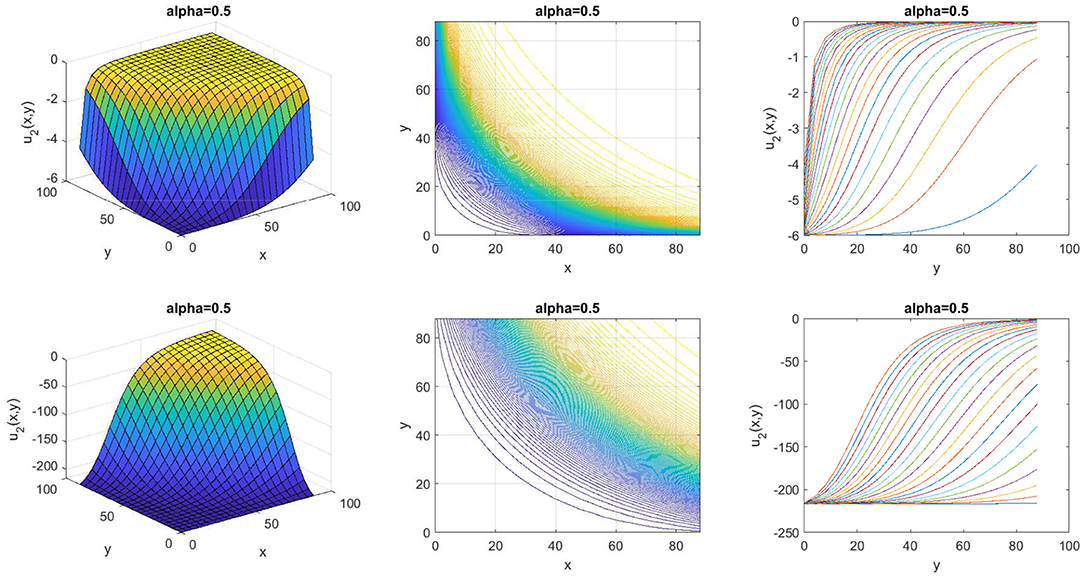
Figure 2. Kink wave solution of Equation (26) in 3D, contour and 2D for Case II.

3.2. The Space-Time Fractional AKNS Equation

The fourth-order non-linear space-time fractional AKNS equation is defined as follows [25],

$\begin{array}{l}4D_x^{\alpha }{D}_t^{\alpha }u+D_x^{3\alpha }{D}_t^{\alpha }u+8D_x^{\alpha }u{D}_x^{\alpha }{D}_y^{\alpha }u+4D_x^{2\alpha }u{D}_y^{\alpha }u-\beta D_x^{2\alpha }u=\\ 0,t>0,0<\alpha \le 1,& (27)\end{array}$

where u = u(x, y, t) and β is constant. Similar to the previous equation, we set the solution and transform Equation (27) by Equation (16), we obtain

$\begin{array}{l}-4ck\frac{d^{2}U}{d{\psi }^2}-c{k}^3\frac{d^{4}U}{d{\psi }^4}+8k^{2}l\frac{dU}{d\psi }·\frac{d^{2}U}{d{\psi }^2}+4k^{2}l\frac{dU}{d\psi }·\frac{d^{2}U}{d{\psi }^2}-\beta k^2\frac{d^{2}U}{d{\psi }^2}=0\\ -(4c+\beta k)\frac{d^{2}U}{d{\psi }^2}-c{k}^2\frac{d^{4}U}{d{\psi }^4}+12kl\frac{dU}{d\psi }·\frac{d^{2}U}{d{\psi }^2}=0.& (28)\end{array}$

Integrating Equation (28) and set constant to zero,

$\begin{array}{ll}-(4c+\beta k)\frac{dU}{d\psi }-c{k}^2\frac{d^{3}U}{d{\psi }^3}+6kl{\left(\frac{dU}{d\psi }\right)}^2=0.& (29)\end{array}$

Balancing Equation (29), we got N = 1. Thus, Equation (11) changed to

$\begin{array}{ll}U(\psi )=a_0+a_{1}H(\psi ).& (30)\end{array}$

Replacing Equation (29) with Equation (30). Collecting all terms which have the same power of H(ψ). Setting each coefficient of them to zero, we have

$\begin{array}{lll}{H}^1(\psi ):& -a_{1}c\mu -a_1\beta k\mu -a_{1}c{k}^2{\mu }^3=0,& (31)\end{array}$

$\begin{array}{lll}{H}^2(\psi ):& -4a_{1}c\eta -a_1\beta k\eta -7a_{1}c{k}^2{\mu }^2\eta +6a_1^{2}kl{\mu }^2=0,& (32)\end{array}$

$\begin{array}{lll}{H}^3(\psi ):& -12a_{1}c{k}^2\mu {\eta }^2+12a_1^{2}kl\mu \eta =0,& (33)\end{array}$

$\begin{array}{lll}{H}^4(\psi ):& -6a_{1}c{k}^2{\eta }^3+6a_1^{2}kl{\eta }^2=0.& (34)\end{array}$

Solving Equations (31)–(34), we get

$\begin{array}{ll}{a}_1=-\frac{\beta k^2{\eta }^2}{4l\eta +k^{2}l{\mu }^2},c=-\frac{\beta k\eta }{4\eta +k^2{\mu }^2}.& (35)\end{array}$

Substituting Equation (35) into Equations (16), (25), and (26), the exact traveling wave solutions of the non-linear space-time fractional AKNS equation can be explained as follows with arbitrary constant ψ₀:

Case I: μ>0, η <0,

$\begin{array}{ll}u(x,y,t)=a_0-\left(\frac{\beta k^2{\eta }^2}{4l\eta +k^{2}l{\mu }^2}\right)\left(\frac{\mu e^{\mu (\psi +{\psi }_0)}}{1-\eta e^{\mu (\psi +{\psi }_0)}}\right),& (36)\end{array}$

Case II: μ <0, η>0,

$\begin{array}{ll}u(x,y,t)=a_0+\left(\frac{\beta k^2{\eta }^2}{4l\eta +k^{2}l{\mu }^2}\right)\left(\frac{\mu e^{\mu (\psi +{\psi }_0)}}{1+\eta e^{\mu (\psi +{\psi }_0)}}\right),& (37)\end{array}$

where $\psi =\frac{k{x}^{\alpha }}{\Gamma (\alpha +1)}+\frac{l{y}^{\alpha }}{\Gamma (\alpha +1)}+\frac{\beta k\eta t^{\alpha }}{(4\eta +k^2{\mu }^2)\Gamma (\alpha +1)}.$

We set some parameter to get the example graph of wave effects of the non-linear space-time fractional AKNS equation. Equation (36) gives a kink wave effect when setting a₀ = 0, β = 1, k = 1, l = 1, μ = 1, η = −1, α = 0.5, 0 ≤ x ≤ 90, 0 ≤ y ≤ 90, and t = 400, 800 shown in Figure 3. Substituting a₀ = 0, β = 1, k = 1, l = 1, μ = −1, η = 1, α = 0.5, 0 ≤ x ≤ 90, 0 ≤ y ≤ 90, and t = 200, 600 into an Equation (37), kink wave effect shown in Figure 4.

FIGURE 3

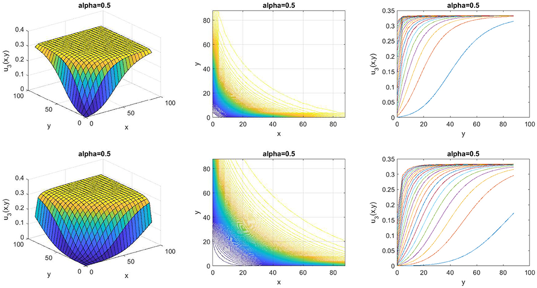
Figure 3. Kink wave solution of Equation (36) in 3D, contour and 2D for Case I.

FIGURE 4

Figure 4. Kink wave solution of Equation (37) in 3D, contour, and 2D for Case II.

4. Solutions Comparison

In this section, the analytical solutions of the non-linear space-time fractional EMC equation and the non-linear space-time fractional AKNS equation obtained by the SE method can be expressed in a simpler form than the G′/G-expansion method [25] as in Tables 1, 2.

TABLE 1

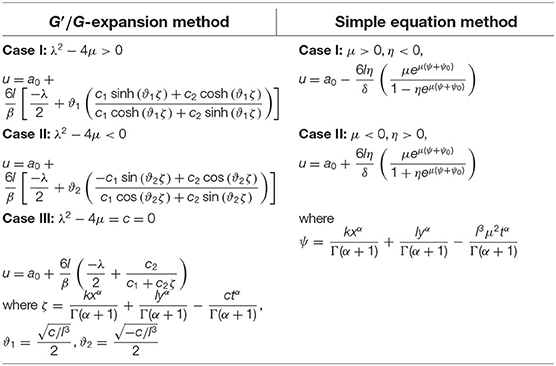
Table 1. Solutions comparison of the non-linear space-time frational Estevez-Mansfield-Clarkson (EMC) equation between G′/G-expansion method and simple equation (SE) method.

TABLE 2

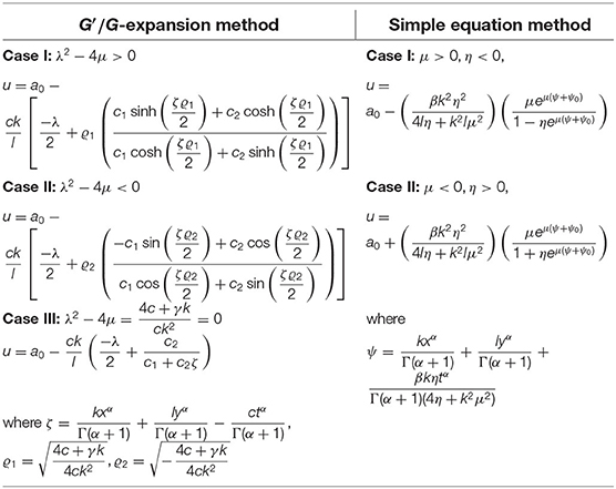
Table 2. Solutions comparison of the non-linear space-time fractional Ablowitz-Kaup-Newell-Segur (AKNS) equation between G′/G-expansion method and simple equation (SE) method.

5. Conclusion

In this study, we solved some fractional shallow water equations and fractional optical fiber equations which are the non-linear space-time fractional EMC equation and the non-linear space-time fractional AKNS equation, respectively. We converted these equations to nODEs by Jumarie's Riemann-Liouville derivative and defined the solutions by an efficient method, the SE method with the Bernoulli equation. The new analytical solutions of the non-linear space-time fractional EMC equation are presented in 2 cases of the exponential solutions as shown in Equations (25)-(26). After we set some parameters, the wave effects of this equation were kink waves as displayed in Figures 1, 2. The 2 cases of the new analytical solutions of the non-linear space-time fractional AKNS equation were exponential solutions as appeared in Equations (36)-(37). The kink wave effects of this equation are displayed in Figures 3, 4. Tables 1, 2 showed our solutions have a simpler form compared to the solution obtained by the G′/G-expansion method [25].

Data Availability Statement

The original contributions presented in the study are included in the article/supplementary material, further inquiries can be directed to the corresponding author.

Author Contributions

Both authors listed have made a substantial, direct, and intellectual contribution to the work and approved it for publication.

Conflict of Interest

The authors declare that the research was conducted in the absence of any commercial or financial relationships that could be construed as a potential conflict of interest.

Publisher's Note

All claims expressed in this article are solely those of the authors and do not necessarily represent those of their affiliated organizations, or those of the publisher, the editors and the reviewers. Any product that may be evaluated in this article, or claim that may be made by its manufacturer, is not guaranteed or endorsed by the publisher.

References

1. Arqub OA, Shawagfeh N. Application of reproducing kernel algorithm for solving Dirichlet time-fractional diffusion-Gordon types equations in porous media. J Porous Media. (2019) 22:411–34. doi: 10.1615/JPorMedia.2019028970

CrossRef Full Text | Google Scholar

2. Momani S, Maayah B, Arqub OA. The reproducing kernel algorithm for numerical solution of Van der Pol damping model in view of the Atangana-Baleanu fractional approach. Fractals. (2020) 28:2040010. doi: 10.1142/S0218348X20400101

CrossRef Full Text | Google Scholar

3. Appadu AR, Tijani YO. 1D Generalised Burgers-Huxley: proposed solutions revisited and numerical solution using FTCS and NSFD methods. Front Appl Math Stat. (2022) 7:773733. doi: 10.3389/fams.2021.773733

CrossRef Full Text | Google Scholar

4. Demiray ST, Pandir Y, Bulut H. Generalized Kudryashov method for time-fractional differential equations. Abstract Appl Anal. (2014) 2014:1–13. doi: 10.1155/2014/901540

CrossRef Full Text | Google Scholar

5. Gaber AA, Aljohani AF, Ebaid A, Machado JT. The generalized Kudryashov method for nonlinear space-time fractional partial differential equations of Burgers type. Nonlinear Dyn. (2019) 95:361–8. doi: 10.1007/s11071-018-4568-4

CrossRef Full Text | Google Scholar

6. Ege SM, Misirli E. Extended Kudryashov method for fractional nonlinear differential equations. Math Sci Appl e-Notes. (2018) 6:19–28. doi: 10.36753/mathenot.421751

CrossRef Full Text | Google Scholar

7. Ege SM, Misirli E. The modified Kudryashov method for solving some fractional-order nonlinear equations. Adv Diff Equat. (2014) 2014:135. doi: 10.1186/1687-1847-2014-135

CrossRef Full Text | Google Scholar

8. Kumar D, Seadawy AR, Joardar AK. Modified Kudryashov method via new exact solutions for some conformable fractional differential equations arising in mathematical biology. Chin J Phys. (2018) 56:75–85. doi: 10.1016/j.cjph.2017.11.020

CrossRef Full Text | Google Scholar

9. Eslami M, Vajargah BF, Mirzazadeh M, Biswas A. Application of first integral method to fractional partial differential equations. Indian J Phys. (2014) 88:177–84. doi: 10.1007/s12648-013-0401-6

CrossRef Full Text | Google Scholar

10. Ilie M, Biazar J, Ayati Z. The first integral method for solving some conformable fractional differential equations. Optical Quant Electron. (2018) 50:55. doi: 10.1007/s11082-017-1307-x

CrossRef Full Text | Google Scholar

11. Lu B. The first integral method for some time fractional differential equations. J Math Anal Appl. (2012) 395:684–93. doi: 10.1016/j.jmaa.2012.05.066

CrossRef Full Text | Google Scholar

12. Bekir A, G!!!. Exact solutions of nonlinear fractional differential equations by G′/G-expansion method. Chin Phys B. (2013) 22:110202. doi: 10.1088/1674-1056/22/11/110202

CrossRef Full Text | Google Scholar

13. Bekir A, G!!!. The G′/G-expansion method using modified Riemann-Liouville derivative for some space-time fractional differential equations. Ain Shams Eng J. (2014) 5:959–65. doi: 10.1016/j.asej.2014.03.006

CrossRef Full Text | Google Scholar

14. Baishya C, Rangarajan R. A new application of G′/G-expansion method for travelling wave solutions of fractional PDEs. Int J Appl Eng Res. (2018) 13:9936–42. doi: 10.37622/000000

CrossRef Full Text | Google Scholar

15. Alzaidy JF. Fractional sub-equation method and its applications to the space-time fractional differential equations in mathematical physics. Brit J Math Comput Sci. (2013) 3:153–63. doi: 10.9734/BJMCS/2013/2908

CrossRef Full Text | Google Scholar

16. Mohyud-Din ST, Nawaz T, Azhar E, Akbar MA. Fractional sub-equation method to space-time fractional Calogero-Degasperis and potential Kadomtsev-Petviashvili equations. J Taibah Univers Sci. (2017) 11:258–63. doi: 10.1016/j.jtusci.2014.11.010

CrossRef Full Text | Google Scholar

17. Zhang S, Zhang H. Fractional sub-equation method and its applications to nonlinear fractional PDEs. Phys Lett A. (2011) 375:1069–73. doi: 10.1016/j.physleta.2011.01.029

CrossRef Full Text | Google Scholar

18. Bhatti MM, Lu DQ. Analytical study of the head-on collision process between hydroelastic solitary waves in the presence of a uniform current. Symmetry. (2019) 11:333. doi: 10.3390/sym11030333

CrossRef Full Text | Google Scholar

19. Bhatti MM, Lu DQ. An application of Nwogu's Boussinesq model to analyze the head-on collision process between hydroelastic solitary waves. Open Phys. (2019) 17:177–91. doi: 10.1515/phys-2019-0018

CrossRef Full Text | Google Scholar

20. Jumarie G. Modified Riemann-Liouville derivative and fractional Taylor series of non-differentiable functions further results. Comput Math Appl. (2006) 51:1367–76. doi: 10.1016/j.camwa.2006.02.001

CrossRef Full Text | Google Scholar

21. Jumarie G. Table of some basic fractional calculus formulae derived from a modified Riemann-Liouville derivative for non-differentiable functions. Appl Math Lett. (2009) 22:378–85. doi: 10.1016/j.aml.2008.06.003

CrossRef Full Text | Google Scholar

22. Mansfield EL, Clarkson PA. Symmetries and exact solutions for a 2+1-dimensional shallow water wave equation. Math Comput Simul. (1997) 43:39–55. doi: 10.1016/S0378-4754(96)00054-7

CrossRef Full Text | Google Scholar

23. Zhen-Ya Y. Abundant symmetries and exact compacton-like structures in the two-parameter family of the Estevez Mansfield Clarkson equations. Commun Theoret Phys. (2002) 37:27–34. doi: 10.1088/0253-6102/37/1/27

CrossRef Full Text | Google Scholar

24. Asghar A, Seadawy AR, Dianchen L. Computational methods and traveling wave solutions for the fourth-order nonlinear Ablowitz-Kaup-Newell-Segur water wave dynamical equation via two methods and its applications. Open Phys. (2018) 16:219–26. doi: 10.1515/phys-2018-0032

CrossRef Full Text | Google Scholar

25. Phoosree S, Chinviriyasit S. New analytic solutions of some fourth-order nonlinear space-time fractional partial differential equations by G′/G-expansion method. Songklanakarin J Sci Technol. (2021) 43:795–801. doi: 10.14456/sjst-psu.2021.105

CrossRef Full Text | Google Scholar

26. Nofal TA. Simple equation method for nonlinear partial differential equations and its applications. J Egypt Math Soc. (2016) 24:204–9. doi: 10.1016/j.joems.2015.05.006

PubMed Abstract | CrossRef Full Text | Google Scholar

27. Phoosree S. (2019). Exact solutions for the Estevez-Mansfield-Clarkson equation (dissertation). King Mongkut's University of Technology Thonburi, Bangkok, Thailand.

Google Scholar

28. Fan E. Extended tanh-function method and its applications to nonlinear equations. Phys Lett A. (2000) 227:212–8. doi: 10.1016/S0375-9601(00)00725-8

CrossRef Full Text | Google Scholar