On the Dynamics of Sexually Transmitted Diseases Under Awareness and Treatment

In this paper, we develop and extend the work of Jia and Qin on sexually transmitted disease models with a novel class of non-linear incidence. Awareness plays a central role both in the susceptible and the infectious classes. The Existence, uniqueness, boundedness, and positivity of solutions are systematically established. Concavity arguments and the occurrence of a vertical asymptote are essential in the proof of the existence of a unique endemic equilibrium. Conditions for the stability of all steady states are investigated. In particular, numerical simulations are performed in order to capture the asymptotic behavior of solutions.

AMS Classification: 92D30, 34D23.

1. Introduction

Disease incidence plays a crucial role in mathematical epidemiology and it is essential in the computation of the basic reproduction number. Non-linear incidences are known to induce complex or chaotic behavior as oppose to standard incidences frequently used in classical infectious disease models [1–6]. A class of non-linear incidences particularly useful in the modeling of sexually transmitted diseases was introduced in [7] by the authors in the modeling of HIV/AIDS epidemic. The model considered however was not properly conceptualized as the density of individuals with full-blown AIDS not receiving ARV treatment did not bear any influence on the infection rate of the disease. In addition a number of inaccuracies are displayed in this paper like the unknown variable T missing in the third equation of system (2.1) and also a mistake occurred in the computation of the sign of a₃ in the proof of the stability of the endemic equilibrium. The purpose of this paper is to develop and extend the work on [7] by deriving a realistic model for sexually transmitted diseases with a proper non-linear incidence rate with a valid biological significance and perform a full analysis of the resulting model. In Section 2, the model is derived and presented. Well-posedness analysis, positivity and boundedness are considered in Section 3 followed by stability analysis of the critical points of the system in Section 4, numerical simulations in Section 5 and the conclusion.

2. The Model

In this paper, a model with five compartments is formulated with non-linear incidence Sg(t, I) incorporated into it. The incidence is presumed to be a time dependent non-linear response to the size of the infectious population.

The compartments are denoted by S(t), I(t), T(t), A(t) and R(t) which represent the number of susceptible individuals, the number of infected individuals with the potential of transmitting the disease as they are not under treatment and do not take any form of protection while engaging in sexual activities, the number of individuals under treatment, the number of infectious individuals engaging in safe sex, and heathy individuals that engage in safe sex, respectively, at time t. The model represented in Figure 1 is governed by the system of nonlinear ordinary differential equations

$\begin{array}{ll}\{\begin{array}{c}\frac{dS}{dt}=\Gamma -Sg(t,I)-({\omega }_1+d)S,\\ \\ \frac{dI}{dt}=Sg(t,I)+{\nu }_{1}T-(d+{\tau }_1+{\tau }_2)I,\\ \\ \frac{dT}{dt}={\tau }_{2}I-{\nu }_{2}T-(d+{\nu }_1)T,\\ \\ \frac{dA}{dt}={\tau }_{1}I-dA+{\nu }_{2}T,\\ \\ \frac{dR}{dt}={\omega }_{1}S-dR,\end{array}& (1)\end{array}$

endowed with initial conditions

S(0) ≡ S₀ > 0, I(0) ≡ I₀ > 0, T(0) ≡ T₀ ≥ 0, A(0) ≡ A₀ ≥ 0, R(0) ≡ R₀ ≥ 0.

FIGURE 1

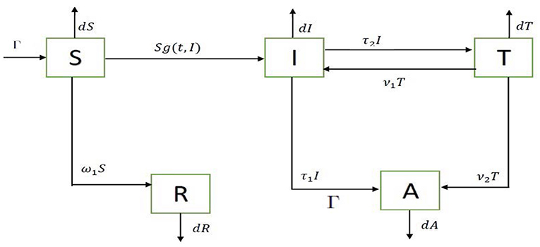
Figure 1. Flow diagram.

The parameters in the evolution system (1) are described in Table 1:

The total population N(t) is given by S(t) + I(t) + T(t) + A(t) + R(t). By adding all the equations of the system (1), we obtain the rate of change of N(t), which is given by

$\begin{array}{ll}\frac{dN}{dt}=\Gamma -dN& (2)\end{array}$

and N(t) varies over time and is nearing a stable fixed point $\frac{\Gamma }{d}$ as t → ∞. Therefore, the biologically feasible region for the system (1) is given by

$\begin{array}{l}\Psi =\{(S,I,T,A,R)\in {ℝ}_{+}^5|0<S(t)+I(t)+T(t)+A(t)+R(t)\le \frac{\Gamma }{d}\}.\end{array}$

It is easy to see that the set Ψ is positively invariant. Next we present a systematic analysis of our evolution equation.

TABLE 1

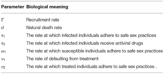
Table 1. Biological meaning of parameters.

3. Mathematical Analysis

We start by investigating the well-posedness of the model (1). Given the fact that the variables represent biologically densities, it is important to show that all the variables remain positive at all time.

Lemma 1. For any non-negative initial conditions (S₀, I₀, T₀, A₀, R₀), system (1) has a local solution which is unique.

Proof: Let x = (S, I, T, A, R), system (1) can be rewritten as x′(t) = f(t, x(t)), where f : ℝ⁶ → ℝ⁵ is a C¹ vector field. By the classical differential equation theory, we can confirm that system (1) has a unique local solution defined in a maximum interval [0, t_m).□

Lemma 2. For any non-negative initial conditions (S₀, I₀, T₀, A₀, R₀), the solution of (1) is non-negative and bounded for all t ∈ [0, t_m).

Proof: We start by showing positivity of the local solution for any non-negative initial conditions. It is easy to see that S(t) ≥ 0 for all t ∈ [0, t_m). Indeed, assume the contrary and let t₁ > 0 be the first time such that S(t₁) = 0 and $S^{\prime }(t_1)<0$. From the first equation of the system (1), we have $S^{\prime }(t_1)=\Gamma >0$, which presents a contradiction. Therefore S(t) ≥ 0 for all t ∈ [0, t_m). Using the same argument, positivity I(t), T(t), A(t) and R(t) in the interval [0, t_m) are established. Furthermore from (2), we have that

$\begin{array}{ll}N(t)=\frac{\Gamma }{d}+N(0)e^{-dt}\le \frac{\Gamma }{d}+N(0).& (3)\end{array}$

Therefore the solution N(t) is bounded in the interval [0, t_m).□

Theorem 1 For any non-negative initial conditions (S₀, I₀, T₀, A₀, R₀), system (1) has a unique global solution. Moreover, this solution is non-negative and bounded for all t ≥ 0.

Proof: The solution does not blow up in a finite time as it is bounded, it is therefore defined at all time t ≥ 0. Other properties of the solution follow from lemma (1) and lemma (2).□

Setting m = d + τ₁ + τ₂ and n = d + ν₁ + ν₂, system (1) transforms into a reduced system

$\begin{array}{ll}\{\begin{array}{c}\frac{dS}{dt}=\Gamma -Sg(t,I)-({\omega }_1+d)S,\\ \\ \frac{dI}{dt}=Sg(t,I)+{\nu }_{1}T-mI,\\ \\ \frac{dT}{dt}={\tau }_{2}I-nT,\\ \\ \frac{dA}{dt}={\tau }_{1}I-dA+{\nu }_{2}T,\\ \\ \frac{dR}{dt}={\omega }_{1}S-dR.\end{array}& (4)\end{array}$

4. Models With Time Independent Non-linear Response

In this section, we assume that the non-linear response function is not time dependent, ie g(t, I) ≡ g(I). Following [7], it is further assumed that

$\begin{array}{l}({\text{H}}_1):g(0)=0,g^{\prime }(0)>0,g^{″}(I)\le 0\text{ for }I\ge 0,\\ ({\text{H}}_2):{\displaystyle \underset{I\to 0^{+}}{lim}}\frac{g(I)}{I}=k,0<k<\infty .\end{array}$

4.1. The Basic Reproduction Number

In this section, we use the next generation method [8] to obtain the basic reproduction number. Let z be the transpose of (I, A, T, S, R). We rewrite the system (4) in the matrix form

$\begin{array}{l}\frac{dz}{dt}={F}(z)-{V}(z),\end{array}$

where

$\begin{array}{l}{F}(z)=\left(\begin{array}{c}Sg(I)\\ 0\\ 0\\ 0\\ 0\end{array}\right)\end{array}$

and

$\begin{array}{l}{V}(z)=\left(\begin{array}{c}mI-{\nu }_{1}T\\ dA-{\tau }_{1}I-{\nu }_{2}T\\ nT-{\tau }_{2}I\\ Sg(I)+({\omega }_1+d)S-\Gamma \\ dR-{\omega }_{1}S\end{array}\right).\end{array}$

The disease free equilibrium of system (4) takes the form

$E^0=(I^0,A^0,T^0,S^0,R^0)=\left(0,0,0,\frac{\Gamma }{{\omega }_1+d},\frac{{\omega }_1\Gamma }{d({\omega }_1+d)}\right).$

Following [8], we compute the basic reproduction number using the formula below

${{R}}_0=\rho (F{V}^{-1}),$

where

$F=\left[\begin{array}{ccc}\frac{\partial {{F}}_1}{\partial E}& \frac{\partial {{F}}_1}{\partial I}& \frac{\partial {{F}}_1}{\partial T}\\ & & \\ 0& 0& 0\\ 0& 0& 0\end{array}\right]{|}_{(E^0,I^0,T^0,S^0,R^0)}=\left[\begin{array}{ccc}\frac{\alpha \Gamma }{{\omega }_1+d}& 0& 0\\ 0& 0& 0\\ 0& 0& 0\end{array}\right]$

and

$V=\left[\begin{array}{lll}\frac{\partial {{V}}_1}{\partial E}\hfill & \frac{\partial {{V}}_1}{\partial I}\hfill & \frac{\partial {{V}}_1}{\partial T}\hfill \\ \frac{\partial {{V}}_2}{\partial E}\hfill & \frac{\partial {{V}}_2}{\partial I}\hfill & \frac{\partial {{V}}_2}{\partial T}\hfill \\ \frac{\partial {{V}}_3}{\partial E}\hfill & \frac{\partial {{V}}_3}{\partial I}\hfill & \frac{\partial {{V}}_3}{\partial T}\hfill \end{array}\right]{|}_{(E^0,I^0,T^0,S^0,R^0)}\left[\begin{array}{ccc}m& 0& -{\nu }_1\\ -{\tau }_1& d& -{\nu }_2\\ -{\tau }_2& 0& n\end{array}\right]$

and ρ is the spectral radius of the matrix FV⁻¹. Given the fact that

$\begin{array}{l}{V}^{-1}=\frac{1}{d(mn-{\nu }_1{\tau }_2)}\left[\begin{array}{ccc}nd& 0& -{\nu }_{1}d\\ \\ {\tau }_{1}n-{\nu }_2{\tau }_2& mn-{\nu }_1{\tau }_2& {\nu }_{2}m-{\nu }_1{\tau }_1\\ \\ {\tau }_{2}d& 0& md\\ \\ \end{array}\right],\end{array}$

it follows that

$\begin{array}{ll}{{R}}_0=\frac{\alpha n\Gamma }{({\omega }_1+d)(mn-{\nu }_1{\tau }_2)}.& (5)\end{array}$

4.1.1. Stability of the Disease-Free Equilibrium

The stability of the disease-free equilibrium will be investigated in this subsection.

Theorem 2 The disease free equilibrium E⁰ is globally asymptotically stable if $0<{{R}}_0<1$, and unstable if ${{R}}_0>1$.

Proof: The Jacobian matrix $(J_{E^0})$, evaluated at E⁰, is given by

$\begin{array}{ll}{J}_{E^0}=\left(\begin{array}{ccccc}-({\omega }_1+d)& \frac{-\alpha \Gamma }{{\omega }_1+d}& 0& 0& 0\\ \\ 0& \frac{\alpha \Gamma }{{\omega }_1+d}-m& {\nu }_1& 0& 0\\ \\ 0& {\tau }_2& -n& 0& 0\\ \\ 0& {\tau }_1& {\nu }_2& -d& 0\\ \\ {\omega }_1& 0& 0& 0& -d\\ \\ \end{array}\right).& (6)\end{array}$

The characteristic equation that results from the Jacobian matrix $(J_{E^0})$ is given by det$(J_{E^0}-\lambda I)$ = 0. Thus, we get

$\begin{array}{ll}{(d+\lambda )}^2\left[({\omega }_1+d)+\lambda \right]\left[\left(m-\frac{\alpha \Gamma }{{\omega }_1+d}+\lambda \right)(n+\lambda )-{\nu }_1{\tau }_2\right]=0.& (7)\end{array}$

The characteristic equation (7) has three negative real roots, which are

$\begin{array}{l}{\lambda }_1=-d,\\ {\lambda }_2={\lambda }_3=-({\omega }_1+d),\end{array}$

and the other 2 roots, λ₄ and λ₅, are roots of the equation

$\begin{array}{ll}f(\lambda )=\left[\left(m-\frac{\alpha \Gamma }{{\omega }_1+d}\right)+\lambda \right](n+\lambda )-{\nu }_1{\tau }_2\equiv {\lambda }^2+a_1\lambda +a_2=0,& (8)\end{array}$

where

$\begin{array}{l}{a}_1=m+n-\frac{\alpha \Gamma }{{\omega }_1+d},\\ a_2=mn-{\nu }_1{\tau }_2-\frac{\alpha n\Gamma }{{\omega }_1+d}.\end{array}$

We now need to consider the signs of λ₄ and λ₅. Note that

$mn-{\nu }_1{\tau }_2>0.$

Assuming

${{R}}_0=\frac{\alpha n\Gamma }{({\omega }_1+d)(mn-{\nu }_1{\tau }_2)}<1,$

we have that

$mn-{\nu }_1{\tau }_2-\frac{\alpha n\Gamma }{{\omega }_1+d}=a_2>0.$

Moreover

$\frac{\alpha n\Gamma }{{\omega }_1+d}<mn-{\nu }_1{\tau }_2<mn.$

It implies that

$m-\frac{\alpha \Gamma }{{\omega }_1+d}>0.$

It follows that a₁ > 0. As a result the roots λ₄ and λ₅ are strictly negative. We can conclude that all roots of (7) have negative real parts, therefore, the disease free equilibrium is locally asymptotically stable [8–10]. Furthermore assuming that

${{R}}_0=\frac{\alpha n\Gamma }{({\omega }_1+d)(mn-{\nu }_1{\tau }_2)}>1,$

we have that a₂ < 0, it follows that the characteristic equation f(λ) = 0 has a least a strictly positive root. Therefore, the disease free equilibrium E⁰ is unstable.

4.2. Existence of an Endemic Equilibrium

In this subsection, we investigate the existence of an endemic equilibrium for the system (4).

Proposition 1. The system of differential equations (4) admits a unique endemic equilibrium if and only if ${{R}}_0>1$.

Proof: Let E^* = (S^*, I^*, T^*, A^*, R^*) be an equilibrium point. Then the components of E^* satisfy the following set of equations

$\begin{array}{ll}\{\begin{array}{cc}\Gamma -S^{*}g(I^{*})-({\omega }_1+d)S^{*}& =0,\\ \\ S^{*}g(I^{*})+{\nu }_1{T}^{*}-m{I}^{*}& =0,\\ \\ {\tau }_2{I}^{*}-n{T}^{*}& =0,\\ \\ {\tau }_1{I}^{*}-d{A}^{*}+{\nu }_2{T}^{*}& =0,\\ \\ {\omega }_1{S}^{*}-d{R}^{*}& =0.\end{array}& (9)\end{array}$

From the last three equations of the system (9), we have that

$\begin{array}{l}{T}^{*}=\frac{{\tau }_2{I}^{*}}{n},\\ A^{*}=\frac{{\tau }_1+\frac{{\nu }_2{\tau }_2}{n}}{d}{I}^{*},\\ R^{*}=\frac{{\omega }_1{S}^{*}}{d}.\end{array}$

Substituting T^*, A^* and R^* into the first two equations, we obtain

$\begin{array}{l}\Gamma -S^{*}g(I^{*})-({\omega }_1+d)S^{*}=0,\\ S^{*}g(I^{*})-\left(\frac{{\nu }_1{\tau }_2}{n}-m\right)I^{*}=0.\end{array}$

It follows that

$\begin{array}{ll}{S}^{*}=\frac{\left(m-\frac{{\nu }_1{\tau }_2}{n}\right)I^{*}}{g(I^{*})}& (10)\end{array}$

and

$\begin{array}{ll}\Gamma -\left(m-\frac{{\nu }_1{\tau }_2}{n}\right)I^{*}-({\omega }_1+d)\frac{\left(m-\frac{{\nu }_1{\tau }_2}{n}\right)I^{*}}{g(I^{*})}=0.& (11)\end{array}$

Next we set

$\begin{array}{ll}h(I):=\frac{({\omega }_1+d)\left(m-\frac{{\nu }_1{\tau }_2}{n}\right)I}{\Gamma -\left(m-\frac{{\nu }_1{\tau }_2}{n}\right)I}.& (12)\end{array}$

It is enough to show that there exists a point I^* ∈ ℝ⁺ such that h(I^*) = g(I^*). In other words, we will show that the curves of the functions h and g intersect at a point I^*.

Note that

$I=\frac{n\Gamma }{mn-{\nu }_1{\tau }_2}$

is a vertical asymptote of the function h(I). For all

$0<I<\frac{n\Gamma }{mn-{\nu }_1{\tau }_2},$

we have that

$\begin{array}{l}{h}^{\prime }(I)=\\ \frac{\left({\omega }_1+d\right)\left(m-\frac{{\nu }_1{\tau }_2}{n}\right)\left[\Gamma -\left(m-\frac{{\nu }_1{\tau }_2}{n}\right)I\right]+\left({\omega }_1+d\right){\left(m-\frac{{\nu }_1{\tau }_2}{n}\right)}^{2}I}{{\left[\Gamma -\left(m-\frac{{\nu }_1{\tau }_2}{n}\right)I\right]}^2}\\ =\frac{\Gamma \left({\omega }_1+d\right)\left(m-\frac{{\nu }_1{\tau }_2}{n}\right)}{{\left[\Gamma -\left(m-\frac{{\nu }_1{\tau }_2}{n}\right)I\right]}^2}>0\end{array}$

and

$\begin{array}{l}{h}^{″}(I)=\frac{2\left[\Gamma -\left(m-\frac{{\nu }_1{\tau }_2}{n}\right)I\right]{\left(m-\frac{{\nu }_1{\tau }_2}{n}\right)}^2\Gamma \left({\omega }_1+d\right)}{{\left[\Gamma -\left(m-\frac{{\nu }_1{\tau }_2}{n}\right)I\right]}^4}\\ =\frac{2\Gamma \left({\omega }_1+d\right){\left(m-\frac{{\nu }_1{\tau }_2}{n}\right)}^2}{{\left[\Gamma -\left(m-\frac{{\nu }_1{\tau }_2}{n}\right)I\right]}^3}>0.\end{array}$

It follows that the function h is increasing and concave upward in the interval

$\left[0,\frac{n\Gamma }{mn-{\nu }_1{\tau }_2}\right)$

with a vertical asymptote at the right end of the interval. Note that the function g is increasing and concave downward in the closed interval

$\left[0,\frac{n\Gamma }{mn-{\nu }_1{\tau }_2}\right].$

As a result if

$g^{\prime }(0)>h^{\prime }(0)=\frac{({\omega }_1+d)\left(m-\frac{{\nu }_1{\tau }_2}{n}\right)}{\Gamma },$

which is equivalent to the condition ${{R}}_0>1$, then Equation (12) has a unique root I^* in the interval

$\left(0,\frac{n\Gamma }{mn-{\nu }_1{\tau }_2}\right).$

Furthermore if

$I>\frac{n\Gamma }{mn-{\nu }_1{\tau }_2},$

then h(I) < 0. There is no intersection point with g(I) since g is a positive function. Therefore there exists a unique endemic equilibrium point E^* = (S^*, I^*, T^*, A^*, R^*) provided that ${{R}}_0>1$. In addition if

$g^{\prime }(0)\ge h^{\prime }(0)=\frac{({\omega }_1+d)\left(m-\frac{{\nu }_1{\tau }_2}{n}\right)}{\Gamma },$

equivalent to the condition ${{R}}_0\le 1$, there is no endemic equilibrium for the system (4).

4.2.1. Stability of the Endemic Equilibrium

Lemma 3. Let g(I) be a positive smooth function defined on the interval [0, ∞). Suppose that assumptions H₁ and H₂ hold, then the following inequality is satisfied

$\begin{array}{ll}1-\frac{I{g}^{\prime }(I)}{g(I)}\ge 0foranyI>0.& (13)\end{array}$

Proof:

We have that

$\begin{array}{l}\frac{d\left[g(I)-I{g}^{\prime }(I)\right]}{dI}=-I{g}^{″}(I)\ge 0\end{array}$

as g″(I) ≤ 0. This implies that the function g(I) − Ig′(I) is increasing on the interval [0, ∞). Given the fact that g(0) − 0g′(0) = 0, it follows that g(I) − Ig′(I) ≥ 0.□

Theorem 3 If ${{R}}_0>1$, then the endemic equilibrium E^* is locally asymptotically stable.

Proof: The Jacobian matrix of the endemic equilibrium is given by

$\begin{array}{ll}{J}_{E^{*}}=\left(\begin{array}{ccccc}-g(I^{*})-({\omega }_1+d)& S^{*}{g}^{\prime }(I^{*})& 0& 0& 0\\ \\ g(I^{*})& S^{*}{g}^{\prime }(I^{*})-m& {\nu }_1& 0& 0\\ \\ 0& {\tau }_2& -n& 0& 0\\ \\ 0& {\tau }_1& {\nu }_2& -d& 0\\ \\ {\omega }_1& 0& 0& 0& -d\\ \\ \end{array}\right).& (14)\end{array}$

The characteristic equation that results from the Jacobian matrix $(J_{E^{*}})$ is given by det$(J_{E^{*}}-\lambda I)$ = 0. Thus, we get

$\begin{array}{ll}{(d+\lambda )}^2({\lambda }^3+b_1{\lambda }^2+b_2\lambda +b_3)=0,& (15)\end{array}$

where

$\begin{array}{l}{b}_1=g(I^{*})+{\omega }_1+d+m+n-S^{*}{g}^{\prime }(I^{*}),\\ b_2=(m+n)\left[g(I^{*})+{\omega }_1+d\right]-S^{*}{g}^{\prime }(I^{*})({\omega }_1+d+n)+mn-{\nu }_1{\tau }_2,\\ b_3=(mn-{\nu }_1{\tau }_2)\left[g(I^{*})+{\omega }_1+d\right]-n({\omega }_1+d)S^{*}{g}^{\prime }(I^{*}).\end{array}$

The characteristic Equation (15) has a negative real double root

$\begin{array}{l}{\lambda }_1={\lambda }_2=-d,\end{array}$

and three other roots, λ₃, λ₄ and λ₅, which are the roots of the equation

$\begin{array}{ll}{\lambda }^3+b_1{\lambda }^2+b_2\lambda +b_3=0.& (16)\end{array}$

From Lemma (3), we have that

$\begin{array}{ll}1-\frac{I^{*}}{g(I^{*})}{g}^{\prime }(I^{*})\ge 0.& (17)\end{array}$

It follows that

$\begin{array}{l}m-S^{*}{g}^{\prime }(I^{*})=m-\frac{\left(m-\frac{{\nu }_1{\tau }_2}{n}\right)I^{*}}{g(I^{*})}{g}^{\prime }(I^{*})\\ >m\left[1-\frac{I^{*}}{g(I^{*})}{g}^{\prime }(I^{*})\right]\ge 0.& (18)\end{array}$

Hence,

$\begin{array}{l}{b}_1=g(I^{*})+{\omega }_1+d+m+n-S^{*}{g}^{\prime }(I^{*})>0\text{ using }18,\\ b_2=(m+n)\left[g(I^{*})+{\omega }_1+d\right]-S^{*}{g}^{\prime }(I^{*})({\omega }_1+d+n)+mn-{\nu }_1{\tau }_2\\ =(m+n)g(I^{*})+({\omega }_1+d)\left[m+n-S^{*}{g}^{\prime }(I^{*})\right]-n{S}^{*}{g}^{\prime }(I^{*})+\\ mn-{\nu }_1{\tau }_2\\ =(m+n)g(I^{*})+({\omega }_1+d)\left[m+n-S^{*}{g}^{\prime }(I^{*})\right]+\\ n\left[m-\frac{\left(m-\frac{{\nu }_1{\tau }_2}{n}\right)I^{*}}{g(I^{*})}{g}^{\prime }(I^{*})\right]-{\nu }_1{\tau }_2\\ =(m+n)g(I^{*})+({\omega }_1+d)\left[m+n-S^{*}{g}^{\prime }(I^{*})\right]+\\ (mn-{\nu }_1{\tau }_2)\left[1-\frac{I^{*}}{g(I^{*})}{g}^{\prime }(I^{*})\right]>0\text{ using }17,\end{array}$

and

$\begin{array}{l}{b}_3=(mn-{\nu }_1{\tau }_2)\left[g(I^{*})+{\omega }_1+d\right]-n({\omega }_1+d)S^{*}{g}^{\prime }(I^{*})\\ =(mn-{\nu }_1{\tau }_2)\left[g(I^{*})+{\omega }_1+d\right]\\ -({\omega }_1+d)\left[\frac{(mn-{\nu }_1{\tau }_2)I^{*}}{g(I^{*})}{g}^{\prime }(I^{*})\right]\\ =(mn-{\nu }_1{\tau }_2)\left[g(I^{*})+{\omega }_1+d-({\omega }_1+d)\frac{I^{*}}{g(I^{*})}{g}^{\prime }(I^{*})\right]\\ =(mn-{\nu }_1{\tau }_2)\{g(I^{*})+({\omega }_1+d)\left[1-\frac{I^{*}}{g(I^{*})}{g}^{\prime }(I^{*})\right]\}>0\\ \text{using }17.\end{array}$

Moreover we have that

$\begin{array}{l}{b}_1{b}_2-b_3\\ =b_1\{(m+n)g(I^{*})+({\omega }_1+d)\left[m+n-S^{*}{g}^{\prime }(I^{*})\right]\}\\ -(mn-{\nu }_1{\tau }_2)g(I^{*})\\ +b_1\left\{(mn-{\nu }_1{\tau }_2)\left(1-\frac{I^{*}}{g(I^{*})}{g}^{\prime }(I^{*})\right)\right\}\\ -\left\{(mn-{\nu }_1{\tau }_2)\left[({\omega }_1+d)\left(1-\frac{I^{*}}{g(I^{*})}{g}^{\prime }(I^{*})\right)\right]\right\}.\end{array}$

It follows that

$\begin{array}{l}{b}_1{b}_2-b_3\\ >n\{(m+n)g(I^{*})+({\omega }_1+d)\left[m+n-S^{*}{g}^{\prime }(I^{*})\right]\}-mng(I^{*})+\\ \left\{(mn-{\nu }_1{\tau }_2)\left[({\omega }_1+d)\left(1-\frac{I^{*}}{g(I^{*})}{g}^{\prime }(I^{*})\right)\right]\left[g(I^{*})+m-S^{*}{g}^{\prime }(I^{*})\right]\right\}\\ >0.\end{array}$

As a result, by the Routh−Hurwitz stability criterion [11], all the roots of the characteristic polynomial (15) have strictly negative real parts. Therefore the endemic equilibrium is locally asymptotically stable.

5. Numerical Simulations

In this section, we provide numerical simulations for the evolution system of ordinary differential equations (1) to support the theoretical findings. Without loss of generality we set

$g(I)=\frac{\alpha (t)I}{1+\beta (t)I}.$

Note that conditions of assumptions (H₁) and (H₂) are satisfied. Furthermore we let

$\begin{array}{l}\Gamma =150,{\omega }_1=1,d=2,{\nu }_1=1,\\ {\nu }_2=1,{\tau }_1=2,{\tau }_2=3.\end{array}$

Next we explore two scenarios involving static simulations and time-dependent simulations respectively.

5.1. Static Simulations

Picking $\alpha =\frac{1}{12}$ and β = 1 and substituting in the expression of the basic reproduction number, we get that ${{R}}_0=\frac{2}{3}<1$. According to Theorem 2 the disease-free equilibrium, E⁰ = (50, 0, 0, 0, 25), is globally asymptotically stable. In Figure 2, it clearly shows that the disease eventually dies out.

FIGURE 2

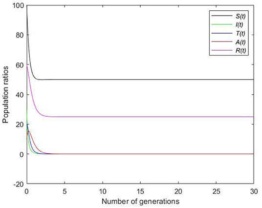
Figure 2. Static simulation for disease-free equilibrium.

Picking $\alpha =\frac{1}{5}$ and β = 0.1 and substituting in the expression of the basic reproduction number, we get that ${{R}}_0=1.6>1$. According to Theorem 3 the endemic equilibrium, E^* = (42.5, 3.6, 2.7, 4.9, 21.2), is locally asymptotically stable. In Figure 3, all the graphs converge to the endemic equilibrium.

FIGURE 3

Figure 3. Static simulation for endemic equilibrium.

5.2. Time-Dependent Simulations

Picking $\alpha (t)=\frac{1}{5+2t}$, it can be observed in Figure 4 that graphs converge to the disease free equilibrium as time increases. It therefore suggests the global asymptotical stability of the disease free equilibrium and the extension of the disease in time.

FIGURE 4

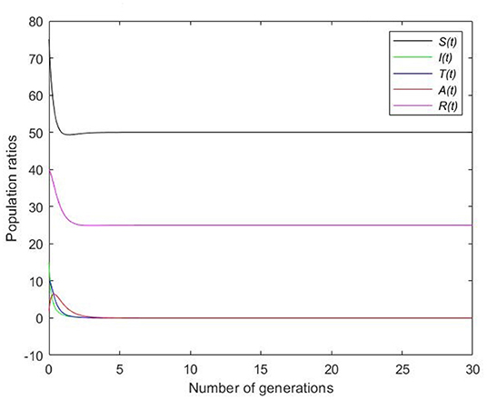
Figure 4. Simulation with time dependence for disease-free equilibrium.

Picking $\alpha (t)=t^2+\frac{5}{4}$, Figure 5 clearly shows that the susceptible population vanishes in a short span of time and the disease essentially affects all people in the population.

FIGURE 5

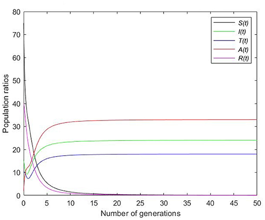
Figure 5. Simulation with time dependence for endemic equilibrium.

6. Concluding Remarks

In this paper, we formulated and investigated a mathematical model describing the dynamics on sexually transmitted disease models with a novel class of non-linear incidence. We showed that the derived non-autonomous system of differential equations governing the evolution of the process was well-posed and the solution happened to be positive and bounded. The role of awareness in the susceptible and infectious classes was explored and investigated. A vertical asymptote and concavity arguments were critical in the proof of existence of an endemic equilibrium for the system and its asymptotical stability. In particular, numerical simulations were performed in order to predict the asymptotic behavior of solutions and support the theoretical findings.

Data Availability Statement

The original contributions presented in the study are included in the article/supplementary material, further inquiries can be directed to the corresponding author/s.

Author Contributions

All authors contributed to all critical aspects of the analysis and simulations. All authors contributed to the article and approved the submitted version.

Conflict of Interest

The authors declare that the research was conducted in the absence of any commercial or financial relationships that could be construed as a potential conflict of interest.

Publisher's Note

All claims expressed in this article are solely those of the authors and do not necessarily represent those of their affiliated organizations, or those of the publisher, the editors and the reviewers. Any product that may be evaluated in this article, or claim that may be made by its manufacturer, is not guaranteed or endorsed by the publisher.

References

1. Mbokoma M, Oukouomi Noutchie SC. A stochastic analysis of HIV dynamics driven by fractional Browanian motion. J Algebra Appl Math. (2017) 15:1–31.

Google Scholar

2. Mbokoma M, Oukouomi Noutchie SC. A theoretical analysis of the dynamics of AIDS with random condom use. J Anal Appl. (2017) 15:85–115.

Google Scholar

3. Marin M, Othman MIA, Abbas IA. An extension of the domain of influence theorem for generalized thermoelasticity of anisotropic material with voids. J Comput Theoret Nanosci. (2015) 12:1594–8. doi: 10.1166/jctn.2015.3934

CrossRef Full Text | Google Scholar

4. Ogunlaran OM, Oukouomi Noutchie SC. Mathematical model for an effective management of HIV infection. Biomed Res Int. (2016) 2016:4217548. doi: 10.1155/2016/4217548

PubMed Abstract | CrossRef Full Text | Google Scholar

5. Othman MIA, Said S, Marin M. A novel model of plane waves of two-temperature fiber-reinforced thermoelastic medium under the effect of gravity with three-phase-lag model. Int J Num Methods Heat Fluid Flow. (2019) 29:4788-806. doi: 10.1108/HFF-04-2019-0359

CrossRef Full Text | Google Scholar

6. Tewa JJ, Bowong S, Oukouomi Noutchie SC. Mathematical analysis of a two-patch model of tuberculosis disease with staged progression. Appl Math Modell. (2012) 36:5792–807. doi: 10.1016/j.apm.2011.09.004

CrossRef Full Text | Google Scholar

7. Jia J, Qin G. Stability analysis of HIV/AIDS epidemic model with nonlinear incidence and treatment. Adv Diff Equat. (2017) 2017:136. doi: 10.1186/s13662-017-1175-5

PubMed Abstract | CrossRef Full Text | Google Scholar

8. Van den Driessche P, Watmough J. Reproduction numbers and sub-threshold endemic equilibria for compartmental models of disease transmission. Math. Biosci. (2002) 180:29–48. doi: 10.1016/S0025-5564(02)00108-6

PubMed Abstract | CrossRef Full Text | Google Scholar

9. Verhulst F. Nonlinear Differential Equations and Dynamical Systems. New York, NY: Springer-Verlag (1990).

PubMed Abstract | Google Scholar

10. LaSalle JP. The Stability of Dynamical Systems. Philadelphia, PA: SIAM (1976).

11. Murray JD. Mathematical Biology I. An Introduction. 3rd ed., New York: Springer-Verlag. (2002).

Google Scholar