Hybrid A* path search with resource constraints and dynamic obstacles

This paper considers path planning with resource constraints and dynamic obstacles for an unmanned aerial vehicle (UAV), modeled as a Dubins agent. Incorporating these complex constraints at the guidance stage expands the scope of operations of UAVs in challenging environments containing path-dependent integral constraints and time-varying obstacles. Path-dependent integral constraints, also known as resource constraints, can occur when the UAV is subject to a hazardous environment that exposes it to cumulative damage over its traversed path. The noise penalty function was selected as the resource constraint for this study, which was modeled as a path integral that exerts a path-dependent load on the UAV, stipulated to not exceed an upper bound. Weather phenomena such as storms, turbulence and ice are modeled as dynamic obstacles. In this paper, ice data from the Aviation Weather Service is employed to create training data sets for learning the dynamics of ice phenomena. Dynamic mode decomposition (DMD) is used to learn and forecast the evolution of ice conditions at flight level. This approach is presented as a computationally scalable means of propagating obstacle dynamics. The reduced order DMD representation of time-varying ice obstacles is integrated with a recently developed backtracking hybrid A∗ graph search algorithm. The backtracking mechanism allows us to determine a feasible path in a computationally scalable manner in the presence of resource constraints. Illustrative numerical results are presented to demonstrate the effectiveness of the proposed path-planning method.

1 Introduction

In recent years, there has been considerable interest in incorporating complex constraints into path-planning for autonomous vehicles so as to expand their scope of operation in challenging environments. This paper considers two forms of complex constraints for path planning of a Dubins agent: 1) time-varying obstacles that are capable of translation, rotation, as well as changing their shape, and 2) resource constraints that exert a path-dependent cumulative load (or damage) on the vehicle that must be maintained under a stipulated threshold. In the context of unmanned aerial vehicles (UAVs), examples of the former include weather phenomena, such as storms, turbulence and ice. In the case of resource constraints, the agent is allowed to “fly through” the obstacle, so long as the total accumulated damage incurred along its path is kept under a stipulated threshold. Examples of such path-dependent loading constraints include flight of a UAV over a wildfire, wherein the resource constraint represents placing an upper limit on the increase in temperature along the agent’s path to keep onboard equipment safe. Other scenarios include flight over an urban region while maintaining the total noise generated along its trajectory under a prescribed threshold, or flight through adversarial territory while avoiding detection by radar. Path planning, by definition, creates a sequence of actions or events that will drive an agent from the start position to the goal position while avoiding collisions with obstacles in the environment (LaValle, 2006). The agent can be a ground, aquatic, or aerial vehicle, modeled in this paper as a Dubins agent. These agents require path planning to navigate and function in many fields such as manufacturing, search and rescue, and exploration to name a few. By allowing the agent to traverse in an environment through path planning, efficiency is increased and risk is decreased: for example, when UAVs are sent to survey disasters, it increases the speed at which disaster survivors are found as well as decreasing the risk and safety hazards that emergency responders may encounter if they were physically doing these tasks. The agent searches for the optimal, or shortest, path to reach its goal: this is the shortest path problem. In this paper, the shortest path problem is the foundation to which the resource constraints and dynamic obstacles are added.

A challenging variation of the shortest path problem is the resource-constrained shortest path problem (Thomas et al., 2019). In the resource-constrained shortest path problem, the agent is looking for the path of minimum length while being constrained by either internal factors such as fuel consumption or external factors such as vehicular damage or noise constraints (Thomas et al., 2019). Resource constraints, also known as “path loading constraints”, are integral constraints that are path dependent and accrue as the agent moves towards the goal pose (Ford et al., 2022). For instance, resource constraints can be used to place a limit on duration of exposure of a UAV leading to detection by radars while flying through adversarial territory (Kabamba et al., 2006; Zabarankin et al., 2006). Another instance of use of resource constraints is to model heat loading on a UAV navigating through a wildfire. A trivial approach to this problem that does not involve resource constraints is to treat the heat flux level set corresponding to a sufficiently high value as a hard obstacle that must be avoided by the UAV. The alternative is to allow the UAV to fly through high heat flux contours, while ensuring that the damage incurred during the flight is acceptable. Here, the path integral of heat-flux contours at flight level equates to the rise in UAV temperature, which must be held under a prescribed limit (Ford et al., 2022) for safe operation. A good analogy is moving one’s finger around a candle flame versus moving it through the flame following a trajectory that ensures no damage is done. A third example of resource constraints involves flight in an urban environment. A resource constraint may be used to model the total cumulative noise disturbance created by the UAV along its trajectory. By prescribing a maximum allowable cumulative noise disturbance, the UAV can be constrained to follow appropriate noise regulations.

Path planning with dynamic obstacles allows autonomous agents to model their complex environment with a higher degree of fidelity. Incorporating dynamic obstacles within various trajectory planners continues to be a challenge due to the complexity related to frequent recomputation of the path when the environment changes (Darbari et al., 2017). This is computationally expensive and not feasible for online path planning when the agent will need to calculate and perform the next action in time to avoid colliding with a moving obstacle. Safe interval path planning (SIPP) is a algorithm designed to include dynamic obstacles in the environment and it does so by creating intervals or periods of safety in which the agent can move (Phillips and Likhachev, 2011). While looking at dynamic obstacles based on weather patterns, this method would not a viable choice for the agent’s path planner. For UAV’s, time-evolving weather hazards such as storms, turbulence, and ice are important to consider as dynamic obstacles during the path planning stage for their safe operation. Ice hazards can be damaging to both manned and unmanned aerial vehicles and dangerous amounts of accumulation on the wings or propellers may force an emergency landing. There are four levels of icing intensity, beginning with trace, light, moderate, and severe and three different categories, namely, rime, clear, and mixed (Administration, 2010; Administration, 2020). Ice accumulation on UAVs requires a rapid response because the intensity of icing is categorized with respect to larger manned aerial vehicles. Since UAVs are generally smaller, it is important to develop strategies for navigating around ice weather conditions. This paper models ice weather conditions as dynamic obstacles in the path-planning stage. Ice hazards are recorded and reported by the Aviation Weather Center. This data is employed to learn their dynamics using a reduced order representation through dynamic mode decomposition (DMD). DMD is an effective technique for learning low-order dynamics of complex systems and predicting their future behavior Schmid (2010); Schmid et al. (2011); Tu et al. (2013). It is based on Koopman operator theory Koopman and Neumann (1932); Koopman (1931) and has gained in popularity over the past two decades owing to its efficiency in extracting underlying characteristic features of the dynamic system Nayak et al. (2021b); Han and Tan (2020); Broatch et al. (2019); Kutz et al. (2016); Nayak and Teixeira (2022). It compares favorably in this regard to other model-order reduction methods such as proper orthogonal decomposition (POD), bi-orthogonal decomposition (BOD) and principal component analysis (PCA).

In this work, ice hazard data from the Aviation Weather Service is employed to learn a reduced order model of the hazard dynamics using DMD. This model is two dimensional, i.e., valid at the flight level and variations along the altitude are not considered. The DMD surrogate allows us to track both translation and rotational motion of the ice hazards, as well as the change in their shape. The time-varying obstacles’ location and shape are integrated with a recently developed backtracking hybrid-A∗ ($\mathcal{BH}{A}^{*}$) graph search algorithm for path-planning with resource constraints. Traditional graph search is not suited to planning with path loading constraints because such constraints accumulate over the trajectory of the agent. When a candidate node is determined to be inadmissible on account of the loading constraint, conventional graph search effectively treats it as the violation of a point-wise constraint. The key idea behind the backtracking approach is that the violation of the resource constraint is attributed to the path taken to arrive at the node where the constraint was violated. Therefore, instead of classifying the candidate node as “inadmissible”, it reverses the search, receding away from the candidate node, thereby allowing the agent to shed the integral load along the path leading up to the constraint violation. Upon meeting an appropriately chosen stopping criterion for backtracking, the hybrid-A∗ search resumes until another load violation is encountered (or the goal is reached) Ford et al. (2022). This work ensures that during the graph search and its backtracking process, the dynamic obstacles’ information corresponding to the current time-stamp is employed.

The main contribution of this paper is the combined use of DMD and $\mathcal{BH}{A}^{*}$ graph search to conduct path planning for unmanned aerial vehicles in the presence of time-varying obstacles of unknown dynamics and resource constraints. Dynamic mode decomposition is employed for learning the dynamics of time-varying obstacles and the $\mathcal{BH}{A}^{*}$ algorithm is used handle resource constraints in a scalable manner. To the best of the authors’ knowledge, this is the first instance of application of these techniques to achieve a computationally scalable solution of path planning in the presence of resource constraints and time varying obstacles of unknown dynamics. Note that this work does not consider the problem of “re-planning”. In other words, all results here represent only a single instance of path planning. There is no attempt made to leverage information from a previous cycle of planning to “warm start” a new search. The contribution therefore is only algorithmic in nature. Additional work is needed to achieve flight integration of the presented algorithms. The remainder of this paper is organized as follows: Section 2 provides a problem formulation, including vehicle dynamics, obstacle dynamics and the path-planning cost and constraint models. Section 3 presents the methodology. The $\mathcal{BH}{A}^{*}$ approach is described in Section 3.1 while the DMD reduced-order modeling of obstacle dynamics is presented in Section 3.2.1. Section 4 presents numerical results obtained using ice hazard data from the Aviation Weather Center. Conclusions and directions for future work are presented in Section 5.

2 Problem formulation

2.1 Vehicle kinematics and dynamics

The agent is assumed to be a fixed-wing unmanned aerial vehicle (UAV) constrained to the Dubins model of curves and straight-line paths (Shkel and Lumelsky, 2001). The Dubins model is commonly used by both ground and fixed-wing aerial vehicles that have a fixed turn radius (Reeds and Shepp, 1990). As a result of this kinematic constraint, these vehicles cannot turn sharply enough to comply to the perpendicular turns that are required by algorithms such as A^⋆ search and Dijkstra search. Dubins motions are constrained to circular arcs and straight-line segments and can be used to find the shortest path between two points (Dubins, 1957). These arcs and line segments produce the set of actions that the agent can take to move across the search space: straight ahead (S), a circular arc to the right (R), or a circular arc to the left (L). The velocity (v) of the agent is held constant. Eq. 1, 2 below govern the motion for the agent in Cartesian coordinates. The heading rate (Eq. 3) is controlled by input u.

$\dot{x}(t)=v\cos (\psi (t))(1)$

$\dot{y}(t)=v\sin (\psi (t))(2)$

$\dot{\psi }(t)=u(3)$

The input variable u is the control variable which must be less than or equal to the maximum steering angle constraint U which is shown in Eq. 4. The heading rate of the agent is constrained to a maximum steering angle constraint U which is the velocity of the agent divided by the agent’s minimum turn radius R (Manyam et al., 2017).

$|u|\le U(4)$

$U=v/R(5)$

Several extensions of the Dubins model exist, including motion with reversing ($\dot{\psi }(t)=\pm u$) (Reeds and Shepp, 1990), and motion with higher order of smoothness properties to produce better ride quality (Banzhaf et al., 2018; Oliveira et al., 2018; Botros and Smith, 2022). This work employs the backtracking hybrid-A∗ search using the S, R and L motion primitives described above. A constant time discretization of ΔT is used as the time step for motion planning, resulting in motion primitives of constant and equal arc lengths.

2.2 Obstacle dynamics

UAVs operate in a highly dynamic environment comprised of other aerial vehicles, birds, and other dynamic hazards such as weather phenomena including storms, turbulence and icy conditions. Weather hazards can impart significant damage to UAVs and their inclusion in the path planner modeled as dynamic obstacles helps expand the scope of safe UAV operations. Weather obstacles exhibit constant evolution and these dynamics can be recorded and learned. On the other hand, dynamic obstacles such as birds and other aerial vehicles cannot be predicted reliably. They are expected to be handled by detect-and-avoid (DAA) methods and are not included in this study. Typically, the dynamics of weather obstacles occur on a time-scale that is much less than the duration of the flight of the UAV. In this work, flight-level (i.e., two-dimensional) ice conditions are modeled as dynamic obstacles. Training snapshots are created using Significant Meteorological Information (SIGMET) data and Airman’s Meteorological Information (AIRMET) data from the Aviation Weather Center (AWC) (Administration, 2010). Figure 1A shows ice data retrieved from the AWC for 23 June 2022 in the original topographical coordinates. These are converted to Cartesian coordinates (Figure 1B) so that they may be integrated into the grid search. There is some distortion in the shape of the obstacles during this transformation owing to cartographic projection. These obstacles were then scaled down and mixed with other static obstacles and a resource constraint to produce a test case for path planning, as shown in Figure 2, which represents a region of size 100 m by 100 m.

FIGURE 1

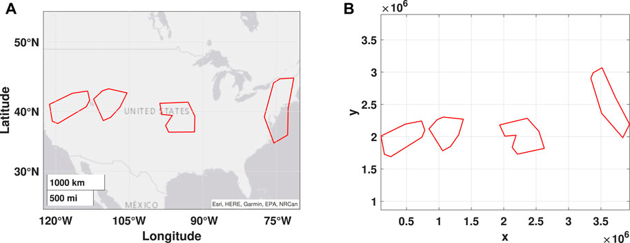
FIGURE 1. Ice hazard data from the aviation weather center taken from 6/23/2022 in (A) latitude/longitude coordinates and (B) Cartesian coordinates.

FIGURE 2

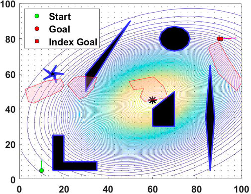
FIGURE 2. A test environment for path planning with dynamic ice obstacles scaled down from Figure 1B.

2.3 Creating training data sets for obstacle dynamics

Starting with the snapshot shown in Figure 1, we emulate obstacle evolution by ascribing simple motions to these shapes. This helps create data sets on which the DMD surrogate models can be trained. It also allows us to evaluate the performance of DMD reduced-order modeling in capturing simple motion types, such as pure translation and changes in size and shape of the obstacle. Figures 3A, 4A, 5A, 6A, 7A, and 8A show different types of training data-sets representing obstacle dynamics of increasing complexity. Figure 3, 4, 5 shows each of the four obstacles decreasing (increasing, mixed rate of change) in size. None of these cases involve translation of the obstacles. Figure 6, 7, 8 shows the obstacles translating as well as decreasing (increasing, mixed rate change) in size. On the right of each of these figures, the performance of the DMD algorithm is shown in capturing these obstacle behaviors. The DMD approach is described in detail in Section 3.2.1. Once the DMD model is trained, it is used to forecast the location and shape of each of the obstacles for future time steps.

FIGURE 3

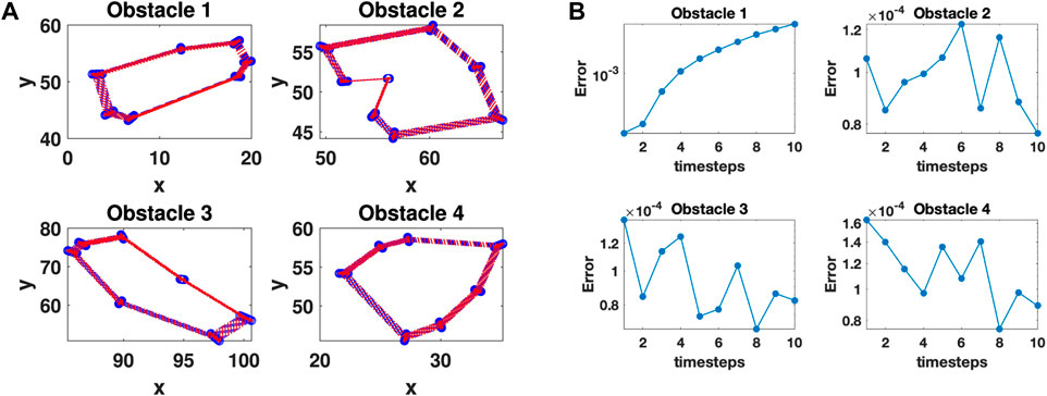
FIGURE 3. (A) Comparative performance of the DMD surrogate modeling for learning shrinking obstacles. Blue depicts ground truth and red depicts DMD output. (B) Validation error characteristics.

FIGURE 4

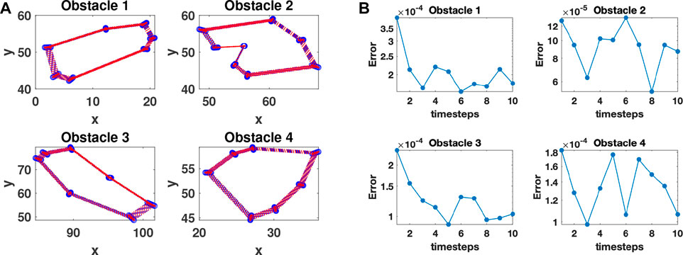
FIGURE 4. (A) Comparative performance of the DMD surrogate modeling for learning expanding obstacles. Blue depicts ground truth and red depicts DMD output. (B) Validation error characteristics.

FIGURE 5

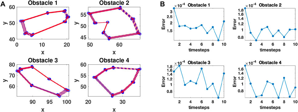
FIGURE 5. (A) Comparative Performance of the DMD Surrogate Modeling for Learning A Mixed Set of Obstacles (Expanding: top right Shrinking: all the rest). Blue Depicts Ground Truth and Red Depicts DMD Output. (B) Validation Error Characteristics.

FIGURE 6

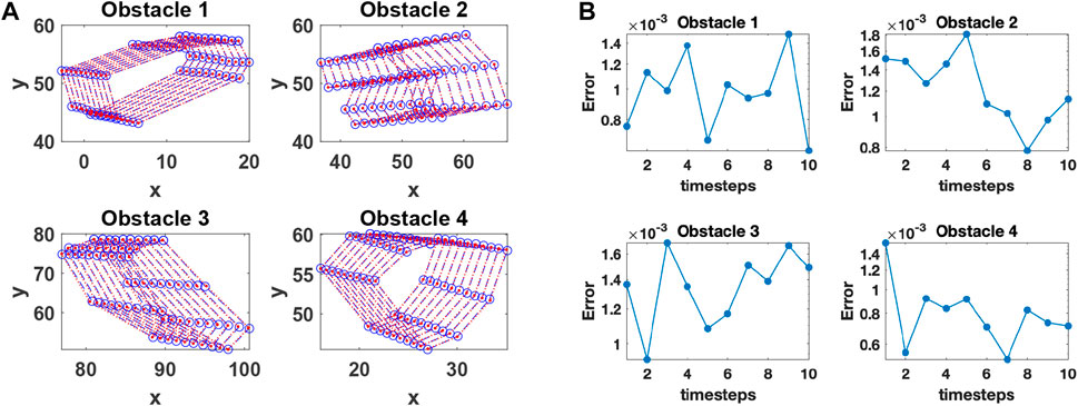
FIGURE 6. (A) Comparative performance of the DMD surrogate modeling for learning obstacles showing pure translation. Blue depicts ground truth and red depicts DMD output. (B) Validation error characteristics.

FIGURE 7

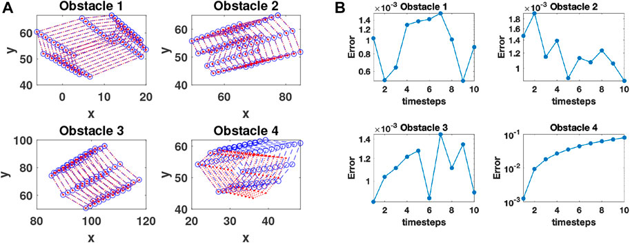
FIGURE 7. (A) Comparative performance of the DMD surrogate modeling for learning obstacles showing translation and expanding size. Blue depicts ground truth and red depicts DMD output. (B) Validation error characteristics.

FIGURE 8

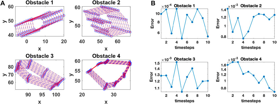
FIGURE 8. (A) Comparative performance of the DMD surrogate modeling for learning obstacles showing translation and mixed changing shape. Blue depicts ground truth and red depicts DMD output. (B) Validation error characteristics.

2.4 Cost and constraint models

The optimal control problem is used to determine the minimum time path to reach the goal when the velocity is held constant. This is shown in Eq. 6 where s is the state vector of the agent shown in Eq. 7.

$J(t,\mathbf{s},u)=\underset{u}{\min }{t}_f(6)$

$\mathbf{s}=(x,y,\psi )(7)$

$\frac{d\mathbf{s}}{dt}=f(x,y,\psi )(8)$

The static obstacles can be modeled as polygons as shown in Eq. 9, where, a_i,j and b_i,j represent the polygon vertices and c_i,j represents the edges of the polygon. The static obstacles are considered to be no-fly-zones that remain constant throughout the search. The dynamic obstacles are no-fly-zones that are changing in each time step as the agent moves towards the goal.

$\underset{j=1}{\overset{M_i}{\bigwedge }}{a}_{i,j}x+b_{i,j}y>c_{i,j}i=1,...,N(9)$

When flying near densely populated environments the noise generated by the vehicle is a factor that must be accounted for. Limiting noise exposure from the aircraft is not a constraint that can be enforced in a point-wise manner as public perception is affected by both noise intensity and duration of disturbance (Administration, 2022). The better way to model noise exposure is with a noise penalty function that is integrated along the vehicle’s flight path. The penalty function has a high value near the population center and lowers as the distance from the population center increases. Placing an upper bound on the accumulation of the noise penalty function over the flight path discourages short flights over the population center with high instantaneous noise, but also penalizes long paths around the population center that generates low noise over long durations. The noise penalty function combined with an upper bound of the accumulated penalty constitutes a path dependant resource constraint which is shown in Eq. 10.

${\int }_0^t{\mathcal{F}}_{\mathcal{L}}(\tau ,\mathbf{s}(\tau ),u(\tau )){\le \mathcal{L}}^{\star }(10)$

The terminal conditions are the initial position and heading of the agent represented by 0, and the final position and heading of the agent represented by t_f. The state boundaries are shown in Eq. 9.

$\text{Terminal\hspace{0.17em}Conditions:\hspace{0.17em}}\{x(0),y(0),\psi (0)\}=\{x_0,y_0,{\psi }_0\}$

$\{x(t_f),y(t_f),\psi (t_f)\}=\{x_f,y_f,{\psi }_f\}(11)$

$\text{State\hspace{0.17em}Bounds:\hspace{0.17em}}{x}_{\mathit{min}}\le x(t)\le x_{\mathit{max}}$

$y_{\mathit{min}}\le y(t)\le y_{\mathit{max}}(12)$

An example of the environment is shown in Figure 2 which shows the terminal conditions labeled as Start and Goal in the graph. The state boundaries for this problem are 0 m for x_min and y_min, and 100 m for the x_max and y_max. The noise penalty function (resource constraint) modeled as a Gaussian distribution is also shown, and the center of the noise penalty function is a black star symbol located at (60, 45). As the agent moves closer to the center of the noise penalty function, the penalty accumulated per action also increases. This is shown by the gradient going from yellow to blue from the center to the edges of the distribution. The mean of the Gaussian distribution is μ_x = 60 and μ_y = 45 which is the center location (60, 45). Other types of contours that could be used are uniform, exponential or from a table (Kim and Hespanha, 2004). Also shown in Figure 2 are the static obstacles, polygons outlined in blue with black fill, and the first step of the dynamic ice obstacles outlined in red with pink fill.

3 Methodology

3.1 Backtracking hybrid A^⋆

Graph search algorithms such as Dijkstra, A^⋆, and Hybrid A^⋆ are popular methods to solve the shortest path problem due to the shorter computation time to reach the goal state. Graph search methods used in motion begin by dividing the environment into cells by grid points or nodes (Fujimura, 1991). Dijkstra is a popular graph search method that was developed in 1959 (Dijkstra, 1959). This method involves creating a grid of the environment with nodes set at equal distance apart from each other. The Dijkstra algorithm is not directed towards the goal and can consequently have lengthy computation time due to this inefficiency. As a result, Dijkstra can be used for an environment for a small amount of nodes (Fujimura, 1991). The A^⋆ algorithm is an evolution of Dijkstra that employs a heuristic function to direct the search towards the goal. In this way, A^⋆ is suitable for a larger environment with more nodes (Fujimura, 1991). The use of the heuristic function increases the efficiency and decreases the nodes that are explored when compared to Dijkstra. A flaw that both of these graph search methods have is that they are constrained to perpendicular turns moving from node to node; this produces paths with sharp angles which cannot be navigated by a vehicle with turn constraints. These turn constraints are due to both the kinematics, the vehicle’s inertia, and the dynamics, or the controls, of the vehicle such as a fixed-wing UAV, cannot navigate. Hybrid A^⋆ is an improvement to the A^⋆ algorithm with the inclusion of the kinematic constraints of the agent with Dubins motion shown in Eq. 2.1 that creates a path that the vehicle can navigate (Richards et al., 2004) (Petereit et al., 2012) (Dolgov et al., 2008). In essence, Hybrid A^⋆ allows for the path to be separated from the grid and produces a path that is smoother and shorter than that of its predecessor A^⋆. Hybrid A^⋆ algorithm though may be unable to find the minimum solution path due to the discretization of the continuous space as well as having to consider different obstacles and constraints (Dolgov et al., 2008)

$\mathcal{D}={\{x_i\}}_{i=1}^{N_x}\otimes {\{y_i\}}_{i=1}^{N_x}\otimes {\{{\psi }_i\}}_{i=1}^{N_x}(13)$

$N_x=|(x_{\mathit{max}}-x_{\mathit{min}})/\delta x|(14)$

$N_y=|(y_{\mathit{max}}-y_{\mathit{min}})/\delta y|(15)$

$N_{\psi }=|({\psi }_{\mathit{max}}-{\psi }_{\mathit{min}})/\delta \psi |(16)$

An auxiliary grid is created $\mathcal{D}$ to keep track of the three-dimensional search space which is the Cartesian coordinates (x, y) and the heading of the agent (ψ). This grid shows the admissible nodes created by the outer product of Eq. 13 where N_x, N_y, and N_ψ are defined as Eq. 14, 15, 16. Due to the manner in which the grid is constructed, the initial position is always located on the grid; this may not be true of the goal position. If the goal position does not land on an auxiliary node from $\mathcal{D}$, it is assigned to the node that it is closest to as the Index Goal which is shown in Figure 2 as the magenta square. The candidate nodes are then coupled with the closest node from the auxiliary grid. Hybrid A^⋆ operates using two sets of nodes; a Frontier (open) set and a visited (closed) set. When a cell is considered “closed”, it is moved to the visited set and is no longer an admissible node for the agent to move to. Therefore, any candidate nodes that end in a closed cell are declared inadmissible. When a cell has been visited by Hybrid A^⋆, all the other potential actions that land in that cell are dismissed. This constrains the explosive growth of the search tree that would occur if the search space was purely continuous. This algorithm only considers all events until the path is found.

Backtracking Hybrid A^⋆ is a recently developed improvement on Hybrid A^⋆ (Ford et al., 2022) to allow for the efficient solution of resource-constrained path planning problems. Backtracking Hybrid A^⋆ operates on the principle that the violation of the loading constraint (Eq. 10) is not the fault of the node in violation, but the fault of the entire path taken to the node. When Backtracking Hybrid A^⋆ encounters a loading constraint violation it backtracks away from the violation. This frees previously explored nodes in the visited set allowing for the re-exploration of a section of the search domain. Because no new child is generated for the node stopped at, the search is forced to take a different path during the re-exploration thus “shedding” some of the load. Repeated invocation of the backtracking procedure during the search allows for rapid load shedding while producing good solutions.

A key aspect of Backtracking Hybrid A^⋆ is how far to backtrack when the loading constraint ${\mathcal{L}}^{\star }$ is violated. This is encapsulated in the backtracking stopping criterion which tells the backtracking procedure to halt its backward March. Stopping criteria are heuristic in nature and often attempt to use information from the loading function as well as the graph structure. The stopping criterion used in this work is called load rate stopping which seeks to maximize the sensitivity of rate of load accumulation with respect to the heading rate along the search path. This can be stated as follows:

$s^{*}={\max }_{\tau ϵ(0,t)}\frac{{\partial \mathcal{F}}_{\mathcal{L}}(\tau ,\mathbf{s}(\tau ),u(\tau ))}{\partial \dot{\psi }}(17)$

where s∗ is the pose along the path to the invalid node where the change in load accumulation with respect to heading rate is maximized. This can be applied to Hybrid A^⋆ by taking the rate of load accumulation to be the load accumulated on edge leading to a given node, and varying the turning rate as the choice between three motion primitives. This means that re-exploration initiates where there the potential for changing the total load incurred by the search is maximised.

3.2 Dynamic mode decomposition

Dynamic Mode Decomposition (DMD) is a data-driven approach to discover system models, based on the theory of Koopman operators. Its primary advantage is that it casts the unknown system as a linear model in a transformed space of observables, thereby facilitating downstream analysis and increasing the possibility of achieving performance guarantees. Koopman operator theory was first introduced in the 1930s and has since gained popularity over the past two decades (Koopman, 1931; Koopman and Neumann, 1932). The renewed interest in this theory was primarily driven by recent advances in numerical methods through Koopman analysis, one such method is Dynamic Mode Decomposition (DMD) (Rowley et al., 2009; Schmid, 2010). DMD has been designed to effectively capture the low-order dynamics of a complex system and perform future predictions. It does so by superimposing the empirically computed DMD modes and corresponding DMD frequencies of the underlying system. Generally, the number of modes required to describe the system is significantly smaller than the dimension of the actual data set. Apart from the benefit of reduced computational effort, one primary advantage of DMD is its “equation free” nature. As a result, one does not need to know the complicated underlying physics and can model the system purely from data.

3.2.1 The DMD algorithm

In our work, we have used the exact DMD algorithm developed by Tu and collaborators (Tu et al., 2013; Kutz et al., 2016). DMD requires a pair of snapshot matrices in order to generate a linear model approximating the desired dynamical system. We sample the state x at different time instants (snapshots) and stack them to form snapshot matrices X and X′, where X′ is just one snapshot ahead of the original snapshot matrix X.

$\begin{array}{ll}\hfill X& =\left[\begin{array}{ccccc}\hfill x(t_0)\hfill & \hfill x(t_1)\hfill & \hfill x(t_2)\hfill & \hfill ...\hfill & \hfill x(t_{m-1})\hfill \end{array}\right]\hfill \\ \hfill X^{\prime }& =\left[\begin{array}{ccccc}\hfill x(t_1)\hfill & \hfill x(t_2)\hfill & \hfill x(t_3)\hfill & \hfill ...\hfill & \hfill x(t_m)\hfill \end{array}\right]\hfill \end{array}(18)$

In Eq. 18 t_k+1 = t_k + Δt, where k = 0, 1, …, m and Δt is the time step between two consecutive snapshots. Without loss of generality, we can assume that the snapshots start from t = 0, i.e. t₀ = 0. Under the assumption of uniform sampling, t_m = mΔt. The DMD algorithm seeks the best fit linear operator A in least-square sense that relates the two snapshot matrices such that

$\begin{array}{ll}\hfill X^{\prime }& \approx AX,\hfill \end{array}(19)$

and attempts to extract the eigenvalues and eigenvectors of A in an efficient manner. The A matrix resembles the finite-dimensional discrete-time Koopman operator where we choose our state variables as the observables, i.e., g(x) = x, where g is the observable or measurement function. Our objective is to find the eigenvalues and eigenvectors of A and use them to model the time evolution of our state variables. It is not necessary that we use the entire data set to build the snapshot matrices; DMD allows us to sample the original data set in a flexible manner, for example in a randomized approach to select a suitable sampling region (Erichson et al., 2019). In the current problem, the snapshot matrices are created by stacking the Cartesian coordinates of the polygonal shapes representing the ice hazards over the training time horizon. The DMD algorithm itself can be broken down into five steps.

• Step 1: Singular value decomposition (SVD) of snapshot matrix X,

$\begin{array}{ll}\hfill X& =U\mathrm{\Sigma }{V}^T\approx U_r{\mathrm{\Sigma }}_r{V}_r^T,\hfill \end{array}(20)$

where U contains the left singular vectors, Σ is a diagonal matrix of singular values arranged in a hierarchical manner and V contains the right singular vectors. In practice, it is sufficient to compute the reduced SVD, where only first few (r) columns and rows of respectively U and V are retained with first r singular values of Σ. The SVD energy thresholding algorithm is used to determine r and then truncate our U, Σ and V matrices accordingly (Kutz, 2013).

• Step 2: A is obtained by

$\begin{array}{ll}\hfill A& =X^{\prime }{X}^{†}=X^{\prime }{V}_r{\mathrm{\Sigma }}_r^{-1}{U}_r^T\hfill \end{array}(21)$

A is then projected onto a lower dimensional space using a similarity transformation,

$\begin{array}{ll}\hfill A_r& =U_r^{T}A{U}_r=U_r^T{X}^{\prime }{V}_r{\mathrm{\Sigma }}_r^{-1}.\hfill \end{array}(22)$

An important observation here is that the eigenvalues of A are adequately approximated by the eigenvalues of A_r.

• Step 3: The spectral decomposition of A_r is computed,

$\begin{array}{ll}\hfill A_{r}W& =W\mathrm{\Lambda }\hfill \end{array}(23)$

W is the matrix of eigenvectors of A_r and Λ is the diagonal matrix containing its eigenvalues.

• Step 4: The DMD modes are given by the columns of Φ,

$\begin{array}{ll}\hfill \mathrm{\Phi }& =X^{\prime }{V}_r{\mathrm{\Sigma }}_r^{-1}W\hfill \end{array}(24)$

These DMD modes approximate the eigenvectors of the high dimensional matrix A (Tu et al., 2013; Kutz et al., 2016).

• Step 5: Finally, the DMD predicted state $\widehat{x}(t)$ at any time t is given by

$\begin{array}{ll}\hfill \widehat{x}(t)& =\mathrm{\Phi }\exp (\mathrm{\Omega }t)b\hfill \end{array}(25)$

where b = Φ^†x₀, and x₀ = x (t₀).

     x₀ is the first column of X and, Ω is the vector of DMD frequencies (ω) which are obtained from DMD eigenvalues using the relation $\omega =\frac{\ln \mid \lambda \mid }{\mathrm{\Delta }t}$, with λ being the diagonal elements of Λ.

The DMD algorithm was incorporated into the Hybrid A^⋆ with backtracking path planner as a way to predict the time evolution of the dynamics of the ice obstacles. DMD will predict the motion past the original ten time steps from the Aviation Weather Service (AWS) data. For this particular data set, DMD continued to predict the motion of the obstacles for a total of 100 time steps forward in time. The snapshot matrices are created by using vertex location of the obstacles at each time step. The first ten time steps are modeled to recreate how the ice phenomena would change based on initial conditions from AWS, this is a limitation as we apply a data driven technique on simulated data rather than the actual data itself. Techniques to overcome this limitation will be addressed in future work. Since AWS data is continuously updated, an online DMD method can also be applied to check the DMD’s applicability in real-time Zhang et al. (2019); Nayak et al. (2021a) for the time-varying AWS data.

4 Results

This section presents path-planning results with static and dynamic obstacles and a resource constraint. All computations are performed on an AMD Ryzen 9 5900HX CPU with Radeon Graphics at 3.30 GHz and 16.0 GB RAM on a Microsoft Windows system using MATLAB® version R2022a. The map is bound by the 0–100 m in the x and y direction. The initial pose O = (10, 5, 90°) is shown as the green dot, and the final pose G = (90, 80, 0°) is shown as the red dot for the cases. The agent has a turn radius of 8 m and a velocity of 3 m/s. The $\mathcal{D}$ auxiliary grid was created using the agent’s constraints as shown by δx = δy = 3 m and δψ = 0.375rad. All cases contain six static obstacles outlined in blue and filled in with black. There is one Gaussian distribution acting as the noise level constraint that the agent must be able to satisfy. The magenta square is the closed node of grid $\mathcal{D}$ closest to the goal.

AWS ice hazard data from 23 June 2022 was used in this paper (red outlined with pink fill) as the starting location and shape of the dynamic obstacles. Various cases of obstacle dynamics were considered. These are labeled in Tables 1, 2 under the column “Motion Type” column. The first letter is either “D”, for decreasing, “I”, for increasing, and “B” for both increasing and decreasing obstacles (mixed obstacle type). “NT” stands for no translation motion, and “T” stands for translation motion. The evolution of the dynamic ice obstacles is shown by gray outlines. The results of DMD reduced order modeling of these obstacles’ dynamics are shown in Figures 3–8. The left plots on Figures 3–8 illustrate the first ten time steps of the ground truth obstacle dynamics (shown in blue) and their DMD reconstruction (shown in dotted red). The right plots show the DMD mean relative two norm error of the approximation to training data for each obstacle. The DMD approach is able to recreate the ground truth with a high degree of accuracy. The total time taken to learn the surrogate dynamics for all six cases is on the order of 1 min. As a benchmark, the same cases were run on the Hybrid A^⋆ without backtracking. The algorithm was unable to find the path for all six cases. The time it took for the algorithm to end is recorded in Table 1, in the range of 10–15 s.Results of six separate cases are shown in Table 2. These are described individually below.

• Case 1. This is a “DNT” scenario, shown in Figure 9. In other words, the dynamic obstacles are all decreasing in size and not translating. The $\mathcal{BH}{A}^{*}$ algorithm is able to reach its goal pose in 5.31 s (compute time), returning a path length of 143.99 units. During the graph search process, the resource constraint is violated on numerous occasions, triggering the backtracking routine. There were a total of 339 instances of backtracking performed in this search. Note that this case is “easy” in the sense that all obstacles decrease in size over time, clearing up more flight space as time passes.

• Case 2. This is a “INT” scenario in which the obstacles all expand so rapidly that they overlap beyond a certain point before the agent can pass through in between them (see snapshot 33 of 50 in Figure 10). The agent is unable to pass between the two obstacles in the middle because of the resource constraint. Eventually, the obstacle on the right nearly engulfs the goal location such that it is not possible to achieve the desired pose of 0 deg heading. In this case involving aggressively expanding dynamic obstacles, no solution exists.

• Case 3. This represents a “BNT” scenario with a mixture of expanding and shrinking obstacles, none translating (see Figure 11). The goal is reached with a path length, compute time and backtracking characteristics that are comparable to Case 1 (see Table 2). This is because the “active” obstacles (the two on the left) behave in the same way as Case 1.

• Cases 4–6. All of these scenarios include translational motion of the obstacles. Figure 12 considers shrinking obstacles (scenario “DT”), Figure 13 considers growing obstacles; Figure 14 considers a mixed collection of obstacles in addition to translation. All cases are able to reach the goal with characteristics as shown in Table 2.

It is not surprising that the scenarios involving obstacles of growing size require the backtracking procedure to be activated most frequently (702 backtracking instances required for “INT”, without success, of course). The optimization routine tries its best to find a keyhole trajectory between the two obstacles in the middle of the domain as the other options are closed out due to overlapping obstacles. However, the open region between the two obstacles in the middle is also a region of heavy loading, causing multiple failed attempts at backtracking. The most benign case for backtracking is “DT” as the obstacles decrease in size and generally tend to steer clear of the UAV’s path. Finally, note that the compute time for all scenarios that admit a valid solution is relatively small. Numbers shown in this Table do not include the time taken to learn the DMD reduced order models of the obstacles (adds a few additional seconds, less than 10 s per case). Recall that resource constrained path planning is NP hard and while the optimal solution can be found using mixed integer linear programming (MILP), the computational load is prohibitive. Alternatively, the Lagrange Relaxation approach Ahujia et al. (1993); Bertsekas (1999) can be employed to transform the problem into a dual problem that leads to a relaxation of the constraint coupling. It uses Dijkstra’s algorithm in an iterative manner by modifying the edge weights until the constraint is met. While the LARAC approach improves upon the MILP formulation, it still requires two orders of magnitude greater compute time that the proposed backtracking method. Graph search without backtracking (e.g., traditional hybrid A∗) is either severely suboptimal or simply infeasible because of the naive manner in which it classifies nodes as inadmissible.

TABLE 1

TABLE 1. Hybrid A^⋆ results with ice dynamic obstacles.

TABLE 2

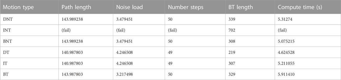
TABLE 2. Backtracking hybrid A^⋆ results with ice dynamic obstacles.

FIGURE 9

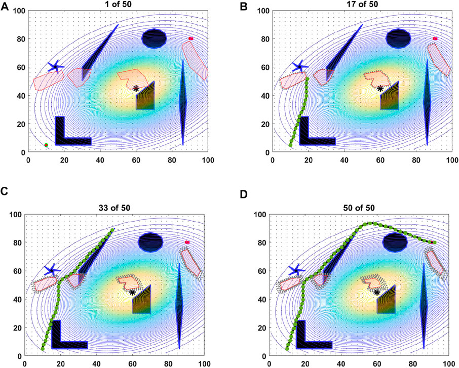
FIGURE 9. Four snapshots (A-D) of the path-planning process for the case with shrinking obstacles and no translational motion.

FIGURE 10

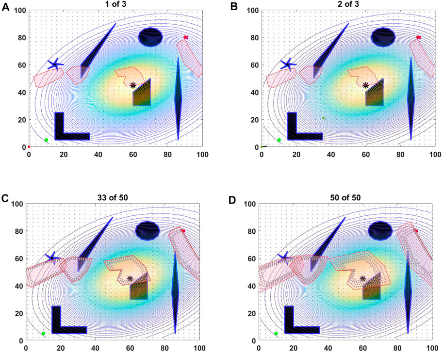
FIGURE 10. Four snapshots (A-D) of the path-planning process for the case with expanding obstacles and no translational motion. Note that no solution is found as obstacles overlap (C, D) and the resource constraint dominates open gaps.

FIGURE 11

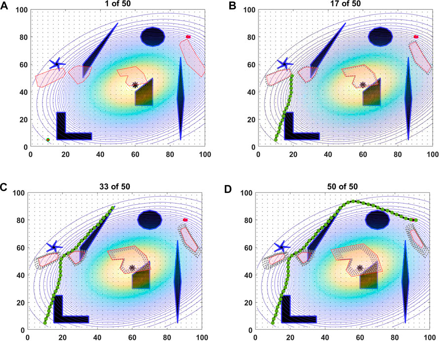
FIGURE 11. Four snapshots (A-D) of the path-planning process for the case with expanding and shrinking obstacles and no translational motion.

FIGURE 12

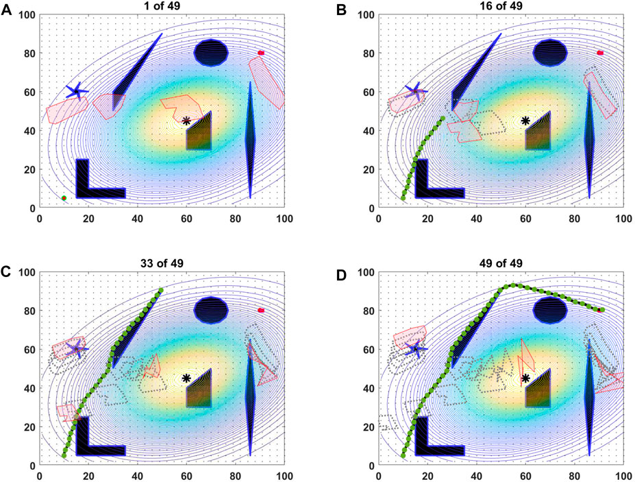
FIGURE 12. Four snapshots (A-D) of the path-planning process for the case with shrinking obstacles and translational motion. This is the most benign planning scenario.

FIGURE 13

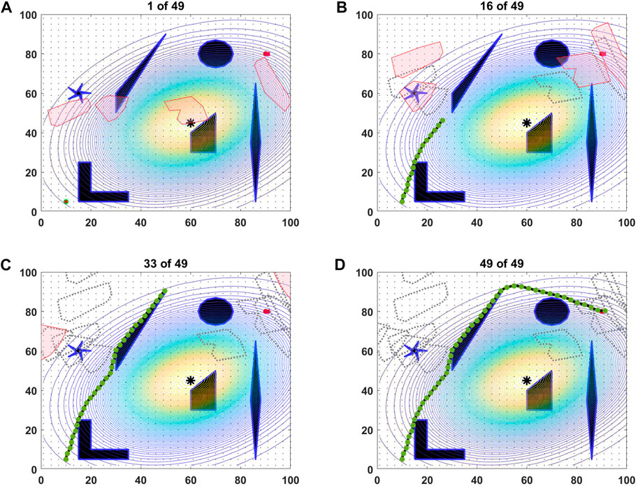
FIGURE 13. Four snapshots (A-D) of the path-planning process for the case with expanding obstacles and translational motion.

FIGURE 14

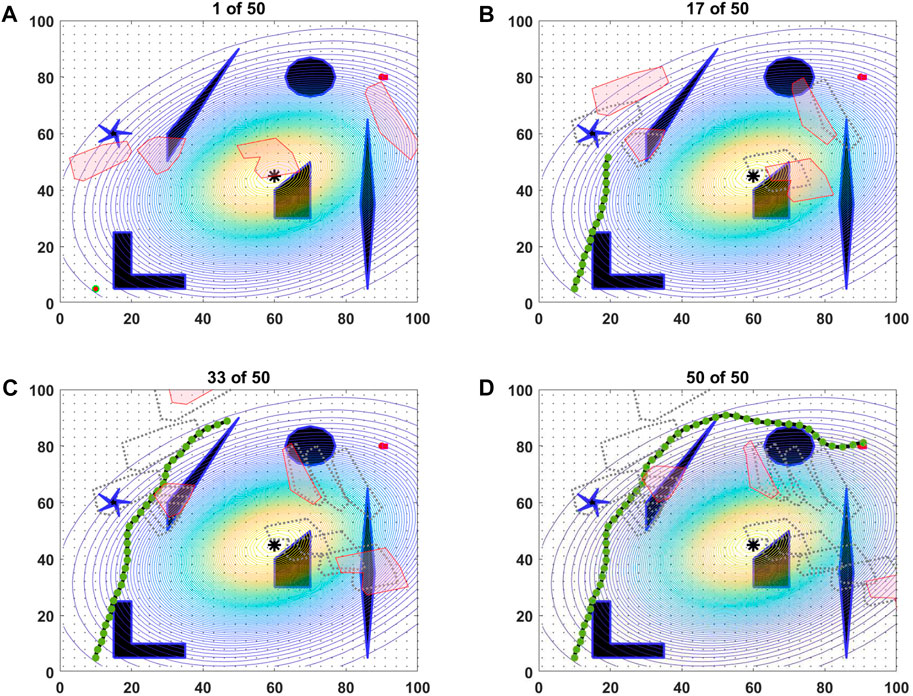
FIGURE 14. Snapshots of the Path-Planning Process for the Case with Shrinking and Expanding Obstacles as well as Having Translational Motion. (A) DNT, (B) DT, (C) INT, (D) IT, (E) BNT. (F) BT.

The load accumulated by the noise constraint is shown for the six cases in Table 2 under the “Noise Load” column. For each case that reached the goal, the load was below the maximum constraint of 6. The backtracked paths for each of the six cases are shown on the plots of Figure 15. The green line is the path that the agent took from the start to the goal node, while the blue and orange lines are the backtracked paths that the agent did not take. The blue and orange paths are to better visual the backtracked paths, to differentiate the different backtracked paths. The blue lines show the full backtracked path, while the orange is showing where the backtrack path begins. While the dynamic obstacles moved in different directions and grew or shrank in each case, the path planner found similar paths with loading of the noise constraint and the path length to be in the same magnitude. The time is for each case is 4–6 s.

FIGURE 15

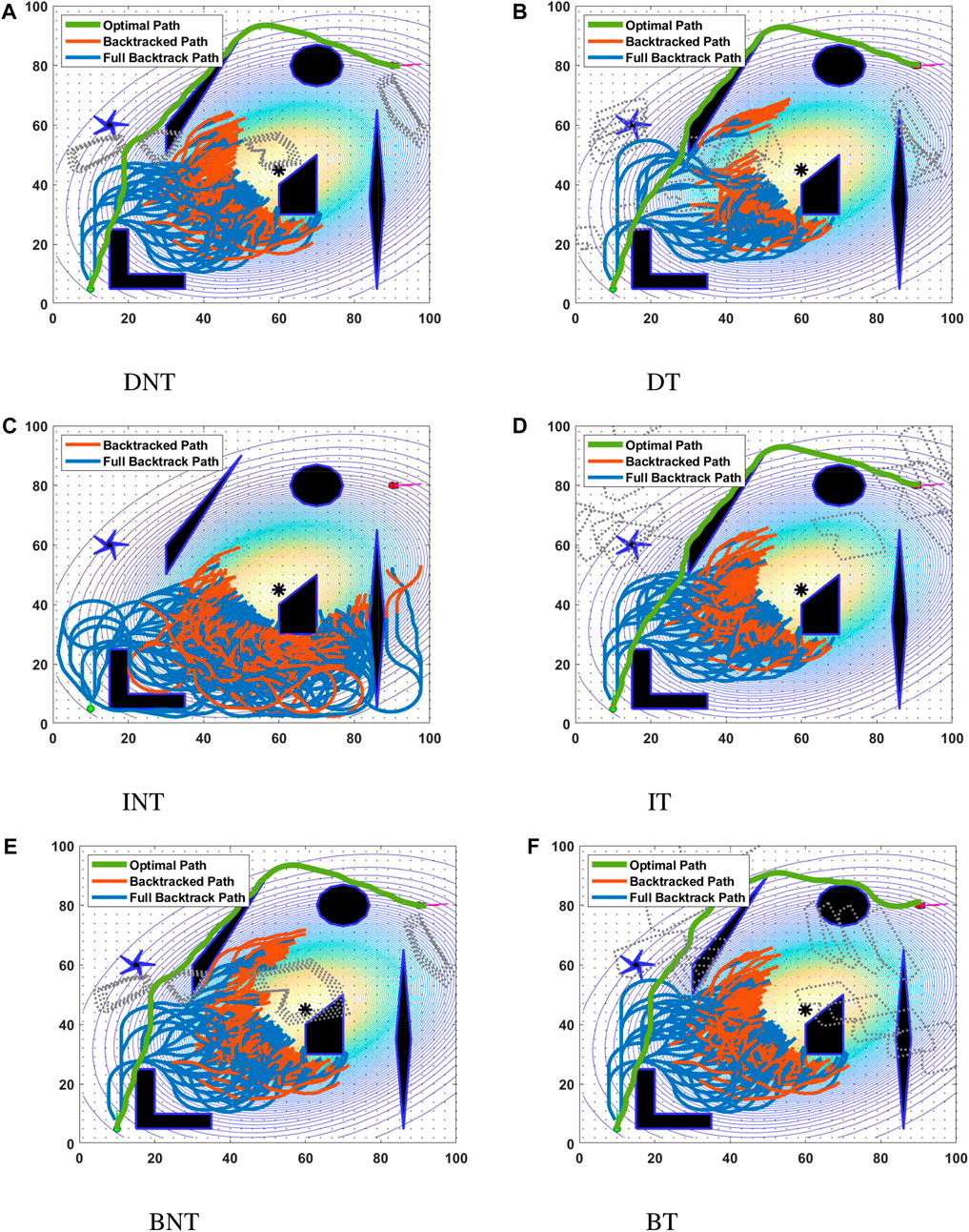
FIGURE 15. Illustration of backtracking performed in all six path-planning scenarios: (A) DNT, (B) DT, (C) INT, (D) IT, (E) BNT, and (F) BT. The orange paths indicate the point during the backtracking process that the stopping criterion was met.

As a final note, we point out that it is very easy to construct scenarios in which $\mathcal{BH}{A}^{*}$ will fail to generate a solution, e.g., an obstacle that expands rapidly to fill up most of the solution space. In cases like these, the presented approach as no mechanism to “pick-up” the search from a previously concluded search that ended in premature failure. We remind the reader that in this work, each instance of path-planning is considered as a stand-alone problem and there is no provision for re-planning. In its current state, the presented work is purely academic. An elaborate testing plan (both in simulation environments and actual flight tests) is needed to achieve the verification and validation of the proposed methodology. Results in this section demonstrate scalability of the presented approach. It is flight readiness will only be ascertained through rigorous testing in hardware.

5 Conclusion

This paper considers path planning with resource constraints and dynamic obstacles for a Dubins agent. Path planning with dynamic obstacles and resource constraints creates a more realistic model of what an agent will encounter during its missions. A DMD reduced-order modeling approach is developed to learn obstacle dynamics for a range of translational and shape deformation motions. The forecast location and shape of dynamic obstacles is provided to a backtracking hybrid A∗ search for determination of the shortest path to the agent’s goal pose. The backtracking hybrid-A∗ algorithm is able to handle path-dependent resource constraints by receding the graph search when the resource constraint is violated. This allows load-shedding, leading to rapid discovery of keyholes around regions of high path loading.

While this study used initial ice data from the Aviation Weather Service (AWS), there is room for additional research in applying DMD recursively to AWS to better capture obstacle dynamics. The overall compute time of the proposed methodology is low compared to existing techniques for resource-constrained problems.

Future work includes further improvement in the efficiency of the algorithm in a 2D environment and integration of dynamic obstacles in a 3D environment. This entails improving the backtracking stopping criterion, and integration of the backtracking approach with other optimal path-planning techniques. Other areas of improvement include adding a re-planning module that can leverage results from previous cycles of planning. Of course, there is also the problem of flight integration and eventual certification of the presented path-planning approach through rigorous verification and validation techniques.

Data availability statement

The raw data supporting the conclusion of this article will be made available by the authors, without undue reservation.

Author contributions

AC: Coding DMD reduced order modeling, acquiring data from Aviation Weather Service, integrating all code and generating results, writing paper. BF: Developing and coding the backtracking hybrid A∗. IN: Support for DMD and writing Section 3.2. SN: Development support for DMD and writing Section 3.2. MK: Coordinating all research, acquiring funding for work, writing and revising the manuscript.

Funding

The authors acknowledge support from the National Science Foundation award number 2132798 under the NRI 3.0: Innovations in Integration of Robotics Program.

Conflict of interest

The authors declare that the research was conducted in the absence of any commercial or financial relationships that could be construed as a potential conflict of interest.

Publisher’s note

All claims expressed in this article are solely those of the authors and do not necessarily represent those of their affiliated organizations, or those of the publisher, the editors and the reviewers. Any product that may be evaluated in this article, or claim that may be made by its manufacturer, is not guaranteed or endorsed by the publisher.

References

Administration, F. A. (2022). Faa history of noise. (Last accessed June 18, 2022).

Google Scholar

Administration, F. A. (2010). Federal aviation administration advisory circular, ac 00-45g, change 1. (Last accessed Apr 7, 2022).

Google Scholar

Administration, F. A. (2020). How to properly use an icing forecast - aviation weather. (Last accessed Apr 7, 2022).

Google Scholar

Ahujia, R., Magnanti, T. L., and Orlin, J. B. (1993). Network flows: Theory, algorithms and applications. New Jersey: Rentice-Hall.

Google Scholar

Banzhaf, H., Berinpanathan, N., Nienhüser, D., and Marius Zöllner, J. (2018). “From g2 to g3 continuity: Continuous curvature rate steering functions for sampling-based nonholonomic motion planning,” in In 2018 IEEE intelligent vehicles symposium, 326–333. doi:10.1109/IVS.2018.8500653

CrossRef Full Text | Google Scholar

Bertsekas, D. P. (1999). Nonlinear programming.

Google Scholar

Botros, A., and Smith, S. L. (2022). Tunable trajectory planner using g3 curves. IEEE Trans. Intelligent Veh. 1, 273–285. doi:10.1109/TIV.2022.3141881,

CrossRef Full Text | Google Scholar

Broatch, A., García-Tíscar, J., Roig, F., and Sharma, S. (2019). Dynamic mode decomposition of the acoustic field in radial compressors. Aerosp. Sci. Technol. 90, 388–400. doi:10.1016/j.ast.2019.05.015

CrossRef Full Text | Google Scholar

Darbari, V., Gupta, S., and Verma, O. P. (2017). “Dynamic motion planning for aerial surveillance on a fixed-wing uav,” in 2017 international conference on unmanned aircraft systems (ICUAS), 488–497. doi:10.1109/ICUAS.2017.7991463

CrossRef Full Text | Google Scholar

Dijkstra, E. W. (1959). A note on two problems in connexion with graphs. Numer. Math. 1, 269–271. doi:10.1007/bf01386390

CrossRef Full Text | Google Scholar

Dolgov, D. A., Thrun, S., Montemerlo, M., and Diebel, J. (2008). Practical search techniques in path planning for autonomous driving.

Google Scholar

Dubins, L. E. (1957). On curves of minimal length with a constraint on average curvature, and with prescribed initial and terminal positions and tangents. Am. J. Math. 79, 497. doi:10.2307/2372560

CrossRef Full Text | Google Scholar

Erichson, N. B., Mathelin, L., Kutz, J. N., and Brunton, S. L. (2019). Randomized dynamic mode decomposition. SIAM J. Appl. Dyn. Syst. 18, 1867–1891. doi:10.1137/18m1215013

CrossRef Full Text | Google Scholar

Ford, B., Aggarwal, R., Kumar, M., Manyam, S. G., Casbeer, D., and Grymin, D. (2022). “Backtracking hybrid Α* for resource constrained path planning,” in AIAA SCITECH 2022 forum, 1–19. doi:10.2514/6.2022-1592

CrossRef Full Text | Google Scholar

Fujimura, K. (1991). Motion planning in dynamic environments. Springer-Verlag.

Google Scholar

Han, Y., and Tan, L. (2020). Dynamic mode decomposition and reconstruction of tip leakage vortex in a mixed flow pump as turbine at pump mode. Renew. Energy 155, 725–734. doi:10.1016/j.renene.2020.03.142

CrossRef Full Text | Google Scholar

Kabamba, P. T., Meerkov, S. M., and Zeitz, F. H. (2006). Optimal path planning for unmanned combat aerial vehicles to defeat radar tracking. J. Guid. Control, Dyn. 29, 279–288. doi:10.2514/1.14303

CrossRef Full Text | Google Scholar

Kim, J., and Hespanha, J. (2004). “Discrete approximations to continuous shortest-path: Application to minimum-risk path planning for groups of uavs,” in 42nd IEEE conference on decision and control, 2, 1734–1740. doi:10.1109/CDC.2003.1272863

CrossRef Full Text | Google Scholar

Koopman, B., and Neumann, J. v. (1932). Dynamical systems of continuous spectra. Proc. Natl. Acad. Sci. U. S. A. 18, 255–263. doi:10.1073/pnas.18.3.255

PubMed Abstract | CrossRef Full Text | Google Scholar

Koopman, B. O. (1931). Hamiltonian systems and transformation in hilbert space. Proc. Natl. Acad. Sci. U. S. A. 17, 315–318. doi:10.1073/pnas.17.5.315

PubMed Abstract | CrossRef Full Text | Google Scholar

Kutz, J. N., Brunton, S. L., Brunton, B. W., and Proctor, J. L. (2016). Dynamic mode decomposition: Data-driven modeling of complex systems (SIAM).

Google Scholar

Kutz, J. N. (2013). Data-driven modeling & scientific computation: Methods for complex systems & big data. Oxford University Press.

Google Scholar

LaValle, S. M. (2006). Planning algorithms. Cambridge: Cambridge University Press. doi:10.1017/CBO97805115468

CrossRef Full Text | Google Scholar

Manyam, S., Rathinam, S., Casbeer, D., and Garcia, E. (2017). Tightly bounding the shortest dubins paths through a sequence of points. J. Intell. Robot. Syst. 495, 495–511. doi:10.1007/s10846-016-0459-4

CrossRef Full Text | Google Scholar

Nayak, I., Kumar, M., and Teixeira, F. (2021a). “Detecting equilibrium state of dynamical systems using sliding-window reduced-order dynamic mode decomposition,” in AIAA scitech 2021 forum, 1858.

CrossRef Full Text | Google Scholar

Nayak, I., Kumar, M., and Teixeira, F. L. (2021b). Detection and prediction of equilibrium states in kinetic plasma simulations via mode tracking using reduced-order dynamic mode decomposition. J. Comput. Phys. 447, 110671. doi:10.1016/j.jcp.2021.110671

CrossRef Full Text | Google Scholar

Nayak, I., and Teixeira, F. L. (2022). “Data-driven modeling of high-q cavity fields using dynamic mode decomposition,” in 2022 IEEE international symposium on antennas and propagation and USNC-ursi radio science meeting (Denver, CO: AP-S/URSI), 10-15 July, 2022, 1118–1119. doi:10.1109/AP-S/USNC-URSI47032.2022.9886176

CrossRef Full Text | Google Scholar

Oliveira, R., Lima, P., Cirillo, M., Mårtensson, J., and Wahlberg, B. (2018). “Trajectory generation using sharpness continuous dubins-like paths with applications in control of heavy duty vehicles,” in 2018 European control conference (ECC), 1–17. doi:10.23919/ECC.2018.8550279

CrossRef Full Text | Google Scholar

Petereit, J., Emter, T., Frey, C. W., Kopfstedt, T., and Beutel, A. (2012). “Application of hybrid a* to an autonomous mobile robot for path planning in unstructured outdoor environments,” in ROBOTIK 2012; 7th German conference on Robotics, 1–6.

Google Scholar

Phillips, M., and Likhachev, M. (2011). “Sipp: Safe interval path planning for dynamic environments,” in Icra, 5628–5635.

CrossRef Full Text | Google Scholar

Reeds, J. A., and Shepp, L. A. (1990). Optimal paths for a car that goes both forwards and backwards. Pac. J. Math. 145, 367–393. doi:10.2140/pjm.1990.145.367

CrossRef Full Text | Google Scholar

Richards, N., Sharma, M., and Ward, D. (2004). “A hybrid a*/automaton approach to on-line path planning with obstacle avoidance,” in AIAA 1st intelligent systems technical conference, 1–17. doi:10.2514/6.2004-6229

CrossRef Full Text | Google Scholar

Rowley, C. W., Mezić, I., Bagheri, S., Schlatter, P., and Henningson, D. S. (2009). Spectral analysis of nonlinear flows. J. Fluid Mech. 641, 115–127. doi:10.1017/S0022112009992059

CrossRef Full Text | Google Scholar

Schmid, P. J. (2010). Dynamic mode decomposition of numerical and experimental data. J. fluid Mech. 656, 5–28. doi:10.1017/s0022112010001217

CrossRef Full Text | Google Scholar

Schmid, P. J., Li, L., Juniper, M., and Pust, O. (2011). Applications of the dynamic mode decomposition. Theor. Comput. Fluid Dyn. 25, 249–259. doi:10.1007/s00162-010-0203-9

CrossRef Full Text | Google Scholar

Shkel, A. M., and Lumelsky, V. (2001). Classification of the dubins set. Robotics Aut. Syst. 34, 179–202. doi:10.1016/S0921-8890(00)00127-5

CrossRef Full Text | Google Scholar

Thomas, B. W., Calogiuri, T., and Hewitt, M. (2019). An exact bidirectional a^⋆ approach for solving resource-constrained shortest path problems. Networks 73, 187–205. doi:10.1002/net.21856

CrossRef Full Text | Google Scholar

Tu, J. H., Rowley, C. W., Luchtenburg, D. M., Brunton, S. L., and Kutz, J. N. (2013). On dynamic mode decomposition: Theory and applications. arXiv preprint arXiv:1312.0041.

Google Scholar

Zabarankin, M., Uryasev, S., and Murphey, R. (2006). Aircraft routing under the risk of detection. Nav. Res. Logist. (NRL) 53, 728–747. doi:10.1002/nav.20165

CrossRef Full Text | Google Scholar

Zhang, H., Rowley, C. W., Deem, E. A., and Cattafesta, L. N. (2019). Online dynamic mode decomposition for time-varying systems. SIAM J. Appl. Dyn. Syst. 18, 1586–1609. doi:10.1137/18m1192329

CrossRef Full Text | Google Scholar