
94% of researchers rate our articles as excellent or good
Learn more about the work of our research integrity team to safeguard the quality of each article we publish.
Find out more
REVIEW article
Front. Astron. Space Sci. , 11 July 2023
Sec. Stellar and Solar Physics
Volume 10 - 2023 | https://doi.org/10.3389/fspas.2023.1159166
This article is part of the Research Topic Reviews in Astronomy and Space Sciences View all 27 articles
 Ming Xiong1,2,3*
 Xueshang Feng1,3
 Bo Li4
 Jiansen He5
 Wei Wang1
 Yanchen Gao1,2
 Man Zhang1
 Liping Yang1
 Zhenghua Huang4
 Jun Cheng1Cang Su1
 Yihua Yan1,2Kairan Ying6*
Interplanetary scintillation (IPS) refers to random fluctuations in radio intensity of distant small-diameter celestial object, over time periods of the order of 1 s. The scattering and scintillation of emergent radio waves are ascribed to turbulent density irregularities transported by the ubiquitous solar wind streams. The spatial correlation length of density irregularities and the Fresnel radius of radio diffraction are two key parameters in determining the scintillation pattern. Such a scintillation pattern can be measured and correlated between multi-station radio telescopes on the Earth. Using the “phase-changing screen” scenario based on the Born approximation, the bulk-flow speed and turbulent spectrum of the solar wind streams can be extracted from the single-station power spectra fitting and the multi-station cross-correlation analysis. Moreover, a numerical computer-assisted tomography (CAT) model, iteratively fit to a large number of IPS measurements over one Carrington rotation, can be used to reconstruct the global velocity and density structures in the inner heliosphere for the purpose of space weather modelling and prediction. In this review, we interpret the underlying physics governing the IPS phenomenon caused by the solar wind turbulence, describe the power spectrum and cross correlation of IPS signals, highlight the space weather application of IPS-CAT models, and emphasize the significant benefits from international cooperation within the Worldwide IPS Stations (WIPSS) network.
The solar wind escapes from the Sun, travels at a supersonic and super-Alfvénic speed, permeates interplanetary space, and ultimately fills the whole heliosphere. The ion species of the solar wind plasma include protons, alpha particles, and minor heavy ions. The solar wind was intuitively conceived as a result of hot coronal expansion. The Alfvén surface is the locus where the radial motion of the accelerating solar wind passes the radial Alfvén speed. The sub-Alfvénic solar wind in the inner heliosphere was firstly measured by Parker Solar Probe (PSP) during its 8th and 9th solar encounters, at a distance of ≈ 16 solar radii (R⊙) from the Sun. The first in situ detections enabled by PSP reveal the distinct nature of turbulence, anisotropy, intermittency, and directional switchback properties of these sub-Alfvénic winds (Kasper et al., 2019). According to PSP observation during encounter 8, the magnetic field and flow velocity vectors were highly aligned in the sub-Alfvénic solar wind (Zank et al., 2022). The solar wind in the heliosphere was locally sampled by Ulysses along its out-of-ecliptic orbit. According to the Ulysses’ fast-latitudinal scan between ± 80°, the distribution of the solar wind within the heliosphere is clearly bimodal, with differing compositions, temperatures, temperature anisotropies, speeds, small scale fluctuations (McComas et al., 2002). At solar maxima, this bimodal configuration gives way to a more complex mixture of slow and fast streams at all heliospheric latitudes, depending on the distribution of open and closed magnetic regions and the highly tilted magnetic polarity inversion line. The background solar wind flow is frequently disturbed by coronal mass ejections (CMEs), large-scale expulsions of plasma and magnetic field from the solar atmosphere. CMEs cause phenomena on the Earth such as geomagnetic storms and solar energetic particles that can result in major space weather effects (Forbes et al., 2006). As CMEs are the main driver of interplanetary and geomagnetic disturbances, interplanetary space can be considered as a transmission channel of hazardous space weather effects connecting the Sun and the Earth. The space weather chain between the CME initiation at the Sun and its ensuing disturbance at 1 AU can be quantitatively studied via global three-dimensional (3D) magnetohydrodynamic (MHD) simulations of the heliosphere such as Space Weather Modeling Framework (SWMF) (Tóth et al., 2005), Conservation Element and Solution Element (CESE)-MHD model (Feng et al., 2010; Feng, 2020), CORona-HELiosphere (CORHEL) (Riley et al., 2012), and EUropean Heliospheric FORecasting Information Asset (EUHFORIA) (Pomoell and Poedts, 2018), ENLIL-Cone model (Odstrcil et al., 2004), Multi-Scale FLUid-Kinetic Simulation Suite (MS-FLUKSS) flux-rope model (Singh et al., 2019), Grid Agnostic MHD for Extended Research Applications (GAMERA) (Merkin et al., 2016). Presently, and in the foreseeable future, numerical models based on the 3D MHD equations are the only self-consistent mathematical descriptions that can span the enormous distances associated with large-scale space weather phenomena (De Zeeuw et al., 2000).
The currently observable signatures of interplanetary solar wind and CMEs include local particle/field properties, heliospheric white-light emission, interplanetary radio bursts, and interplanetary scintillation (IPS). The former three are observed aboard interplanetary spacecraft, and the last is received by ground-based radio telescopes. Using both particle and wave detectors, the solar wind can be comprehensively diagnosed for its properties such as the speed, temperature, mass flux, composition, magnetic field, charge states, and waves/turbulence. In-situ measurements of solar wind are inherently confined to interplanetary Sun-orbiting trajectories of host spacecraft. Heliospheric white-light imaging fills the observation gap between near-Sun coronagraph imaging and in situ measurements. At large elongations from the Sun, the white-light brightness depends on both the local electron density and the efficiency of the Thomson-scattering process (Xiong et al., 2013). The CME substructures can be identified from their white-light emission observed by Heliospheric Imager (HI) instrument onboard Solar TErrestrial RElations Observatory (STEREO), such as the leading-edge pileup, interior void, filamentary structure and rear cusp (DeForest et al., 2011). Across the interplanetary CME-driven shock front, non-thermal electrons are accelerated to produce kilometric type II bursts (Cane et al., 1987). The accelerated electron beams generate plasma waves, which get converted into electromagnetic radiation at the fundamental and harmonic of the local plasma frequency. As the interplanetary shock moves anti-sunward through the expanding solar wind, the slow-drifting type II radio emissions are generated at lower frequencies. By triangulating the type II radio source at several times and frequencies, the CME-driven shock can be tracked through interplanetary space (Reiner et al., 1998). In addition, faint IPS radio signals, transmitted through the turbulent solar wind, can be received by large-aperture radio telescopes on the Earth. IPS is the variation in the apparent strength of extragalactic radio sources introduced by density irregularites in the solar wind (Hewish et al., 1964).
IPS telescopes can be used to measure both the solar wind speed and the micro-turbulence spectrum of the interplanetary plasma. The above-mentioned four techniques of in situ measurements, white-light imaging, radio burst detecting, and IPS recording complement each other for the common purpose of interplanetary space weather monitoring. The single-point in situ measurements by spacecraft cannot provide a global view of interplanetary 3D large-scale structures. Either white-light imager or type II radio burst detector can be used to track one CME throughout the interplanetary space. The interplanetary CME is generally identified as a moving brightness front in white-light images and a drifting brightness pattern in radio spectrogram. Both white-light and radio signatures can be related to coronagraph images and in situ measurements. Moreover, IPS data set during one Carrington rotation can be fed into a IPS-based computer-assisted tomography (CAT) model to reconstruct 3D spatial distribution of large-scale solar wind structures within 1 AU (e.g., Jackson et al., 1998; Kojima et al., 1998; Hayashi et al., 2003). Particularly, several radio telescopes, such as LOw Frequency ARray (LOFAR) (van Haarlem et al., 2013), have been commissioned to observe the solar corona during PSP perihelion passages. By combining the imaging and beam-forming observational modes, LOFAR can be used to detect solar type III radio bursts and other plasma processes associated with energetic electrons in the corona. The low-frequency bands available with LOFAR can be used to monitor IPS signals of the ubiquitous solar wind from the Mercury orbit out to beyond 1 AU. Both the imaging of the corona and the observation of IPS can contribute to the study of large-scale solar wind flows along the PSP orbit.
Radio scattering and scintillation observations are well suited for probing the corona and the inner heliosphere. The various radio methods include intensity scintillation, phase scintillation, angular broadening, and spectral broadening. Angular and spectral broadening are used to diagnose the high-frequency end of the solar wind turbulence spectrum, where kinetic damping and other wave-particle interactions are important (Harmon and Coles, 2005). Intensity scintillation observations using spaced antennas have proven to be particularly effective in extracting the solar wind speed. In this review paper, we focus on the topic of interplanetary intensity scintillation, introduce the historical and current IPS-related radio telescopes around the world in Section 2, present the magnetic fluctuation spectrum and density fluctuation spectrum of solar wind turbulence in Section 3, interpret Fresnel diffraction caused by turbulent density irregularities in Section 4, analyze spatial and temporal correlation of IPS time-series signals in Section 5, describe the IPS-CAT modelling for space weather prediction in Section 6, emphasize the significance of international cooperation within the worldwide IPS Stations (WIPSS) network in Section 7, and present a summary and discussion in Section 8.
The IPS phenomenon refers to random fluctuations in radio intensity of distant small-diameter celestial object, over time periods of the order of 1 s. Such random radio fluctuations result from the passage of radio rays through the irregular interplanetary plasmas. Density irregularities are present in the solar wind, and are manifested through fluctuations in the refractive index. The first IPS discovery at Cambridge gives the observation evidence that such a scintillation is found to occur at any angular distance from the Sun (Hewish et al., 1964). Using the Cambridge IPS array during its early IPS sky survey, the serendipitous discovery of pulsars (pulsating radio stars) was found by Jocelyn Bell Burnell and published by Hewish et al. (1968). The Cambridge IPS survey at 81.5 MHz covers the area of sky between declinations −10° and +83° at all values of right ascension. Those compact radio sources, such as pulsars and some unusual extragalactic sources, or those in which energy is being released from active beams in the outer lobes of intrinsically powerful radio galaxies and quasars, are summarized in a catalog of 1,789 radio sources which exhibit IPS at 81.5 MHz (Purvis et al., 1987). The sensitivity of the IPS survey is not uniform over the sky, being determined largely by the galactic background emission.
Historical and current IPS-related radio telescopes are symbolized in Figure 1 to display geographic distribution in a worldwide Mercator map. These telescopes can be classified as three types: (1) decommissioned IPS-related stations, including Cambridge IPS array in United Kingdom (Dennison and Hewish, 1967), University of California at San Diego (UCSD) IPS array in United States (Armstrong and Coles, 1972; Coles and Kaufman, 1978), Miyun Synthesis Radio Telescope (MSRT) in China (Qiu, 1996), and Arecibo radio telescope in Puerto Rico (Abe Pacini, 2020); (2) non-IPS-dedicated stations in commission, including Five-hundred-meter Aperture Spherical radio Telescope (FAST) in China (Nan et al., 2011), Murchison Widefield Array (MWA) in Australia (Oberoi and Benkevitch, 2010), LOw Frequency ARray (LOFAR) in western Europe (van Haarlem et al., 2013; Fallows et al., 2023), and European Incoherent SCATter (EISCAT) Radar in northern Europe (Bourgois et al., 1985); (3) IPS-dedicated station in commission, including Institute for Space-Earth Environmental research (ISEE) IPS array in Japan (Tokumaru et al., 2011), Ooty Radio Telescope (ORT) in India (Manoharan and Ananthakrishnan, 1990), MEXican Array Radio Telescope (MEXART) in Mexico (Mejia-Ambriz et al., 2010), Big Scanning Array of Lebedev Physical Institute (BSA LPI) in Russia (Shishov et al., 2010), and 327-MHz radio array in Korea. As shown in Figure 2, multiple radio telescopes at different geographic locations can be combined to form a multi-station IPS array, which allows an accurate determination of the spatial properties of the drifting pattern of IPS (Little and Ekers, 1971; Coles and Kaufman, 1978; Bourgois et al., 1985). The early such work of multi-station IPS observations was done at United Kingdom (Dennison and Hewish, 1967), Russia (Vitkevich and Vlasov, 1970), United States (Armstrong and Coles, 1972), and Japan (Watanabe and Kakinuma, 1972). Multi-station IPS observations had been made regularly at frequency of 74 MHz (Armstrong and Coles, 1972) and at 69.3 MHz (Kakinuma et al., 1973) for which the probed coronal regions were beyond 60 R⊙. The first observations of IPS with EISCAT facilities were made at frequency of 933.5 MHz to measure the solar wind velocity at the heliocentric distances between 15 and 70 R⊙ (Bourgois et al., 1985). Now, the ISEE IPS array consisting of Toyokawa, Kiso, and Fuji stations is the only operational multi-station IPS facility. In addition, a brand-new three-site IPS-dedicated system in northern China is expected to be constructed in the late 2023 and calibrated afterwards, supported by the mega-framework of the Meridian Space Weather Monitoring Project in China (Yan et al., 2018).
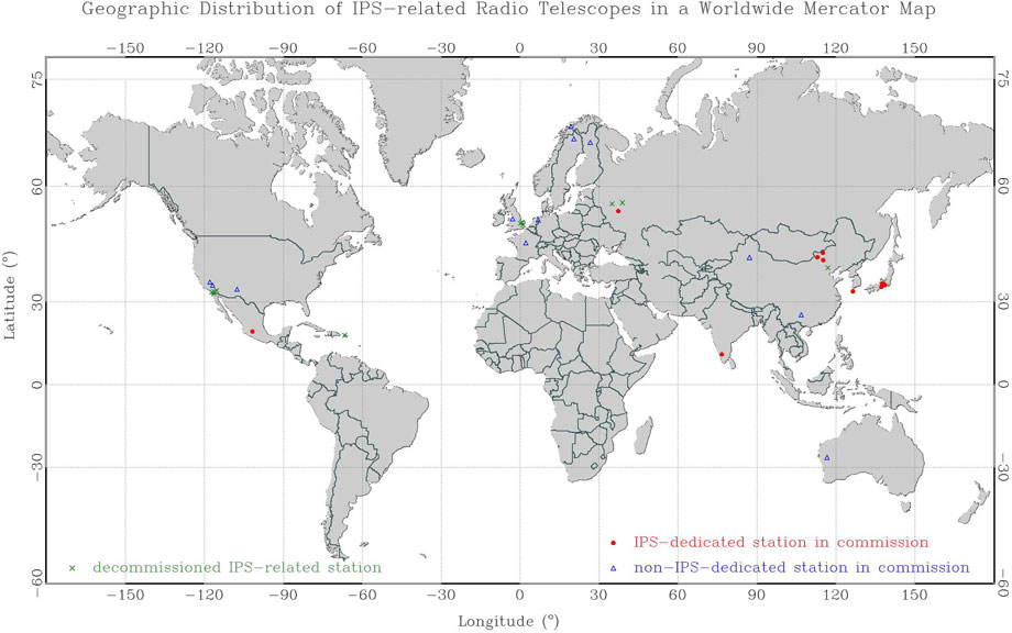
FIGURE 1. Geographic distribution of IPS-related radio telescopes in a worldwide Mercator map.
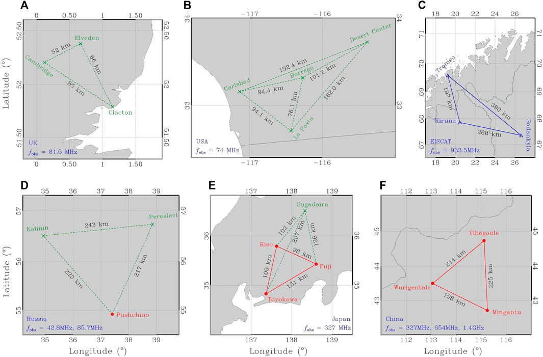
FIGURE 2. Multi-station IPS observations in (A) United Kingdom, (B) United States, (C) northern Europe, (D) Russia, (E) Japan, and (F) China, with the annotated geographic name of each station, baseline length between either two of stations, and observing frequency fobs. The de-commissioned stations and corresponding baselines are annotated in green in each panel.
The current IPS-dedicated radio telescopes include the single-station systems [such as ORT (Manoharan et al., 1995), MEXART (Romero-Hernandez et al., 2015), and BSA LPI (Shishov et al., 2010)] and the multi-site ISEE system (Tokumaru et al., 2011). The ORT has a parabolic cylinder 530 m long in the north-south direction and 30 m wide in the east-west direction (Swarup et al., 1971), which is equipped with a 12−consecutive simultaneous beam system with a separation of ∼ 3 arc-minute between adjacent beams. The BSA LPI telescope at Pushchino has two independent 16-beam systems at frequency of 111 MHz, which is the world’s largest (70,000 m2) currently operating radio array (Shishov et al., 2010). The MEXART consists of 64 × 64 (4,096) full-wavelength dipole antenna array, operating at 140 MHz, with a bandwidth of 2 MHz, occupying about 9,660 square meters (69 m × 140 m) (Mejia-Ambriz et al., 2010). The current ISEE IPS system in commission consists of three antennas at Toyokawa, Fuji, and Kiso. The radio telescope at Toyokawa, called the Solar Wind Imaging Facility Telescope (SWIFT), has the largest aperture among the ISEE IPS system. The SWIFT consists of a pair of asymmetric cylinderical parabolic reflector antennas with an aperture size of 108 m (north-south) by 19 m (east-west) (Tokumaru et al., 2011). A new Chinese IPS-dedicated system under construction consists of one main station and two sub-stations: (1) a parabolic dish antenna with its aperture of 30 m at either sub-station; (2) three cyclindrical parabolic reflector antennas placed side by side at the main station at Ming’antu, each of which is 140 m in north-south direction and 40 m in east-west direction (Wang et al., 2021).
IPS observations have been extensively used to study the solar wind since the first discovery of IPS signals in 1964 by the Cambridge IPS array (Hewish et al., 1964). A comparison with spacecraft observations in the ecliptic is used as a calibration for the IPS observations. According to correlation of IPS and spacecraft plasma density measurements, heliospheric structures can be classified as either corotating or detached from the Sun (Houminer, 1971). The IPS observations have proved to be remarkably sensitive to long lived structures such as corotating interaction region (CIR) (Burnell, 1969; Coles, 1978). In 1970s, the recurrent solar wind streams discovered by IPS observations are statistically correlated with the brightness of the EUV corona in Fe XV (Watanabe et al., 1974). The inverse correlation between the solar wind speed and the magnetic flux expansion factor, proposed by Wang and Sheeley (1990), was substantiated by IPS observations of solar wind speed at different latitudes of the heliosphere during one full solar cycle (Sheeley et al., 1991). The stream interface could be a shear and sliding layer between a fast stream at the high latitude and a slow stream at the ecliptic plane, or a compression layer within the CIR, as the IPS observations detect the velocity gradient and normal scintillation level for the sliding layer, and an intermediate velocity and enhanced scintillation level for the compression layer (Bisi et al., 2010). As revealed from IPS observations, interplanetary CME-driven shocks tend to propagate toward the low-latitude region near the solar equator and the fastest propagation directions tend toward the heliospheric current sheet near 1 AU (Wei and Dryer, 1991; Wei et al., 2005). Using a large-aperture radio telescope, both recurrent CIRs and transient CMEs are readily detected in IPS time-series signals.
The solar wind plasma is collisionless, and waves/turbulence are ubiquitous. Using the solar wind magnetic field data, an effective magnetic Reynolds number is estimated to be about 260,000 ± 20,000 (Weygand et al., 2007). The very large magnetic Reynolds number suggests that large-scale turbulent irregularities should develop, even if the nascent wind were originally smooth and laminar. Because of solar wind density gradients, turbulence in the sub-Alfvénic solar wind is driven by reflection of low-frequency Alfvén waves (Verdini et al., 2009). As the first-ever mission to “touch” the Sun, PSP offers an unprecedented opportunity to characterize the solar wind and the solar energetic particles near their origin. According to PSP’s in situ observation within 0.3 AU, the dominant composition of solar wind turbulence is ascribed to the outward Alfvén mode, and the minor composition is found to be the inward Alfvén mode and the outward fast mode (Zhu et al., 2020). MHD turbulence is always locally imbalanced in creating patches of positive and negative cross-helicities. The conservation of cross-helicity results in a hierarchical structure of MHD turbulence. The slow solar wind is fully mixed by sub-diffusive eddies on time scales corresponding to a 1–2 h crossing time on the Earth; and that solar wind variability on shorter timescales is dominated by turbulent processing, rather than by remnants of variability in the source process at the Sun (DeForest et al., 2015).
The solar wind turbulence is an ensemble of fluctuations with random phases and a broad range of wave vectors. Such fluctuations are manifested in, say, the magnetic field δB, electron number density δn, plasma bulk flow velocity δv. The Elsässer variables for the fluctuating velocity δv and magnetic δB fields are defined as
Here ek is the unit wave vector of k, v the solar wind speed vector, and vp = ω0/|k| the wave phase velocity, where ω0 is the intrinsic wave frequency in the plasma frame. From SB(k), the density fluctuation spectrum Sn(k) can be derived on basis of wave compressibility C(k)
Here n is the mean plasma number density, B magnetic flux density, δn density fluctuation, δB magnetic fluctuation, δE electric fluctuation, Ω proton cycloron frequency, ωp plasma frequency, σ conductivity tensor (Gary, 1986; Harmon and Coles, 2005). The δn, δB, and δE refer to temporal fluctuations at the kinetic scale of Ω, which are estimated to be 32 Hz at 10 R⊙, 1 Hz at 55 R⊙, and 0.1 Hz at 1 AU, respectively (Bale et al., 2016). Whereas, n and B are statistically averaged over a much longer macroscopic scale to be slowly-changing background values. The turbulence amplitude in the corona (Yamauchi et al., 1996) and the heliosphere (Coles and Harmon, 1978) can be measured by IPS observations of electron density spectra. A “turbulent” density spectrum is a direct signature of non-Alfvénic fluctuations such as convected pressure-balance structures (Burlaga et al., 1990) or fast magnetoacoustic waves (Tu and Marsch, 1995; Bruno and Carbone, 2013), because low-frequency Alfvén waves are essentially noncompressive. The near-Sun broadband density spectrum begins with a roughly Kolmogorov power law at large spatial scales of
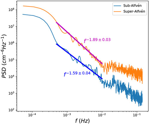
FIGURE 3. Power spectrums for the fluctuating density variance δn in the sub-Alfvénic and super-Alfvénic regions, observed by PSP during its encounter 8 (Zank et al., 2022).
The three-dimensional magnetic fluctuation spectrum SB(k), advected at the solar wind speed v, is measured at a relatively stationary spacecraft as temporal turbulence data SBsc(f). The one-dimensional frequency spectrum measured by spacecraft is termed “spacecraft magnetic spectrum” (Harmon and Coles, 2005). Using Taylor’s hypothesis, the measured magnetic frequency spectrum can be interpreted as mapping of the turbulence wave-number into the stationary spacecraft frame.
Here the x-direction is along the solar wind velocity vector. Taylor’s hypothesis assumes that when the turbulent fluctuations are advected with a speed v that is much higher than the typical fluctuation speed δv(v ≫ δv), the time (τ) and the spatial (r) lags of the measured structures are connected as r = vτ. The frozen-in approximation is not strictly valid inside the Alfvén surface, where PSP is periodically scheduled to explore.
In-situ measurements of magnetic field fluctuation of interplanetary solar wind have substantiated a power law spectrum as |δB(f)|2 ≈ f−α. The solar wind turbulence in an inertial range is similar to the classical Kolmogorov picture of fluid turbulence, and the spectral index α is approximately 5/3 (Leamon et al., 1998). Then, the Kolmogorov dissipation rate Qkol can be evaluated from velocity fluctuation
Where
Further, Qkol can be quantitatively incorporated as an observation-constrained empirical term in numerical MHD models of Alfvén wave turbulence-driven solar wind to generate the global distribution of solar wind MHD parameters from the inner corona to 1 AU (e.g., Li et al., 2004).
Consider a planar layer of turbulent plasma with its inherent density fluctuations δn(r), a planar radio wave propagating through the turbulent layer would experience accompanying phase fluctuations δϕ(r) = re λ δn(r) Δz (Bastian, 1994). Here, re is the classical electron radius, λ the radiation wavelength, Δz the depth of turbulent plasma layer.
The planar turbulent layer can be consider as an infinitely thin “two-dimensional phase-changing screen” ϕ(x, y) at z = 0, whose statistical properties are independent of x, y, and time t. A mean-squared phase
With ϱ(0, 0) = 1 and
The first derivative of ϱ(r) vanishes at the origin, under the reasonable assumptions that q0x and q0y are finite and that ϕ2(qx, qy) is an even function. The two-dimensional (2D) ACF may be anisotropic and have different correlation lengths along the x − and y − directions. Here, the 2D “correlation lengths” are defined by
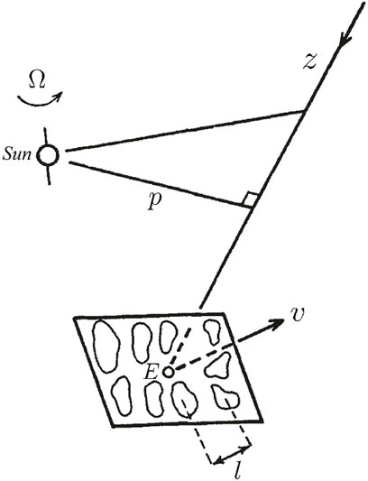
FIGURE 4. Geometry of the IPS diffraction pattern observed at the Earth due to turbulent solar wind irregularities (Hewish et al., 1964).
A length z0 ≡ k a2 is defined as the “Fresnel distance” for diffraction from turbules of size a. Then, another length l0 ≡ z0/ϕ0 ≡ k a2/ϕ0 is defined as the “typical focal length”. The “thin phase screen” theory can be extended to the regime where the rms phase fluctuations are large and distances to the screen z are comparable with typical focal lengths l0 (Salpeter, 1967). Supposing that a plasma slab of thickness Δz depicted in Figure 4 is comparable with the distance of closest approach to the Sun, the triple inequality of λ ≪ a ≪Δz ≪ z generally holds. The phase along one radio ray path is delayed due to the fluctuating refractive index. Also, the ray path is lengthened due to refraction. The “thin phase-screen” approximation is still justified when the two inequilities of z0 ≫Δz and l0 ≫Δz hold, for any ϕ0 and z (Salpeter, 1967).
For an extended radio source with its angular size θ0, the brightness is usually supposed to have a Gaussian distribution
As δI is the fluctuation in intensity I about its mean
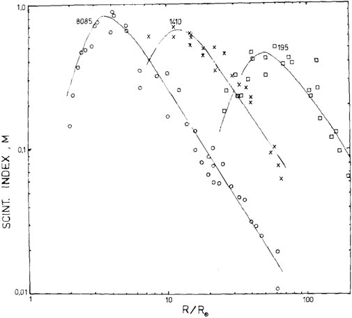
FIGURE 5. Heliocentric variances of radio scintillation indices at three different frequencies of 8,085, 1,410, and 195 MHz (Coles, 1978).
The space and time correlation of intensity fluctuations is evaluated by equation
The IPS model for the local intensity modulation of radio waves makes use of a Born approximation to the general weak scattering theory (Tatarskii et al., 1993). The spatial fluctuation of the local density irregularities is conveyed by the ambient solar wind flow, and consequently introduces a scintillation pattern in the (x, y) plane perpendicular to the IPS ray-path along the z direction. Here (x, y, z) is a Cartesian coordinate system centred on the Earth. The intensity PδI in a total spectrum of the spatial wave vector q is merely a linear superposition of all contributions from every thin scattering layer along the IPS ray-path connecting the Earth to an extragalactic radio source, as described by PδI = ∫δPδI (q, z) dz. The two-dimensional spatial wave vector q can be resolved into (qx, qy) components in the reference of IPS ray-path or (q‖, q⊥) components in the reference of local magnetic field. The absolute value of spatial wavenumber q is evaluated as
Here, w(q) is a weighting factor at spatial wave vector q, the plasma number density fluctuation δn, the classic electron radius re = 2.82 × 10⁻⁵ m, the Fresnel radius rF = (λ z)1/2, the spectral exponent α, and the axial ratio of anisotropy degree AR (Coles and Harmon, 1989; Klinglesmith, 1997; Xiong et al., 2011). When λ = 1 m, and z = 1 AU (1.5 × 10¹¹ m), the Fresnel radius is about 387 km. The cylindrically-symmetric coordinate system (q‖, q⊥) with its axis along the local magnetic field is transferred from the coordinate system (x, y, z) defined with respect to the IPS ray-path. As the variation of δn along the IPS ray-path z is not known a priori, it is a common practice in IPS studies to assume some empirical δn variances such as δn ∝ n (Houminer and Hewish, 1972) and δn ∝ rPWRnPWN (Asai et al., 1998). Here, r is the heliocentric distance, PWR a power of radial falloff, and PWN the power of electron density. The parameters of PWR and PWN are determined via best fit of IPS data over one interval chosen. Particularly, the term Fdiff is a high-pass Fresnel filter with its Fresnel radius rF. Such a radius rF determines the maximum scale of the irregularities, at which the amplitude fluctuation can be received at the Earth.
Using solar wind velocity to relate the temporal and spatial fluctuations, the one-dimensional (1D) temporal power spectrum Pf recorded at the Earth can be calculated as an integral of multiple 2D “phase screen” δPδI (qx, qy, z) along the z −axis. The spatial spectrum of intensity δPδI (qx, qy, z) carried by an anti-sunward solar wind speed v, which is drifted across an IPS ray-path with its intersection angle 90° − θ. Only the speed component perpendicular to the IPS ray-path Vdrift = |v|⋅ cos θ is detectable by a terrestrial radio antenna. Vdrift is the solar wind velocity projected on to the “phase screen” perpendicular to the z−axis. As depicted in Figure 6, the geometry factor cos θ varies along the entire IPS ray-path. Supposing Vdrift in the “phase screen” is along x−axis, the temporal frequency of IPS signal f is derived as f = qxVdrift/(2 π), and the temporal IPS spectrum P(f) is derived from the following equations:
for an infinitely thin “phase screen” δz at point p.
for an finite-depth “phase screen” astride point p.
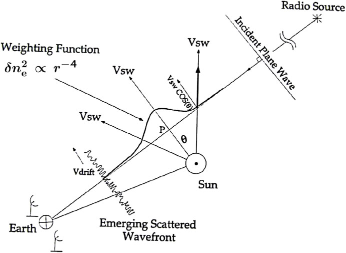
FIGURE 6. Geometry factor cos θ varies along the entire IPS ray-path (Grall, 1995).
Accordingly, the scintillation index m is related to small-scale density variations along the z−axis by the equation
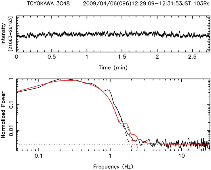
FIGURE 7. A typical time-series of IPS signals from radio source 3C48 recorded by SWIFT at Toyokawa, with its normalized power spectral fitting denoted as red lines (Tokumaru et al., 2011).
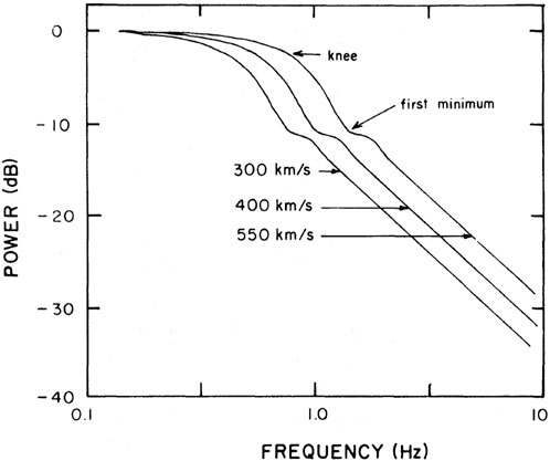
FIGURE 8. An example of power spectral fitting of ORT IPS data for various solar wind speeds (Manoharan and Ananthakrishnan, 1990).
The IPS signals can be simultaneously recorded at multiple stations, as shown in Figure 2. The separation of two receiving antennas at the order of 200 km provides an appropriate range of baselines and allows an accurate determination of the spatial properties of the drifting pattern. Because of the Earth’s rotation, the baseline projected onto the celestial sphere describes an ellipse and a radio source can be observed with a baseline heavily fore-shortened (Bourgois et al., 1985). For instance, a triangular network of observing sites at Serpukhov, Pereslavl, and Kalinin in Russia was built to record IPS signals from the same radio source (Figure 9). The multi-station scintillation method of measuring the solar wind velocity has been very accurate, particularly near the Sun and at high heliographic latitudes (Kojima et al., 2013). The nearly frozen-in diffraction pattern δPδI(qx, qy, z) can be sequentially received by two radio stations separated by a baseline s. If the baseline s is approximately parallel to the drifting direction Vdrift of interplanetary density irregularities, the scintillation patterns at the two telescopes will be correlated with some time lag τ. Specifically, the spatial-to-temporal conversion is merely a cut in the spatial correlation function along the direction of (s − Vdrift ⋅ τ). When the baseline s is zero, the cross-correlation function (CCF) between two stations is degenerated to the ACF, which always has a component of uncorrelated white noise at zero lag. For a single scattering layer, the CCF is simply derived by shifting the ACF at a time lag |s|/|Vdrift|. Inversely, the drifting speed |Vdrift| can be inferred from the time lag τ, which is the manifestation of flow speed of local density irregularities. Thus, the vector velocity Vdrift is calculated from three time delays identified along each baseline of joint three-station measurements. However, the calculated flow speed Vdrift is a weighted integral along one IPS ray-path. The apparent drifting speed Vdrift could be biased from the local solar wind velocity v(z).
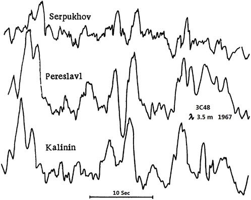
FIGURE 9. An example of simultaneous three-station recording of IPS signals from radio source 3C48 in 1967 (Vitkevich and Vlasov, 1970).
In the Born approximation, the CCF along a baseline s can be described by the following equation.
The velocity v(z) probably has two random components: (1) one parallel component expected from the radial variations of solar wind speed in the scattering region; (2) one perpendicular component anticipated from radially propagating Alfvén waves. These random components result in an apparent spread of pattern-drifting speed around some mean large-scale bulk-flow speed. Little and Ekers (1971) proposed that the drifting and changing scintillation pattern can be modelled as an ensemble of frozen-in patterns, each having a spatial ACF C(s, 0) and a pattern speed v. Then, IPS CCF can be integrated over a probability density function (PDF) p(v) of the form
A prescription of p(v) can be uniform (Grall et al., 1996) or Gaussian (Kojima et al., 2013). The observed CCF C(s, τ) are usually normalized by the square root of the product of the two ACFs at zero lag τ = 0. IPS velocities are computed by making model fits to the shape of the normalized CCF. A long baseline can improve the ability to resolve streams of different velocities (Grall et al., 1996; Breen et al., 2006; 2008; Bisi et al., 2010), provided that the time interval is long enough to derive well-defined scintillation spectra, when the observing geometry is suitable for CCF analysis. Herein, though the baseline between Multi-Element Radio Linked Interferometer Network (MERLIN) and EISCAT network is extremely long to be 2,000 km, correlation between the scintillation patterns observed on 15 May 2002 was still significant (Breen et al., 2006). When an IPS ray-path traverses through both fast and slow solar wind streams, the delay−CCF profile measured by widely separated stations such as EISCAT radar has two clearly separated peaks: one narrow peak at a short delay, the other broad peak at a large delay. If measured by closely spaced stations such as ISEE radio array in Japan, only one peak exists in the delay−CCF profile. As the baseline between two stations is gradually shortened, two distinct peaks would overlap and merge into one compound peak. Multi-streams along an IPS ray-path produce a skewed CCF, but the degree of this skewness depends on the baseline length: a longer baseline produce a stronger skewness (Kojima et al., 2013). The CCF analyses between more closely spaced stations is used to estimate an intermediate velocity perpendicular to one IPS ray-path, which is averaged between multiple solar wind streams cut by the IPS ray-path.
Using a long baseline to de-convolve the LOS integration of CCF measurements, multiple solar wind streams are discernible from the measured delay−CCF profile. As shown in Figure 10, double-peaked CCFs are found from EISCAT observation of south polar solar wind, whose baseline was 240 km radial and 3 km tangential. The fast and slow wind speeds are inferred to be 500 and 777 km s−1 on basis of one model fit of the delay−CCF profile (Grall et al., 1996). Various IPS observations using EISCAT, MERLIN, Very Long Baseline Array (VLBA) antennas substantiate that the acceleration of polar solar wind is almost completed within a heliocentric distance of 10 R⊙ (Grall et al., 1996; Klinglesmith, 1997). However, the velocities of the near-Sun solar wind derived from IPS measurements have a large velocity spread. This large velocity spread, mostly aligned along the radial direction within 20 R⊙, is considered to be caused by the Alfvén-wave motion (Harmon and Coles, 2005; Kojima et al., 2013). The dominant contributor to the velocity spread is LOS projection effects rather than changes in wave dispersion near the ion cyclotron frequency (Harmon and Coles, 2005). As the amplitude of Alfvén turbulence is much smaller in the interplanetary space compared with the inner solar corona, IPS speed is likely to be close to the bulk plasma flow speed, at least in the slow solar wind (Klinglesmith, 1997).
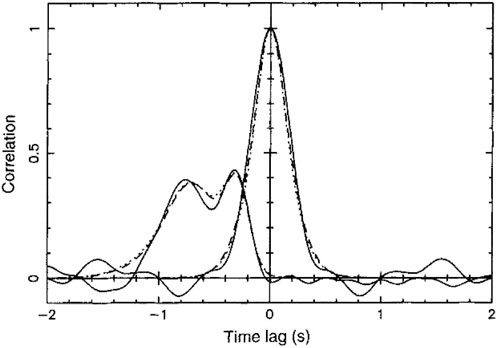
FIGURE 10. Intensity correlation functions from EISCAT observation of radio source 0323 + 055 at −52° helio-latitude on 28 April 1994 (Grall et al., 1996).
The basic solar wind parameters include the mean velocity, random velocity, spatial anisotropy, and micro-turbulence spectrum. Near the Sun, spatial structure is quite anisotropic (Dennison and Blesing, 1972) and the solar wind speed has an important random component (Little and Ekers, 1971). The random velocity is insignificant at distances greater than 40 R⊙, but increases rapidly with decreasing distance, approaching the mean velocity by 20 R⊙ (Scott et al., 1983a). The solar wind velocity can be recursively estimated by fitting the temporal power spectra observed with a single antenna, or straightforwardly calculated by using the time delays between three pairs of radio antennas. A comparison between single-station and three-station solar wind measurements (Manoharan and Ananthakrishnan, 1990; Mejia-Ambriz et al., 2015; Chashei et al., 2021) generally showed good agreement within the error estimates. For instance, using nearly simultaneous IPS observations by both BSA LPI and ISEE radio telescopes, Chashei et al. (2021) found the correlation between the daily speed estimates from the compact source 3C48 is 50% during 6 years from 2014 to 2019. All the IPS records studied by Shishov et al. (2010) were selected by the range of radio source elongations between 25° and 60°, which corresponds to heliocentric distances of LOS p −points within the range of 0.4 and 0.8 AU. However, the single-station model-fitting process was found to be difficult for solar distance less than 40 R⊙, because in this range neither random velocity nor spatial anisotropy can be neglected (Scott et al., 1983a). The multi-station joint observation can separate the similar effects of random velocity and anisotropy. The models developed with the multi-station data can be extrapolated to the entire class of single station observations (Scott et al., 1983a). The solar wind speed vector derived from the multi-station cross-correlation analyses is valid for any strength of scattering and is independent of the existence of turbulence in the velocity field (Bourgois et al., 1985; Chashei et al., 2021). A comparison between the single-station and multi-station methods of velocity estimation is essential to examine a possible systematic bias between them and thus to improve the accuracy of IPS observation (Tokumaru et al., 2011), which is routinely performed for the ISEE IPS observations.
The 3D solar wind flows are remotely sampled at multiple discrete IPS ray-paths over a large portion of Sun-centered sky map. To optimize the use of IPS observations and produce 3D global heliospheric representations, two iterative CAT models were separately developed in late 1990s (Jackson et al., 1998; Kojima et al., 1998) that fit IPS observations of drifting speed Vdrift and scintillation factor g to a kinematic solar wind model to provide 3D velocities and densities. The general flowchart for numerical IPS-CAT models is plotted in Figure 11, with the same notations as used in the text of Jackson et al. (2010c). The subscripts j and k are used when physical quantities such as density n and speed v refer to discrete Nθ × Nφ grids on a 2D reference sphere. The spatial resolution of current CAT models along latitude and longitude directions is typically at 5°–10° (Hayashi et al., 2003; Jackson and Hick, 2004; Hayashi et al., 2016). The reference sphere, also called source surface, is usually set at the super-Alfvénic region, i.e., rref = 30Rs. Because the realistic solar wind flows are already accelerated at the inner boundary of rref, the complicated mechanisms governing tran-Alfvénic acceleration and heating of solar wind flows are absent within the simulation domain of IPS-CAT models. An initial prescription of the inner boundary condition can be arbitrary, as a unique solution of solar wind speed distribution on the inner boundary is gradually converged as a result of repeated perturbation of radial speed δvr,j,k at the boundary mesh.
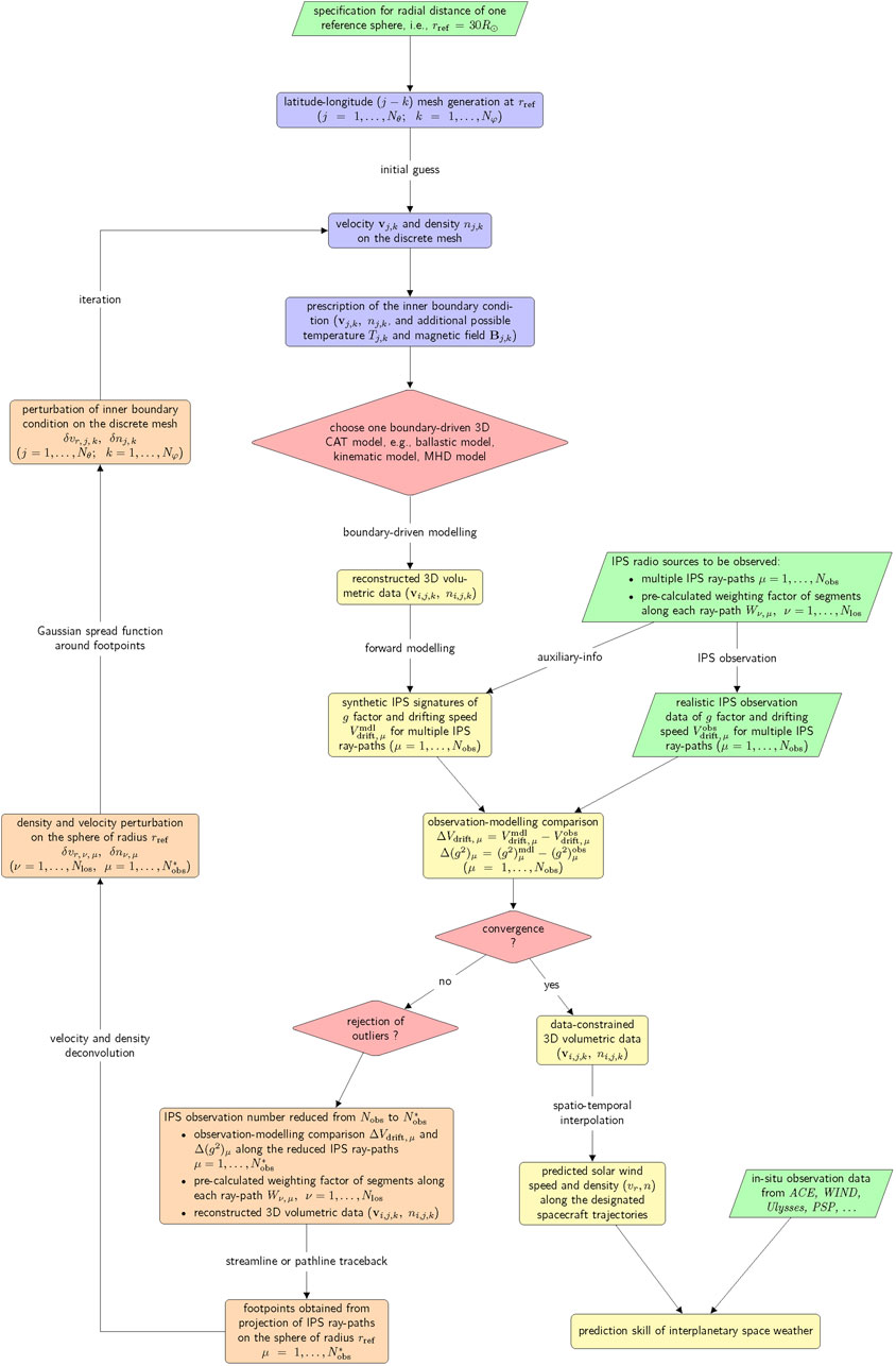
FIGURE 11. The general flowchart for numerical CAT models of the inner heliosphere constrained by IPS data.
The essence of IPS-based CAT models is an automatically iterative procedure modifying the solar wind velocity distribution on an inner boundary sphere. The boundary-driven 3D CAT models can be ballistic, kinematic, or magneto-hydrodynamical according to physical description of solar wind flows. For a ballistic model, the solar wind plasma velocity is assumed constant along the streamlines (Kojima et al., 1998). For a kinematic model, the momentum and mass are conserved to describe the collision and merge of different solar wind plasma parcels emanating from the inner boundary (Jackson et al., 1998). For an MHD model, nonlinear MHD processes are self-consistently simulated to address very complicated interplanetary dynamics from near the Sun to well beyond 1 AU, such as shock formation. The mathematical treatment of the solar wind flows in IPS-CAT models is increasingly sophisticated from the ballistic model to the kinematic model, and then to the MHD model. Using any of these IPS-CAT models, 3D volumetric data of speed vi,j,k is numerically reconstructed.
The simulation of IPS velocity measurement
where z is the position vector of a point on the ray-path at the distance z from Earth. The weighting factor ϖ(z) is calculated as an integral over spatial wave vector q, i.e.,
With the 3D distribution of vi,j,k within the simulation domain, IPS data made at various heliocentric distances and times are traced back along the streamlines to the source positions on the inner boundary. In Figure 11, subscript μ is used to identify a LOS while ν refers to a segment at a certain distance from the observer along the LOS. On the footpoints backwards mapped from each IPS ray-path, radial speed is perturbed to be δvr,μ,ν for ν = 1, 2, …, Nlos and
IPS data-constrained numerical CAT 3D models can reconstruct the transient CME structures and their ambient large-scale solar wind flows. The Carrington maps of velocity and density at the inner boundary are smoothed each iteration using a 2D Gaussian spatial filter and a 1D Gaussian temporal filter (Jackson et al., 2010c). Such a temporal filter on the inner boundary is not used to reconstruct the global structures of corotating solar wind. For a corotating IPS-CAT model, the global solar wind is assumed to be slowly evolving in time during one Carrington rotation. The absolute density scale of the solution cannot be determined from the tomographic reconstruction itself, because g−level is a proxy for the solar wind density variance. The averaged scale of reconstructed density is externally calibrated according to in situ measurements near the Earth. For the UCSD kinematic IPS-CAT model, g−levels can be replaced or augmented by heliospheric Thomson-scattering intensity as measured by the Solar Mass Ejection Imager in a polar orbit around the Earth (Jackson et al., 2010c). As shown in Figure 12A, IPS scintillation indices calculated from the 3D density distribution of numerical MHD simulations are useful in denoting CME propagation direction on the plane of sky (Iwai et al., 2021). As shown in Figure 12B, the 3D numerical solution of MHD IPS-CAT model has been demonstrated to be able to simulate the Archimedean spiral structure of the solar wind on the equatorial plane, and match the in situ near-Earth and/or Ulysses observation data during one Carrington rotation period (Hayashi et al., 2016). The 3D global structures of interplanetary disturbances, daily reconstructed from the UCSD kinematic IPS-CAT model, are shown in the website of https://ips.ucsd.edu/ for the purpose of real-time space weather forecast. One of the data products generated from the tomographic reconstruction is the large-scale distribution of 3D density structures shown in Figure 12C (Jackson and Hick, 2004).
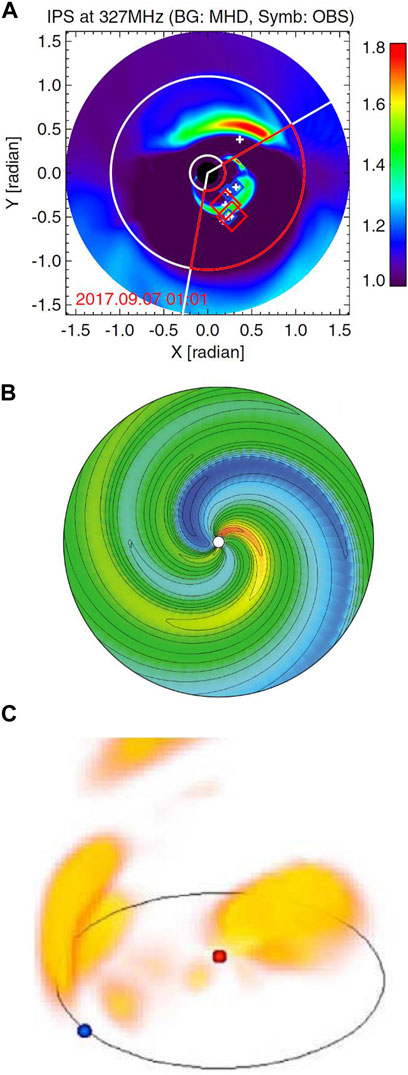
FIGURE 12. Some IPS-related numerical 3D models for space weather modelling: (A) multi-source observations of IPS g−value and their comparison with the SUSANOO-CME MHD simulation (Iwai et al., 2021), (B) radial speed of solar wind on the equatorial plane derived by the MHD-IPS Hayashi model (Hayashi et al., 2016), (C) 3D distribution of the corotating component of plasma density in the inner heliosphere during Carrington rotation 1884 reconstructed by the UCSD IPS-CAT model (Jackson and Hick, 2004). In panel (A), the cross symbols represent all observed radio sources, and the diamond ones indicate radio sources with the g-values of g > 2 (red), 1.5 < g < 2.0 (green), and 1.2 < g < 1.5 (blue). In panel (B), blue, yellow, and orange colors approximately represent radial speed of 700, 500, and 300 km s−1, respectively. In panel (C), the density is normalized by the removal of its r−2 dependence on heliocentric distance r.
Regarding multiple iteration steps, there is a major difference between the UCSD time-dependent kinematic IPS-CAT model and other MHD IPS-CAT models. The former goes through a Carrington rotation or any time period in a single “time-dependent” run (or iteration). In other words, each iteration is a time-dependent simulation by itself. On the other hand, the latter performstomographic iteration for a steady state simulation at a certain time cadence (typically 1 day), and then a time-dependent MHD simulation is performed afterwards using the iteratively constrained boundary conditions. Streamlines are imaginary lines that representthe direction of the flowing fluid at a certain point in time. Only in a steady flow are streamlines identical to pathlines, which are defined to be flow paths that the fluid particles take while flowing. The above-mentioned difference between different tomography models is essentially ascribed to the inconsistency between pathlines (also called trajectories) and streamlines in an unstable flow.
The UCSD kinematic IPS-CAT model can accurately reproduce the general large-scale 3D structure of the solar wind density and speed in the inner heliosphere, and even smaller-scale fluctuations at 6-h cadence at Earth (Jackson et al., 2015; Jackson et al., 2020). Obviously, all the IPS ray-paths converge at Earth, so near-Earth space in the IPS-CAT model is always very well constrained by IPS data. The in situ velocity measurements at the first Sun-Earth Lagrangian point (L1), such as near-real time Advanced Composition Explorer (ACE) data, are further included into the UCSD time-dependent tomography to constrain the iterated results (Jackson et al., 2010b). As a result, the current “L1-data constrained” kinematic IPS tomography performs remarkably at Earth, with Pearson correlations typically above 0.9. In addition, the 3D solar wind velocity reconstructed from the UCSD kinematic modelling can be used to carry and extend the solar magnetic field lines, described by the current sheet source surface model (Zhao and Hoeksema, 1995), out to the edge of the global boundary considered by the IPS analysis (Jackson et al., 2012). Such IPS-aided information about disturbed solar wind structures in three dimensions is valuable in interpreting in situ observations from interplanetary spacecraft.
The inner boundary conditions provided by the UCSD time-dependent tomography have been used to drive multiple numerical MHD models, such as MS-FLUKSS model (Kim et al., 2014), ENLIL model (Jackson et al., 2010a), Alfvén Wave Solar atmosphere Model (AWSoM) (Sachdeva et al., 2019). An ad hoc adjustment of the inner boundary values in the MS-FLUKSS MHD model could deliver more comparable results at Earth, but diverges considerably from the UCSD kinematic IPS-CAT model below 100 R⊙(Kim et al., 2014). Sachdeva et al. (2019) compared the AWSoM MHD model with the UCSD kinematic IPS tomography at 20, 100, and 215 R⊙, and found reasonable agreements at 100 and 215 R⊙ and a 20–30% discrepancy at 20 R⊙; Jian et al. (2015) compared all the coronal and heliospheric model combinations (including MHD models) installed at the NASA Community Coordinated Modeling Center (CCMC) and found that the kinematic IPS tomography correlated best with the solar wind speed and density measured at Earth. On the other hand, when the same CCMC models were compared with Ulysses data during the fast latitudinal scan in 2007, the kinematic IPS tomography deviated significantly when Ulysses was away from Earth and the ecliptic plane (Jian et al., 2016), confirming what Kim et al. (2014) showed earlier. The performance drawback of the UCSD kinematic IPS-CAT model at Ulysses orbit is owing to two reasons that “the numbers of IPS signals are limited out of the ecliptic plane at present” and “IPS observations over the north and south ecliptic poles are generally obtained close to the solar surface” (Jian et al., 2016). The outstanding mystery of the solar wind acceleration nearer the Sun is insufficiently addressed in the mathematical descriptions of current IPS-CAT models, which results in the degenerated performance of kinematic IPS-CAT model at Ulysses orbit (Jian et al., 2016) and the noticeable prediction discrepancy between different IPS-CAT models at 20 R⊙ (Sachdeva et al., 2019). The differences between the IPS kinematic-model data-fitting procedure and the current 3D MHD modeling techniques provide interesting insights into the physical principles governing the expulsion of CMEs as well as expectations and limitations of various IPS-CAT models (e.g., Jackson et al., 2015; Yu et al., 2015).
The intensity variance of IPS signals on the time-scale of 0.1–10 s for the micro-scale density irregularities, with a characteristic scale of tens to a few hundred of kilometers. The sensitivity of radio telescope is characterized as system noise temperature Tsys, effective aperture area Ae, and minimum detectable flux density ΔSmin. A high-sensitivity radio system to observe celestial compact radio sources is desired, because the flux of IPS signals received at Earth are generally faint to be less than 1 Jansky. Due to increasing of radio telescope sensitivity, much more fainter radio sources are found to have the IPS phenomena. However, man-made radio emissions in all frequency bands are increasingly causing serious interference signals for most of radio astronomical observatories in the world. Under the guidance of International Telecommunication Union, radio frequency spectra are painstakingly parcelled out between radio-based applications such as personal communications, satellite broadcasting, GPS and amateur radio, and the sciences of radio astronomy, Earth exploration and deep-space research. The key bands of VHF and UHF radio spectra widely used in IPS observations should be carefully protected by the local administrative regulations. As shown in Figure 2, the observing frequencies for the current IPS-dedicated radio telescopes are 327 MHz in India and Japan, 111 MHz in Russia, 140 MHz in Mexico.
The numerical IPS-CAT models have been proved to be capable of reconstructing 3D large-scale velocity and density structures in the inner heliosphere. Such a 3D reconstruction of interplanetary structures is of great interest for the space weather prediction community. Since the routine IPS observations at the ISEE in 1999, a near real-time prediction analysis system on basis of UCSD kinematic IPS-CAT model have been operated and developed for over two decades to provide heliospheric solar wind speed and density at Earth (Jackson et al., 2010b) and at Mars (Jackson et al., 2007). The construction of SWIFT at Toyokawa in the late 2000s significantly upgraded the overall sensitivity of the ISEE IPS system, and achieved a finer resolution in the CAT reconstruction from those IPS data (Tokumaru et al., 2011; Hayashi et al., 2016). The time cadence interval used by the UCSD IPS-CAT modelling is relatively short in comparison with that of a solar rotation, i.e., about 1 day for ISEE IPS data (Jackson et al., 2015). The spatial and temporal resolutions of IPS-CAT models are essentially constrained by the number of available IPS ray-paths.
The insufficient sampling of the inner heliosphere provided by the existing observations of IPS can be ascribed to several reasons including limited sky coverage in declination and hour-angle, insufficient sensitivity, limitations posed by weather and geographic locations, and slow slew rate of antenna beams (Oberoi and Benkevitch, 2010). For instance, the SWIFT antenna at Toyokawa forms a single beam in the local meridian, steerable between 60°S and 30°N with respect to the zenith (Tokumaru et al., 2011), which results in sparse polar coverage, especially in the southern hemisphere. The solar wind speeds and scintillation levels have been basically determined on a daily basis between April and December from ISEE IPS observations. However, the ISEE IPS data are unavailable in winter owing to snow at the observatories (Tokumaru et al., 2021), and has noticeable coverage gaps in certain parts of the sky because of the unevenly scattered IPS sources. An extensive gap in the ISEE IPS tomography map data due to the above-mentioned reasons had better be filled by an analytic Legendre-polynomial formula for the latitudinal profiles of the yearly filtered solar wind speed (Porowski et al., 2022). As IPS observations are usually taken around the time of meridian transit for each radio source, daily meridian scan observations of the sky map around the Sun can be sequentially made at multiple IPS stations located at different geo-longitudes. The coordinated observation of multiple IPS-dedicated stations distributed at different time zones on the Earth is highly desired to improve the routine prediction performance of IPS-based tomographic reconstruction.
The Worldwide IPS Stations (WIPSS) Network aims to bring together the worldwide real-time capable IPS observatories with well-developed and tested analysis techniques (Bisi et al., 2019). Now, the real-time internet access to the original IPS observation data is only provided by the ISEE IPS system among these IPS-dedicated radio telescopes. Other IPS-dedicated radio telescopes at Ooty and Pushchino have accumulated a huge volume of IPS data since their operations in the 1970s. The Ooty radio telescope is unique for its long axis of parabolic cylinder reflector being parallel to the Earth’s rotation axis. Using such an equatorial mount, a celestial radio source can be tracked for about 10 h by the mechanical rotation of the cylinder in the east-west direction (Manoharan, 2010). Some non IPS-dedicated radio telescopes such as EISCAT (Bourgois et al., 1985), LOFAR (Fallows et al., 2016), and MWA (Morgan et al., 2018) have been intermittently used to study IPS phenomena. The southern-biased FOV of MWA provides a good complement to the northern-biased FOV of other telescopes located at the northern hemisphere of the Earth. The LOFAR4SW project, implemented under the European Horizon 2020 programme as a design study, was to develop an upgrade to the existing LOFAR infrastructure so that it would be possible to use the instrument’s capabilities for space weather purposes (Bisi et al., 2020; Carley et al., 2020). In addition, the new Chinese IPS-dedicated radio telescopes under construction in northern China will join the WIPSS network for the international space weather service. The daily observed radio sources are estimated to be nearly 100 by SWIFT (Iwai et al., 2021), 500 by MEXART (Mejia-Ambriz et al., 2010), and several thousand by ORT (Manoharan et al., 2017) and BSA LPI (Chashei et al., 2021). Different IPS techniques (single-site versus multi-site) and analysis procedures followed at different observatories need to be cross-calibrated against one another to yield consistent results (Oberoi and Benkevitch, 2010). Jackson et al. (2023) demonstrated that both spatial and temporal coverage of UCSD kinematic CAT model can be significantly increased with more IPS data input from ISEE, LOFAR, and BSA LPI within the WIPSS network groups.
IPS is the phenomenon of random fluctuations in the intensity of distant compact object, smaller than an arc-second, induced by the ubiquitous inhomogeneous structures in the turbulent solar wind. The radio signal from a distant compact radio source is scattered by the density inhomogeneities of the solar wind on the order of 100 km. A diffraction pattern of radio intensity fluctuations arises from the interference between any pair of incident plane waves. The spatial correlation length of density inhomogeneities and the Fresnel radius of radio diffraction are two key parameters in determining the scintillation pattern. In weak scattering, a “2D phase-chaning screen” scenario is justified on the basis of the Born approximation. The diffractive contribution of the scattered signal is quantified as a Fresnel filter in weak-scattering theory. In strong scattering, scintillation index decreases because intensity variation interferes or cancels each other within the observation frequency band. A typical power spectra of IPS signals recorded at a single station is flat at low frequencies, then has a sudden drop over the Fresnel knee. Using a nonlinear spectral-fitting method, the IPS power spectra around the knee is analyzed to infer solar wind velocity, radio source size, and turbulence spectral index. The intensity diffraction pattern that transported away from the Sun by the solar wind can be measured and correlated between multiple radio stations on the Earth. Two simultaneous IPS time series from separate stations can be cross-correlated to determine the solar wind speed from time delay. Using three stations for IPS allows the solar wind velocity vector to be determined to a high degree of accuracy. Therefore, IPS serves as an effective tool for remote sensing of the inner heliosphere, determining the flow speed and turbulence amplitude associated with either undisturbed solar wind or transients, such as CMEs.
The global 3D distribution of solar wind speed and density can be determined by current IPS-based numerical CAT models. The simulation domain of those IPS-CAT models are generally prescribed beyond the Alfvén surface of solar wind flows. Tokumaru et al. (2021) compared solar wind speeds derived from the IPS-CAT analysis with in situ observations conducted by the near-Earth and Ulysses spacecraft, and found that the discrepancy between the IPS and in situ observations can be improved by changing the power index of the empirical relation between the solar wind speed v and density fluctuations δne. The real-time IPS predictions often suffer reduced performance since they are limited to the data available only up to the time when the prediction is made (Jackson et al., 2015; Jackson et al., 2020; Jackson et al., 2023). With a large number of IPS radio sources to be observed by the WIPSS network on a regular daily basis, IPS-CAT models can be fully exploited to map and predict the structure and motion of major disturbances in the inner heliosphere. The potential synergy between the above-mentioned IPS-capable radio telescopes on the Earth, complemented with other ground-based and spaceborne instruments, would enable the simultaneous exploration and scientific understanding of solar wind dynamics and structures in three dimensions, thereby facilitating major breakthroughs in the interplanetary space weather prediction.
MX was responsible for the organization of this article, contributed to all sections, and wrote the initial manuscript version. KY provided the important insights on how to design figures 2 and 11, and made major contributions to the revision of sections 2. All authors contributed to the initial concept, read and revised the paper, approved the final version.
This work was jointly supported by the National Natural Science Foundation of China (41874205, 42074208, 42241118, 42030204, 41974200, 42174201, U2031134, 12003049, 12203056), National Key R&D Program of China (2021YFA1600500, 2021YFA1600503), the Specialized Research Fund for State Key Laboratories of China, the Meridian Space Weather Monitoring Project in China.
We sincerely thank both reviewers for their constructive comments and suggestions.
The authors declare that the research was conducted in the absence of any commercial or financial relationships that could be construed as a potential conflict of interest.
All claims expressed in this article are solely those of the authors and do not necessarily represent those of their affiliated organizations, or those of the publisher, the editors and the reviewers. Any product that may be evaluated in this article, or claim that may be made by its manufacturer, is not guaranteed or endorsed by the publisher.
Abe Pacini, A. (2020). “The Arecibo NOON (coroNa tO sOlar wiNd) project,” in AGU fall meeting abstracts, 2020, SH041–09.
Armstrong, J. W., and Coles, W. A. (1972). Analysis of three-station interplanetary scintillation. J. Geophys. Res. Space Phys.77, 4602–4610. doi:10.1029/JA077i025p04602
Asai, K., Kojima, M., Tokumaru, M., Yokobe, A., Jackson, B. V., Hick, P. L., et al. (1998). Heliospheric tomography using interplanetary scintillation observations 3. Correlation between speed and electron density fluctuations in the solar wind. J. Geophys. Res. Space Phys.103, 1991–2001. doi:10.1029/97JA02750
Bale, S. D., Goetz, K., Harvey, P. R., Turin, P., Bonnell, J. W., Dudok de Wit, T., et al. (2016). The FIELDS instrument suite for solar Probe plus. Measuring the coronal plasma and magnetic field, plasma waves and turbulence, and radio signatures of solar transients. Space Sci. Rev.204, 49–82. doi:10.1007/s11214-016-0244-5
Barnes, A. (1979). “Hydromagnetic waves and turbulence in the solar wind,”. Solar system plasma physics. E. N. Parker, C. F. Kennel, and L. J. Lanzerotti, 1, 249–319.
Bastian, T. S. (1994). Angular scattering of solar radio emission by coronal turbulence. Astrophys. J.426, 774. doi:10.1086/174114
Bisi, M. M., Fallows, R. A., Breen, A. R., and O’Neill, I. J. (2010). Interplanetary scintillation observations of stream interaction regions in the solar wind. Sol. Phys.261, 149–172. doi:10.1007/s11207-009-9471-1
Bisi, M. M., Jackson, B. V., Gonzalez-Esparza, A., Aguilar-Rodriguez, E., Tokumaru, M., Fallows, R. A., et al. (2019). “The worldwide interplanetary scintillation (IPS) stations (WIPSS) network: A ground-based heliospheric observatory for science and space weather,” in AGU fall meeting abstracts, 2019. SA11C–3233.
Bisi, M. M., Ruiter, M., Fallows, R. A., Vermeulen, R., Robertson, S. C., Vilmer, N., et al. (2020). “LOFAR4SpaceWeather (LOFAR4SW) - increasing European space-weather capability with Europe’s largest radio telescope: Beyond the detailed design review (DDR),” in EGU general assembly conference abstracts (Vienna: EGU General Assembly Conference Abstracts), 14948. doi:10.5194/egusphere-egu2020-14948
Bourgois, G., Daigne, G., Coles, W. A., Silen, J., Turunen, T., and Williams, P. J. (1985). Measurements of the solar wind velocity with EISCAT. Astron. & Astrophys.144, 452–462.
Breen, A. R., Fallows, R. A., Bisi, M. M., Thomasson, P., Jordan, C. A., Wannberg, G., et al. (2006). Extremely long baseline interplanetary scintillation measurements of solar wind velocity. J. Geophys. Res. Space Phys.111, A08104. doi:10.1029/2005JA011485
Breen, A. R., Fallows, R. A., Bisi, M. M., Jones, R. A., Jackson, B. V., Kojima, M., et al. (2008). The solar eruption of 2005 May 13 and its effects: Long-baseline interplanetary scintillation observations of the Earth-directed coronal mass ejection. Astrophys. J. Lett.683, L79–L82. doi:10.1086/591520
Bruno, R., and Carbone, V. (2013). The solar wind as a turbulence laboratory. Living Rev. Sol. Phys.10. doi:10.12942/lrsp-2013-2
Burlaga, L. F., Scudder, J. D., Klein, L. W., and Isenberg, P. A. (1990). Pressure-balanced structures between 1 AU and 24 AU and their implications for solar wind electrons and interstellar pickup ions. J. Geophys. Res. Space Phys.95, 2229–2239. doi:10.1029/JA095iA03p02229
Burnell, J. (1969). Enhancements of interplanetary scintillation, corotating streams and Forbush decreases. Nature224, 356–357. doi:10.1038/224356a0
Cane, H. V., Sheeley, N. R., and Howard, R. A. (1987). Energetic interplanetary shocks, radio emission, and coronal mass ejections. J. Geophys. Res. Space Phys.92, 9869–9874. doi:10.1029/JA092iA09p09869
Carley, E. P., Baldovin, C., Benthem, P., Bisi, M. M., Fallows, R. A., Gallagher, P. T., et al. (2020). Radio observatories and instrumentation used in space weather science and operations. J. Space Weather Space Clim.10, 7. doi:10.1051/swsc/2020007
Chang, O., Bisi, M. M., Aguilar-Rodriguez, E., Fallows, R. A., Gonzalez-Esparza, J. A., Chashei, I., et al. (2019). Single-site IPS power spectra analysis for space weather products using cross-correlation function results from EISCAT and MERLIN IPS data. Space weather.17, 1114–1130. doi:10.1029/2018SW002142
Chashei, I. V., Lukmanov, V. R., Tyul’bashev, S. A., and Tokumaru, M. (2021). Comparison of solar wind speed estimates from nearly simultaneous IPS observations at 327 and 111 MHz. Sol. Phys.296, 63. doi:10.1007/s11207-021-01804-6
Cohen, M. H., Gundermann, E. J., Hardebeck, H. E., and Sharp, L. E. (1967). Interplanetary scintillations. II observations. Astrophys. J.147, 449. doi:10.1086/149028
Coles, W. A., and Harmon, J. K. (1978). Interplanetary scintillation measurements of the electron density power spectrum in the solar wind. J. Geophys. Res. Space Phys.83, 1413–1420. doi:10.1029/JA083iA04p01413
Coles, W. A., and Harmon, J. K. (1989). Propagation observations of the solar wind near the Sun. Astrophys. J.337, 1023. doi:10.1086/167173
Coles, W. A., and Kaufman, J. J. (1978). Solar wind velocity estimation from multi-station IPS. Radio Sci.13, 591–597. doi:10.1029/RS013i003p00591
Coles, W. A. (1978). Interplanetary scintillation. Space Sci. Rev.21, 411–425. doi:10.1007/BF00173067
De Zeeuw, D. L., Gombosi, T. I., Groth, C. P. T., Powell, K. G., and Stout, Q. F. (2000). An adaptive MHD method for global SpaceWeather simulations. IEEE Trans. Plasma Sci.28, 1956–1965. doi:10.1109/27.902224
DeForest, C. E., Howard, T. A., and Tappin, S. J. (2011). Observations of detailed structure in the solar wind at 1 AU with STEREO/HI-2. Astrophys. J.738, 103. doi:10.1088/0004-637X/738/1/103
DeForest, C. E., Matthaeus, W. H., Howard, T. A., and Rice, D. R. (2015). Turbulence in the solar wind measured with comet tail test particles. Astrophys. J.812, 108. doi:10.1088/0004-637X/812/2/108
Dennis, J., Gay, D., and Welsch, R. (1981). Algorithm 573: An adaptive nonlinear least-squares algorithm. ACM Trans. Math. Softw.7, 367–383. doi:10.1145/355958.355966
Dennison, P. A., and Blesing, R. G. (1972). Coronal broadening of the crab nebula 1969-71: Publications of the Astronomical Society ofAustralia 2, 86–88. doi:10.1017/S1323358000012959
Dennison, P. A., and Hewish, A. (1967). The solar wind outside the plane of the ecliptic. Nature213, 343–346. doi:10.1038/213343a0
Fallows, R. A., Bisi, M. M., Forte, B., Ulich, T., Konovalenko, A. A., Mann, G., et al. (2016). Separating nightside interplanetary and ionospheric scintillation with LOFAR. Astrophys. J.828, L7. doi:10.3847/2041-8205/828/1/L7
Fallows, R. A., Iwai, K., Jackson, B. V., Zhang, P., Bisi, M. M., and Zucca, P. (2023). Application of novel interplanetary scintillation visualisations using LOFAR: A case study of merged CMEs from september 2017. Adv. Space Res.in press. doi:10.1016/j.asr.2022.08.076
Feng, X., Yang, L., Xiang, C., Wu, S. T., Zhou, Y., and Zhong, D. (2010). Three-dimensional solar wind modeling from the Sun to Earth by a SIP-CESE MHD model with a six-component grid. Astrophys. J.723, 300–319. doi:10.1088/0004-637X/723/1/300
Feng, X. (2020). Magnetohydrodynamic modeling of the solar corona and heliosphere. Singapore: Springer. doi:10.1007/978-981-13-9081-4
Forbes, T. G., Linker, J. A., Chen, J., Cid, C., Kóta, J., Lee, M. A., et al. (2006). CME theory and models. Space Sci. Rev.123, 251–302. doi:10.1007/s11214-006-9019-8
Gary, S. P. (1986). Low-frequency waves in a high-beta collisionless plasma: Polarization, compressibility and helicity. J. Plasma Phys.35, 431–447. doi:10.1017/S0022377800011442
Grall, R. R., Coles, W. A., Klinglesmith, M. T., Breen, A. R., Williams, P. J. S., Markkanen, J., et al. (1996). Rapid acceleration of the polar solar wind. Nature379, 429–432. doi:10.1038/379429a0
Grall, R. R. (1995). Remote sensing observations of the solar wind near the Sun. San Diego: Ph.D. thesis, University of California.
Harmon, J. K., and Coles, W. A. (2005). Modeling radio scattering and scintillation observations of the inner solar wind using oblique Alfvén/ion cyclotron waves. J. Geophys. Res. Space Phys.110, A03101. doi:10.1029/2004JA010834
Hayashi, K., Kojima, M., Tokumaru, M., and Fujiki, K. (2003). MHD tomography using interplanetary scintillation measurement. J. Geophys. Res. Space Phys.108, 1102. doi:10.1029/2002JA009567
Hayashi, K., Tokumaru, M., and Fujiki, K. (2016). MHD-IPS analysis of relationship among solar wind density, temperature, and flow speed. J. Geophys. Res. Space Phys.121, 7367–7384. doi:10.1002/2016JA022750
Hewish, A., Scott, P. F., and Wills, D. (1964). Interplanetary scintillation of small diameter radio sources. Nature203, 1214–1217. doi:10.1038/2031214a0
Hewish, A., Bell, S. J., Pilkington, J. D. H., Scott, P. F., and Collins, R. A. (1968). Observation of a rapidly pulsating radio source. Nature217, 709–713. doi:10.1038/217709a0
Hollweg, J. V. (1986). Transition region, corona, and solar wind in coronal holes. J. Geophys. Res. Space Phys.91, 4111–4125. doi:10.1029/JA091iA04p04111
Houminer, Z., and Hewish, A. (1972). Long-lived sectors of enhanced density irregularities in the solar wind. Planet. Space Sci.20, 1703–1716. doi:10.1016/0032-0633(72)90192-4
Houminer, Z. (1971). Corotating plasma streams revealed by interplanetary scintillation. Nat. Phys. Sci.231, 165–167. doi:10.1038/physci231165a0
Iwai, K., Shiota, D., Tokumaru, M., Fujiki, K., Den, M., and Kubo, Y. (2021). Validation of coronal mass ejection arrival-time forecasts by magnetohydrodynamic simulations based on interplanetary scintillation observations. Earth, Planets Space73, 9. doi:10.1186/s40623-020-01345-5
Jackson, B. V., and Hick, P. P. (2004). Three-dimensional tomography of interplanetary disturbances. In Astrophysics and space science library. D. E. Gary, and C. U. Keller, 314. Dordrecht: Astrophysics and Space Science Library, 355. doi:10.1007/1-4020-2814-8_17
Jackson, B. V., Hick, P. L., Kojima, M., and Yokobe, A. (1998). Heliospheric tomography using interplanetary scintillation observations 1. Combined Nagoya and Cambridge data. J. Geophys. Res. Space Phys.103, 12049–12067. doi:10.1029/97JA02528
Jackson, B. V., Boyer, J. A., Hick, P. P., Buffington, A., Bisi, M. M., and Crider, D. H. (2007). Analysis of solar wind events using interplanetary scintillation remote sensing 3D reconstructions and their comparison at Mars. Sol. Phys.241, 385–396. doi:10.1007/s11207-007-0276-9
Jackson, B. V., Buffington, A., Hick, P. P., Clover, J. M., Bisi, M. M., and Webb, D. F. (2010a). SMEI 3D reconstruction of a coronal mass ejection interacting with a corotating solar wind density enhancement: The 2008 April 26 CME. Astrophy. J.724, 829–834. doi:10.1088/0004-637X/724/2/829
Jackson, B. V., Hick, P. P., Bisi, M. M., Clover, J. M., and Buffington, A. (2010b). Inclusion of in-situ velocity measurements into the UCSD time-dependent tomography to constrain and better-forecast remote-sensing observations. Sol. Phys.265, 245–256. doi:10.1007/s11207-010-9529-0
Jackson, B. V., Hick, P. P., Buffington, A., Bisi, M. M., Clover, J. M., and Tokumaru, M. (2010c). Solar mass ejection imager (SMEI) and interplanetary scintillation (IPS) 3D-reconstructions of the inner heliosphere. In Advances in Geosciences. Solar Terrestrial (ST). 21, 339–366. doi:10.1142/9789812838209_0025
Jackson, B. V., Hick, P. P., Buffington, A., Clover, J. M., and Tokumaru, M. (2012). Forecasting transient heliospheric solar wind parameters at the locations of the inner planets. Adv. Geosciences30, 93–115. doi:10.1142/9789814405744_0007
Jackson, B. V., Odstrcil, D., Yu, H.-S., Hick, P. P., Buffington, A., Mejia-Ambriz, J. C., et al. (2015). The UCSD kinematic IPS solar wind boundary and its use in the ENLIL 3-D MHD prediction model. Space Weather13, 104–115. doi:10.1002/2014SW001130
Jackson, B. V., Buffington, A., Cota, L., Odstrcil, D., Bisi, M. M., Fallows, R., et al. (2020). Iterative tomography: A key to providing time-dependent 3-d reconstructions of the inner heliosphere and the unification of space weather forecasting techniques. Front. Astronomy Space Sci.7, 76. doi:10.3389/fspas.2020.568429
Jackson, B., Tokumaru, M., Fallows, R., Bisi, M., Fujiki, K., Chashei, I., et al. (2023). Interplanetary scintillation (IPS) analyses during LOFAR campaign mode periods that include the first three Parker Solar Probe close passes of the Sun. Adv. Space Res.in press. doi:10.1016/j.asr.2022.06.029
Jian, L. K., MacNeice, P. J., Taktakishvili, A., Odstrcil, D., Jackson, B., Yu, H.-S., et al. (2015). Validation for solar wind prediction at Earth: Comparison of coronal and heliospheric models installed at the ccmc. Space Weather13, 316–338. doi:10.1002/2015SW001174
Jian, L. K., MacNeice, P. J., Mays, M. L., Taktakishvili, A., Odstrcil, D., Jackson, B., et al. (2016). Validation for global solar wind prediction using ulysses comparison: Multiple coronal and heliospheric models installed at the community coordinated modeling center. Space Weather14, 592–611. doi:10.1002/2016SW001435
Kakinuma, T., Washimi, H., and Kojima, M. (1973). On the analysis of the observations of interplanetary scintillations obtained with three spaced receivers. Publ. Astron. Soc. Jpn. 25, 271–280.
Kasper, J. C., Bale, S. D., Belcher, J. W., Berthomier, M., Case, A. W., Chandran, B. D. G., et al. (2019). Alfvénic velocity spikes and rotational flows in the near-Sun solar wind. Nature576, 228–231. doi:10.1038/s41586-019-1813-z
Kim, T. K., Pogorelov, N. V., Borovikov, S. N., Jackson, B. V., Yu, H. S., and Tokumaru, M. (2014). MHD heliosphere with boundary conditions from a tomographic reconstruction using interplanetary scintillation data. J. Geophys. Res. Space Phys.119, 7981–7997. doi:10.1002/2013JA019755
Klinglesmith, M. (1997). The polar solar wind from 2.5 to 40 solar radii: Results of intensity scintillation measurements. San Diego: Ph.D. thesis, University of California.
Kojima, M., Tokumaru, M., Watanabe, H., Yokobe, A., Asai, K., Jackson, B. V., et al. (1998). Heliospheric tomography using interplanetary scintillation observations 2. Latitude and heliocentric distance dependence of solar wind structure at 0.1-1 AU. J. Geophys. Res. Space Phys.103, 1981–1989. doi:10.1029/97JA02162
Kojima, M., Coles, W. A., Tokumaru, M., and Fujiki, K. (2013). Scintillation measurements of the solar wind velocity in strong scattering near the Sun. Sol. Phys.283, 519–540. doi:10.1007/s11207-012-0207-2
Leamon, R. J., Smith, C. W., Ness, N. F., Matthaeus, W. H., and Wong, H. K. (1998). Observational constraints on the dynamics of the interplanetary magnetic field dissipation range. J. Geophys. Res. Space Phys.103, 4775–4787. doi:10.1029/97JA03394
Li, B., Li, X., Hu, Y.-Q., and Habbal, S. R. (2004). A two-dimensional Alfvén wave-driven solar wind model with proton temperature anisotropy. J. Geophys. Res. Space Phys.109, A07103. doi:10.1029/2003JA010313
Little, L. T., and Ekers, R. D. (1971). A method for analysing drifting random patterns in astronomy and geophysics. Astron. Astrophys.10, 306.
Little, C. G. (1951). A diffraction theory of the scintillation of stars on optical and radio wave-lengths. Mon. Notices Royal Astron. Soc.111, 289–302. doi:10.1093/mnras/111.3.289
Liu, L.-J., Peng, B., Yu, L., Liu, B., Lu, J.-G., Yu, Y.-Z., et al. (2022). Linear change and minutes variability of solar wind velocity revealed by FAST. Mon. Notices Royal Astron. Soc.515, 3346–3351. doi:10.1093/mnras/stac2059
Manoharan, P. K., and Ananthakrishnan, S. (1990). Determination of solar-wind velocities using single-station measurements of interplanetary scintillation. Mon. Notices Royal Astron. Soc.244, 691.
Manoharan, P. K., Ananthakrishnan, S., Dryer, M., Detman, T. R., Leinbach, H., Kojima, M., et al. (1995). Solar wind velocity and normalized scintillation index from single-station IPS observations. Sol. Phys.156, 377–393. doi:10.1007/BF00670233
Manoharan, P. K., Subrahmanya, C. R., and Chengalur, J. N. (2017). Space weather and solar wind studies with OWFA. J. Astrophysics Astronomy38, 16. doi:10.1007/s12036-017-9435-z
Manoharan, P. K. (2010). Ooty interplanetary scintillation - remote-sensing observations and analysis of coronal mass ejections in the heliosphere. Sol. Phys.265, 137–157. doi:10.1007/s11207-010-9593-5
Martin, J. M., and Flatte, S. M. (1988). Intensity images and statistics from numerical simulation of wave propagation in 3-D random media. Appl. Opt.27, 2111–2126. doi:10.1364/AO.27.002111
McComas, D. J., Elliott, H. A., Gosling, J. T., Reisenfeld, D. B., Skoug, R. M., Goldstein, B. E., et al. (2002). Ulysses’ second fast-latitude scan: Complexity near solar maximum and the reformation of polar coronal holes. Geophys. Res. Lett.29, 4-1–4-4. doi:10.1029/2001GL014164
Mejia-Ambriz, J. C., Villanueva-Hernandez, P., Gonzalez-Esparza, J. A., Aguilar-Rodriguez, E., and Jeyakumar, S. (2010). Observations of interplanetary scintillation (IPS) using the Mexican array radio telescope (MEXART). Sol. Phys.265, 309–320. doi:10.1007/s11207-010-9562-z
Mejia-Ambriz, J. C., Jackson, B. V., Gonzalez-Esparza, J. A., Buffington, A., Tokumaru, M., and Aguilar-Rodriguez, E. (2015). Remote-sensing of solar wind speeds from IPS observations at 140 and 327 MHz using MEXART and STEL. Sol. Phys.290, 2539–2552. doi:10.1007/s11207-015-0694-z
Merkin, V. G., Lyon, J. G., Lario, D., Arge, C. N., and Henney, C. J. (2016). Time-dependent magnetohydrodynamic simulations of the inner heliosphere. J. Geophys. Res. Space Phys.121, 2866–2890. doi:10.1002/2015JA022200
Morgan, J. S., Macquart, J. P., Ekers, R., Chhetri, R., Tokumaru, M., Manoharan, P. K., et al. (2018). Interplanetary scintillation with the Murchison Widefield array I: A sub-arcsecond survey over 900 deg2 at 79 and 158 MHz. Mon. Notices Royal Astron. Soc.473, 2965–2983. doi:10.1093/mnras/stx2284
Nan, R., Li, D., Jin, C., Wang, Q., Zhu, L., Zhu, W., et al. (2011). The Five-hundred Aperture Spherical radio Telescope (FAST) project. Int. J. Mod. Phys. D20, 989–1024. doi:10.1142/S0218271811019335
Oberoi, D., and Benkevitch, L. (2010). Remote sensing of the heliosphere with the Murchison Widefield Array. Sol. Phys.265, 293–307. doi:10.1007/s11207-010-9580-x
Odstrcil, D., Riley, P., and Zhao, X. P. (2004). Numerical simulation of the 12 May 1997 interplanetary CME event. J. Geophys. Res. Space Phys.109, A02116. doi:10.1029/2003JA010135
Pomoell, J., and Poedts, S. (2018). EUHFORIA: European heliospheric forecasting information asset. J. Space Weather Space Clim.8, A35. doi:10.1051/swsc/2018020
Porowski, C., Bzowski, M., and Tokumaru, M. (2022). A new 3D solar wind speed and density model based on interplanetary scintillation. Astrophys. J. Supp.259, 2. doi:10.3847/1538-4365/ac35d7
Purvis, A., Tappin, S. J., Rees, W. G., Hewish, A., and Duffett-Smith, P. J. (1987). The Cambridge IPS survey at 81.5 MHz. Mon. Notices Royal Astron. Soc.229, 589–619. doi:10.1093/mnras/229.4.589
Qiu, Y. (1996). The IPS work in Beijing astronomical observatory. Astrophysics Space Scence243, 255–258. doi:10.1007/BF00644065
Reiner, M. J., Kaiser, M. L., Fainberg, J., and Stone, R. G. (1998). A new method for studying remote type II radio emissions from coronal mass ejection-driven shocks. J. Geophys. Res. Space Phys.103, 29651–29664. doi:10.1029/98JA02614
Riley, P., Linker, J. A., Lionello, R., and Mikic, Z. (2012). Corotating interaction regions during the recent solar minimum: The power and limitations of global MHD modeling. J. Atmos. Solar-Terrestrial Phys.83, 1–10. doi:10.1016/j.jastp.2011.12.013
Romero-Hernandez, E., Gonzalez-Esparza, J. A., Aguilar-Rodriguez, E., Ontiveros-Hernandez, V., and Villanueva-Hernandez, P. (2015). Detection of solar wind disturbances: Mexican array radio telescope IPS observations at 140 MHz. Sol. Phys.290, 2553–2566. doi:10.1007/s11207-015-0690-3
Sachdeva, N., van der Holst, B., Manchester, W. B., Tóth, G., Chen, Y., Lloveras, D. G., et al. (2019). Validation of the Alfvén Wave Solar Atmosphere Model (AWSoM) with observations from the low corona to 1 AU. Astrophys. J.887, 83. doi:10.3847/1538-4357/ab4f5e
Salpeter, E. E. (1967). Interplanetary scintillations I theory. Astrophys. J.147, 433. doi:10.1086/149027
Scott, S. L., Coles, W. A., and Bourgois, G. (1983a). Solar wind observations near the Sun using interplanetary scintillation. Astron. Astrophys.123, 207–215.
Scott, S. L., Rickett, B. J., and Armstrong, J. W. (1983b). The velocity and the density spectrum of the solar wind from simultaneous three-frequency IPS observations. Astron. Astrophys.123, 191–206.
Sheeley, J., N. R., Swanson, E. T., and Wang, Y. M. (1991). Out-of-ecliptic tests of the inverse correlation between solar wind speed and coronal expansion factor. J. Geophys. Res. Space Phys.96, 13861–13868. doi:10.1029/91JA01168
Shishov, V. I., Tyul’bashev, S. A., Chashei, I. V., Subaev, I. A., and Lapaev, K. A. (2010). Interplanetary and ionosphere scintillation monitoring of radio sources ensemble at the solar activity minimum. Sol. Phys.265, 277–291. doi:10.1007/s11207-010-9565-9
Singh, T., Yalim, M. S., Pogorelov, N. V., and Gopalswamy, N. (2019). Simulating solar coronal mass ejections constrained by observations of their speed and poloidal flux. Astrophysical J. Lett.875, L17. doi:10.3847/2041-8213/ab14e9
Swarup, G., Sarma, N. V. G., Joshi, M. N., Kapahi, V. K., Bagri, D. S., Damle, S. H., et al. (1971). Large steerable radio telescope at Ootacamund, India. Nat. Phys. Sci.230, 185–188. doi:10.1038/physci230185a0
Tatarskii, V. I., Ishimaru, A., and Zavorotny, V. U. (1993). Wave propagation in random media (Scintillation). Bellingham: SPIE Press.
Tokumaru, M., Kojima, M., Fujiki, K., Maruyama, K., Maruyama, Y., Ito, H., et al. (2011). A newly developed UHF radiotelescope for interplanetary scintillation observations: Solar wind imaging facility. Radio Sci.46, RS0F02. doi:10.1029/2011RS004694
Tokumaru, M., Fujiki, K., Kojima, M., and Iwai, K. (2021). Global distribution of the solar wind speed reconstructed from improved tomographic analysis of interplanetary scintillation observations between 1985 and 2019. Astrophys. J.922, 73. doi:10.3847/1538-4357/ac1862
Tóth, G., Sokolov, I. V., Gombosi, T. I., Chesney, D. R., Clauer, C. R., de Zeeuw, D. L., et al. (2005). Space weather modeling framework: A new tool for the space science community. J. Geophys. Res. Space Phys.110, A12226. doi:10.1029/2005JA011126
Tu, C. Y., and Marsch, E. (1995). MHD structures, waves and turbulence in the solar wind: Observations and theories. Space Sci. Rev.73, 1–210. doi:10.1007/BF00748891
van Haarlem, M. P., Wise, M. W., Gunst, A. W., Heald, G., McKean, J. P., Hessels, J. W. T., et al. (2013). LOFAR: The LOw-Frequency ARray. Astron. Astrophys.556, A2. doi:10.1051/0004-6361/201220873
Verdini, A., Velli, M., and Buchlin, E. (2009). Turbulence in the sub-Alfvénic solar wind driven by reflection of low-frequency Alfvén Waves. Astrophys. J. Lett.700, L39–L42. doi:10.1088/0004-637X/700/1/L39
Vitkevich, V. V., and Vlasov, V. I. (1970). Radioastronomical investigations of the drift of the inhomogeneous interplanetary plasma. Sov. Astron.13, 669.
Wang, Y. M., and Sheeley, N. R. (1990). Solar wind speed and coronal flux-tube expansion. Astrophys. J.355, 726. doi:10.1086/168805
Wang, W., Yan, Y., and Xiong, M. (2021). Antenna design for a new IPS array for space weather in China. Proceeding of the 43rd COSPAR Scientific Assembly. 28 January - 4 February 202143, 2371.
Watanabe, T., and Kakinuma, T. (1972). The recurrent solar wind streams observed by interplanetary scintillation of 3C 48. Publ. Astron. Soc. Jpn. 24, 459–467.
Watanabe, T., Shibasaki, K., and Kakinuma, T. (1974). Latitudinal distribution of solar wind velocity and its relation to solar EUV corona. J. Geophys. Res. Space Phys.79, 3841–3843. doi:10.1029/JA079i025p03841
Wei, F., and Dryer, M. (1991). Propagation of solar flare-associated interplanetary shock waves in the heliospheric meridional plane. Sol. Phys.132, 373–394. doi:10.1007/BF00152294
Wei, F., Feng, X., Ya, X., and Fan, Q. (2005). Prediction tests by using ISF method for the geomagnetic disturbances. Adv. Space Res.36, 2363–2367. doi:10.1016/j.asr.2004.04.019
Weygand, J. M., Matthaeus, W. H., Dasso, S., Kivelson, M. G., and Walker, R. J. (2007). Taylor scale and effective magnetic Reynolds number determination from plasma sheet and solar wind magnetic field fluctuations. J. Geophys. Res. Space Phys.112. doi:10.1029/2007JA012486
Xiong, M., Breen, A. R., Bisi, M. M., Owens, M. J., Fallows, R. A., Dorrian, G. D., et al. (2011). Forward modelling to determine the observational signatures of white-light imaging and interplanetary scintillation for the propagation of an interplanetary shock in the ecliptic plane. J. Atmos. Solar-Terrestrial Phys.73, 1270–1280. doi:10.1016/j.jastp.2010.09.007
Xiong, M., Davies, J. A., Bisi, M. M., Owens, M. J., Fallows, R. A., and Dorrian, G. D. (2013). Effects of Thomson-scattering geometry on white-light imaging of an interplanetary shock: Synthetic observations from forward magnetohydrodynamic modelling. Sol. Phys.285, 369–389. doi:10.1007/s11207-012-0047-0
Yamauchi, Y., Kojima, M., Tokumaru, M., Misawa, H., Morl, H., Tanaka, T., et al. (1996). Micro-turbulence in the solar wind at 5 − 76 Rs observed with interplanetary scintillation. J. geomagnetism Geoelectr.48, 1201–1217. doi:10.5636/jgg.48.1201
Yan, Y., Wang, W., Chen, L., Liu, F., Geng, L., and Chen, Z. (2018). New interplanetary scintillation telescope array in China for space weather. Sun Geosph.13, 153–155. doi:10.31401/SunGeo.2018.02.05
Young, A. T. (1971). Interpretation of interplanetary scintillations. Astrophys. J.168, 543. doi:10.1086/151108
Yu, H. S., Jackson, B. V., Hick, P. P., Buffington, A., Odstrcil, D., Wu, C. C., et al. (2015). 3D reconstruction of interplanetary scintillation (IPS) remote-sensing data: Global solar wind boundaries for driving 3D-MHD models. Sol. Phys.290, 2519–2538. doi:10.1007/s11207-015-0685-0
Zank, G. P., Zhao, L.-L., Adhikari, L., Telloni, D., Kasper, J. C., Stevens, M., et al. (2022). Turbulence in the sub-alfvenic solar wind. Astrophysical J. Lett.926, L16. doi:10.3847/2041-8213/ac51da
Zhao, X., and Hoeksema, J. T. (1995). Prediction of the interplanetary magnetic field strength. J. Geophys. Res.100, 19–33. doi:10.1029/94JA02266
Keywords: interplanetary scintillation, Fresnel diffraction, solar wind turbulence, computer-assisted tomography, space weather, coronal mass ejection, Sun, radio astronomy
Citation: Xiong M, Feng X, Li B, He J, Wang W, Gao Y, Zhang M, Yang L, Huang Z, Cheng J, Su C, Yan Y and Ying K (2023) Interplanetary scintillation observation and space weather modelling. Front. Astron. Space Sci. 10:1159166. doi: 10.3389/fspas.2023.1159166
Received: 05 February 2023; Accepted: 20 June 2023;
Published: 11 July 2023.
Edited by:
Qiang Hu, University of Alabama in Huntsville, United StatesReviewed by:
Tae Kim, University of Alabama in Huntsville, United StatesCopyright © 2023 Xiong, Feng, Li, He, Wang, Gao, Zhang, Yang, Huang, Cheng, Su, Yan and Ying. This is an open-access article distributed under the terms of the Creative Commons Attribution License (CC BY). The use, distribution or reproduction in other forums is permitted, provided the original author(s) and the copyright owner(s) are credited and that the original publication in this journal is cited, in accordance with accepted academic practice. No use, distribution or reproduction is permitted which does not comply with these terms.
*Correspondence: Ming Xiong, bXhpb25nQHN3bC5hYy5jbg==; Kairan Ying, a2FpcmFueWluZ0BuaW5obS5hYy5jbg==
Disclaimer: All claims expressed in this article are solely those of the authors and do not necessarily represent those of their affiliated organizations, or those of the publisher, the editors and the reviewers. Any product that may be evaluated in this article or claim that may be made by its manufacturer is not guaranteed or endorsed by the publisher.
Research integrity at Frontiers
Learn more about the work of our research integrity team to safeguard the quality of each article we publish.