Prediction of plasmaspheric hiss spectral classes

We present a random forests machine learning model for prediction of plasmaspheric hiss spectral classes from the Van Allen Probes dataset. The random forests model provides accurate prediction of plasmaspheric hiss spectral classes obtained by the self organizing map (SOM) unsupervised machine learning classification technique. The high predictive skill of the random forests model is largely determined by the distinct and different locations of a given spectral class (“no hiss”, “regular hiss”, and “low-frequency hiss”) in (MLAT, MLT, L) coordinate space, which are the main predictors of the simplest and most accurate base model. Adding to such a base model any other single predictor among different magnetospheric, geomagnetic, and solar wind conditions provides only minor and similarly incremental improvements in predictive skill, which is comparable to the one obtained when including all possible predictors, and thus confirming major role of spatial location for accurate prediction.

Introduction

The plasmasphere is a region of the Earth’s inner magnetosphere consisting of low-energy (cool) plasma and is filled with a plasma wave mode called hiss: a broadband superposition of whistler-mode waves (Thorne et al., 1973). Hiss efficiently scatters electrons, facilitating their loss to the atmosphere and thereby playing a significant role in shaping inner magnetospheric electron populations, including the radiation belts. For this reason, predictive understanding of hiss waves is a critical component of inner magnetosphere research (e.g., Millan and Thorne, 2007; Ripoll et al., 2020).

The Van Allen Probes mission has greatly expanded our understanding of hiss. Li et al. (2015) showed that Van Allen Probes provided capability of measurement’s of the low-frequency part of hiss waves (starting from 20 Hz). The previous hiss waves model was based on the CRESS measurements and was limited by the low frequency cut off being at $\approx 100$Hz. However, realistic hiss wave frequency spectra are critical in evaluating pitch angle scattering rates inside the Earth’s plasmasphere and plumes. Indeed accounting for the low-frequency part of the hiss spectrum decreases the decay time scale by a factor of two for the multi-MeV electrons (Li et al., 2015). Additionally, accounting of the low-frequency hiss improves the numerical simulation of radiation belt electrons (Saikin et al., 2022).

The traditional approach for studying plasmaspheric hiss is based on calculating spatial averages of the magnetic field power spectra (Meredith et al., 2018). This technique has a disadvantage since it does not take into account the different shapes of power spectra that occur in a given L-shell vs MLT bin. Malaspina et al. (2017) showed that low-frequency hiss is a very distinct wave population in comparison to the hiss in the “regular” frequency range ($>150$ Hz). In this study we show that low- and regular-frequency hiss have different spatial distributions, which is in agreement with results from Malaspina et al. (2017).

Vech et al. (2022) used an unsupervised machine learning technique of self organizing maps (SOM) for identification of plasma waves (Vech and Malaspina, 2021) to categorize plasmaspheric hiss power spectra, namely “no-hiss’, “low-frequency” and “regular”. Random forests (RF) is a well established machine learning technique for both regression and classification problems that found wide use is geosciences, such as in climate research (Kondrashov et al., 2007) and more recently in space physics (Engell et al., 2017; Smith et al., 2020; Reep and Barnes, 2021; Zewdie et al., 2021; Bristow et al., 2022; Kasapis et al., 2022). In this work, we use RF to predict plasmaspheric hiss spectral classes by considering multiple magnetospheric, geomagnetic, and solar wind predictors, including information on the plasmapause that has been previously shown to be important in characterizing plasmaspheric hiss (Malaspina et al., 2017). Our predictive RF model can be used to enable additional statistical studies of distinct populations of the hiss waves.

Data and methods

Data

For this study we use the Van Allen Probes datasets of measurements from the Electric Fields and Waves (EFW) instrument (Wygant et al., 2013) and the Electric and Magnetic Field Instrument Suite and Integrated Science (EMFISIS) instrument suite (Kletzing et al., 2013). We used the same methodology of the hiss waves identification as in Malaspina et al. (2017), but with a different definition of the plasmapause location. Data outside the plasmasphere (Ne < 50 cm⁻³) and data recorded during spacecraft charging events, eclipses, thruster firings, or EFW bias sweeps were excluded from our analysis (see (Malaspina et al., 2017) for details of the data cleaning). This Van Allen Probes data was used to classify spectral hiss classes with the self-organizing maps technique (see Vech et al. (2022) for details) and is briefly summarized next.

Plasmaspheric hiss spectral signatures classification using self-organizing maps

SOM is applied to identify plasmaspheric hiss power spectra that have “similar” shapes and without averaging together vastly different spectral shapes. SOM consists of a two-dimensional grid of nodes where the number of nodes is typically between a few dozen and a few hundred; in this study, we use 100 nodes. The goal of the training process is to assign each input vector (i.e., power spectra as a function of frequency at one time slice) to a node while ensuring that “similar” input vectors are assigned to the same or neighbouring nodes, while “dissimilar” input vectors are assigned to nodes far from each other. The dataset in this study is based on 1.76M normalized electric field power spectra measured by Van Allen Probes. The dataset was limited to approximately 250 days which were randomly selected from Probe A due to computationally expensive processing of SOM. After excluding data points contaminated by magnetosonic waves we are left with dataset containing 1.51M power spectra (see Vech et al. (2022) for details). We then categorized the power spectra by SOM as “regular hiss,” with 38 nodes and 0.65 million spectra; “low frequency hiss,” with 26 nodes and 0.33 million spectra; and “no hiss,” with 36 nodes and 0.53 million spectra. The “no hiss” class has no wave activity in the range of 20–2000 Hz; and the “regular hiss” has a peak in the power spectra in the range of 150–2000 Hz, while the “low-frequency hiss” has additional wave activity that extends below 150 Hz (see Figure 1 in Vech et al. (2022)).

FIGURE 1

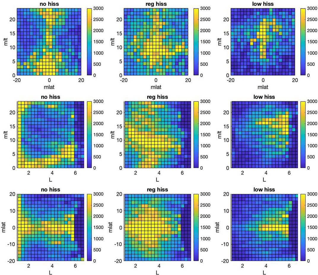
FIGURE 1. Distribution of spectral hiss classes: left column - “no hiss”; center column—“regular hiss”; right column - “low frequency hiss”; top row—(MLT, MLAT); middle row - (MLT, L); bottom row - (MLAT, L); color bar corresponds to class membership (number count of spectral shapes) in a given bin.

Figure 1 shows binned distribution of resulting plasmaspheric hiss spectral classes in different 2D planes of (MLAT, MLT, L) coordinates, where MLAT is magnetic latitude, MLT is magnetic local time, and L is spatial location (L-shell) in Earth radii. The spectral classes occupy distinct and different regions that are largely separated from each other, especially in the (MLT, L) plane. Figure 2 shows occurrence rate obtained by normalizing distribution in Figure 1 by normalizing to the total samples of all three spectral classes in each bin. Furthermore, different classes tend to occur in separate sectors of (MLAT, MLT, L) space, in agreement with Figures 1, 2 indicates that low-frequency hiss occurs more frequently from noon to dusk sector and at a larger L (≳ 5), which is generally similar to results of Shi et al. (2017). On the other hand, regular hiss is more dominant around noon sector. He et al. (2020, 2021) have also studied distribution of hiss, reporting a larger coverage in MLT. However, direct comparison with these studies is complicated due to details and differences in definitions of hiss wave measurements, including that our spectral classification does not consider the wave amplitude but only the shape of the wave spectra, as well as various geomagnetic activity levels (such as AE index).

FIGURE 2

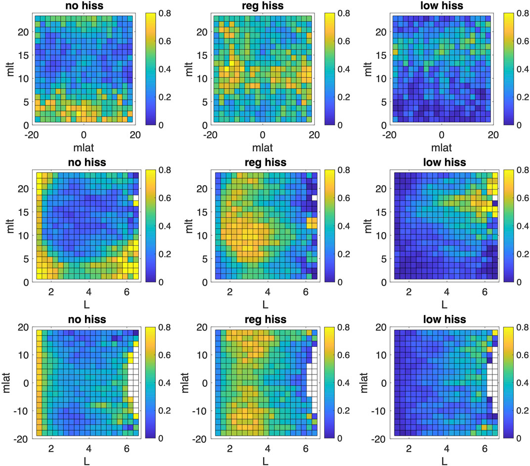
FIGURE 2. Same as in Figure 1 but normalized by the total number of spectral shapes for all three classes combined in each bin; white color corresponds to no data in the bin.

Random forests model

Random forests (RF) is an advanced classification procedure that generalizes classification and regression trees (CART); it is described in greater detail in Breiman (2001). The key idea is to assign a given data point to a class based on information contained in a set of predictors in an ensemble of regression or classification trees, or bag of trees. It is important to note that for RF the split into training and test dataset is done intrinsically during construction of the model. Each tree in the RF is constructed from a random sample of the training data, using sampling with replacement, and is then used to “predict” the class of each observation held out in the replacement when that tree was grown. The final classification of each observation is determined by a majority vote over all such tree-by-tree classifications. In our case, there are three classes of response variables, classified as “no hiss,” “regular hiss,” and “low-frequency hiss” event.

The most credible measures of RF model performance discussed in Sect. 3, such as classification errors, partial dependence scores, and receiver operating characteristics, are also derived from the held-out data. In addition, when each potential partitioning of the data is considered, only a random sample (without replacement) of predictors are candidates to define the split; this restriction helps one to take into account highly specialized predictors that fit only a few observations.

RF have several features that make the algorithm attractive for our purposes, among other machine learning methods. First, for the kinds of highly nonlinear and noisy relationships analyzed in this paper, there are no classifiers to date that consistently classify and forecast more accurately (Breiman, 2001). Second, it has been proven (Breiman, 2001) that RF does not overfit, which implies that the results will generalize well to new random samples from the same population. Third, because key performance measures are computed from the observations not used in tree construction, they are honest indicators of classification skill. Fourth, random forests provides informative plots of the relationships between inputs and outputs (i.e., predictors and predicted scores of spectral classes).

Results

For each data point, the RF classification model outputs a score in the [0, one] range for each of the three spectral classes, and the highest score determines the predicted class. Figure 3 shows the resulting overall classification error (fraction of misclassified observations) independent of the number of grown trees for RF models using different predictors. In addition to MLAT, MLT, and L-shell predictors, we have considered Kp, AE, and Dst geomagnetic indices, cold plasma density Ne, as well as solar wind V and solar wind dynamic pressure P. Recently, Malaspina et al. (2018) showed that plasmaspheric hiss waves power strongly depends on the plasmaspheric density and the location of the plasmapause. Hence, we additionally consider the location of plasmapause Lpp and distance from the plasmapause dL = L-Lpp as a RF predictor.

FIGURE 3

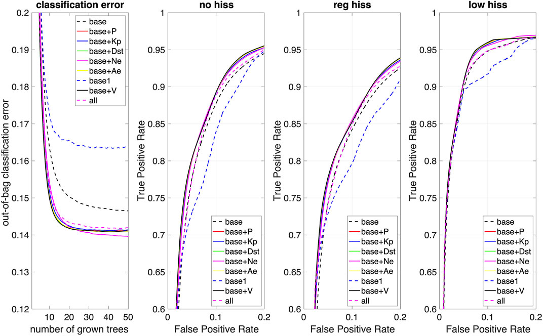
FIGURE 3. Overall classification error and receiver operating characteristic (ROC) curves (zoomed in) for predicting specific spectral classes of plasmaspheric hiss by random forest models using different predictors; “base” model—(MLAT, MLT, L); “base1” model — (MLAT, MLT, Lpp, dL) predictors; “all” model - all predictors.

The overall classification error of the “base” RF model using only MLAT, MLT, and L-shell predictors reaches the minimum and saturates at $\approx 0.15$, meaning that $\approx 85\%$ of data points are classified correctly. The classification error for given spectral class is also at $\approx 0.15$. On the other hand, the classification error of the “base1” model that utilizes information on the plasmapause location with (MLAT, MLT, Lpp, dL) predictors is a bit higher at 0.165. Adding to the “base” model, any other single predictor from the list of considered predictors, provides only a minor improvement in classification error to 0.14, and it is comparable to the one obtained when including all possible predictors in the “all” model.

A Receiver Operating Characteristic (ROC) curve informs on the quality of classifiers (such as RF) over a range of trade-offs between true positive and false positive error rates by applying threshold values across the interval [0,1] to classifier results. For a given threshold value and particular class i, true positive ratio (TPR) is the number of outputs whose actual and predicted class is class i, divided by the total number of outputs whose predicted class is class i, thus including also wrongfully made predictions. Similarly, false positive ratio (FPR) is the number of outputs whose actual class is not class i, but the predicted class is class i, divided by the number of outputs whose predicted class is not class i. Obtained ROC’s are presented in Figure 3 separately for each of spectral classes and different RF models, as well zoomed into the area of high TPR and small FPR, which both vary in [0 one] range. The larger area under the curve (AUC) values indicates a better classifier performance, and the perfect classifier would have the maximum AUC equal to 1, that is TPR being equal to one when FPR is zero. Resulting AUCs are very high, such as with a “base” RF model: $\approx 0.95$ for “no hiss” class, $\approx 0.94$ for “regular hiss” class, and $\approx 0.97$ for “low-frequency hiss” class, confirming overall very good predictive skill of RF.

Discussion

To help with interpretation of our RF results and understand the origin of such high predictive skill for our base model with MLAT, MLT and L predictors, we use partial dependence which quantifies the relationship between the subset of selected predictor variables X^S and predicted responses (scores of classes) by averaging remaining predictors X^C. A predicted response (in our case it is the score of three classes in the [0, one] range) f(X) depends on all MLAT, MLT and L predictor variables:

$f\left(X\right)=f\left(X^S,X^C\right).(1)$

The highest score among three classes determines the predicted class by RF model. The partial dependence is then estimated as:

$f^S\left(X^S\right)=\sum _{i=1}^{N}f\left(X^S,X_i^C\right),(2)$

where N is the number of observations and $X_i=(X_i^S,X_i^C)$ is the ith data point. We compute partial dependence in 2-D planes of (MLT, MLAT, L) coordinates; for example, X^S=(MLT, MLAT) and X^C = L, etc. Furthermore, we compute partial dependence of scores for each class and separately on the three subsets of our full dataset associated with three spectral classes: “no hiss”, “low-frequency hiss,” and “regular hiss,” shown in Figures 4–6, respectively. As can be seen from the 2-D partial dependence plots, the highest scores for the subset of data associated with a given spectral class, largely match the spatial distribution of that class on Figure 1, as well as exceeding scores of the other two classes. This model feature is most pronounced in MLT-L and is common for all partial dependence plots in Figures 4– 6. For example, the maximum of “low frequency hiss” class occurrence is roughly at 4 < L < 6 and 10 < MLT < 24 (Figure 1), same as for the one for 2-D partial dependence computed on the subset of ‘low frequency hiss” class (Figure 5). Similarly, the maximums of “no hiss” class occurrence and associated partial dependence are at narrow regions L < 1 or MLT < 10 (Figure 1 and Figure 4), while for the “regular hiss” these maximums are at 2 < L < 5 and 7 < MLT < 15. In other words, the RF model picks up the distinct spatial location of a given spectral class and yields the highest score with respect to other classes in that location. This feature explains a high predictive skill of RF model by using only these location-based predictors.

FIGURE 4

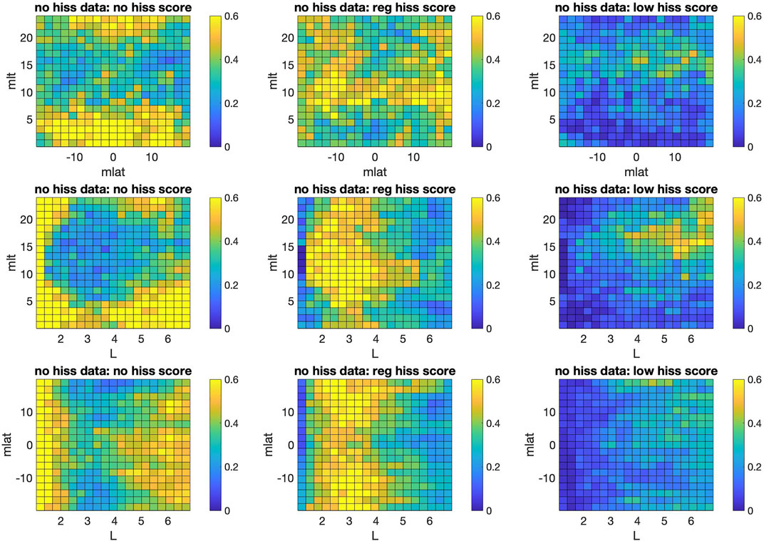
FIGURE 4. Partial dependence (Eq. 2) computed on the“no hiss” data points; color bar corresponds to the score of RF model.

FIGURE 5

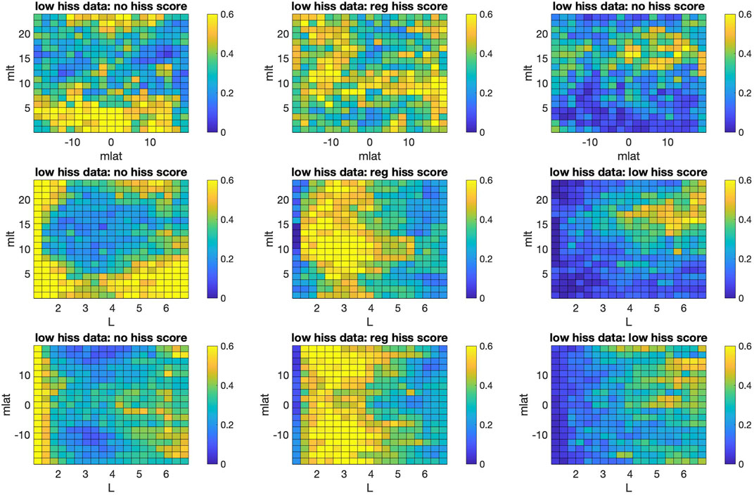
FIGURE 5. Partial dependence (Eq. 2) computed on “low-frequency hiss” data points; color bar corresponds to the score of RF model.

FIGURE 6

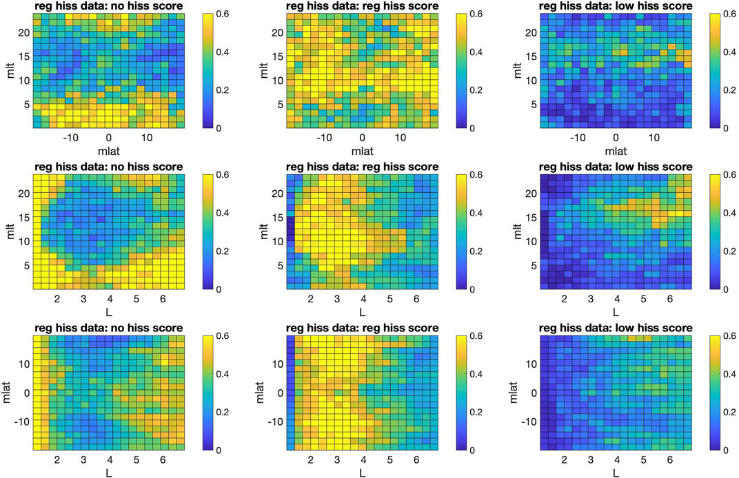
FIGURE 6. Partial dependence (Eq. 2) computed on “regular hiss” data points; color bar corresponds to the score of RF model.

Conclusion

We have developed the RF model for prediction of plasmaspheric hiss spectral classes obtained by SOM classification of the Van Allen Probes dataset. The RF model provides accurate prediction that is largely determined by distinct and different locations of a given spectral class in (MLAT, MLT, L) coordinate spaces, which are main predictors of the simplest RF base model. Adding any other single predictor among different magnetospheric, geomagnetic, and solar wind conditions provides only minor and similar incremental improvement in predictive skill, which is comparable to the one obtained when including all possible predictors.

A somewhat unexpected result is that adding predictors informing on the plasmapause location did not lead to a higher predictive skill. Because the SOM classification of plasmaspheric hiss spectral classes does not take into account the wave power, and considers spectral shape only, low-hiss class does not exclude the presence of regular hiss. If the classification model also were to take into account wave power, we might expect greater significance of plasmapause location, but this is beyond the scope of this study and is left for future research.

Data availability statement

The original contributions presented in the study are included in the article/supplementary material further inquiries can be directed to the corresponding author.

Author contributions

DK led the work, performed the RF analyses, and wrote the paper. AD advised on the interpretation and wrote the paper. DV developed SOM model. DM conceptualized the study and processed the observational data set that was used by DV in the SOM model.

Funding

This work was supported by NASA 80NSSC18K1034 award.

Acknowledgments

We thank Sharon Uy for proofreading this manuscript. We also thank two reviewers for helpful and constructive comments.

Conflict of interest

The authors declare that the research was conducted in the absence of any commercial or financial relationships that could be construed as a potential conflict of interest.

Publisher’s note

All claims expressed in this article are solely those of the authors and do not necessarily represent those of their affiliated organizations, or those of the publisher, the editors and the reviewers. Any product that may be evaluated in this article, or claim that may be made by its manufacturer, is not guaranteed or endorsed by the publisher.

References

Breiman, L. (2001). Random forests. Mach. Learn. 1, 5–32.

Google Scholar

Bristow, W. A., Topliff, C. A., and Cohen, M. B. (2022). Development of a high-latitude convection model by application of machine learning to SuperDARN observations. Space Weather 20, e2021SW002920. doi:10.1029/2021SW002920

CrossRef Full Text | Google Scholar

Engell, A. J., Falconer, D. A., Schuh, M., Loomis, J., and Bissett, D. (2017). Sprints: A framework for solar-driven event forecasting and research. Space Weather 15, 1321–1346. doi:10.1002/2017SW001660

CrossRef Full Text | Google Scholar

He, Z., Yu, J., Chen, L., Xia, Z., Wang, W., Li, K., et al. (2020). Statistical study on locally generated high-frequency plasmaspheric hiss and its effect on suprathermal electrons: Van allen probes observation and quasi-linear simulation. J. Geophys. Res. Space Phys. 125, e2020JA028526. doi:10.1029/2020JA028526

CrossRef Full Text | Google Scholar

He, Z., Yu, J., Li, K., Liu, N., Chen, Z., and Cui, J. (2021). A comparative study on the distributions of incoherent and coherent plasmaspheric hiss. Geophys. Res. Lett. 48, e2021GL092902. doi:10.1029/2021GL092902

CrossRef Full Text | Google Scholar

Kasapis, S., Zhao, L., Chen, Y., Wang, X., Bobra, M., and Gombosi, T. (2022). Interpretable machine learning to forecast SEP events for solar cycle 23. Space Weather 20, e2021SW002842. doi:10.1029/2021sw002842

CrossRef Full Text | Google Scholar

Kletzing, C. A., Kurth, W. S., Acuna, M., MacDowall, R. J., Torbert, R. B., Averkamp, T., et al. (2013). The electric and magnetic field instrument suite and integrated science (EMFISIS) on RBSP. Space Sci. Rev. 179, 127–181. doi:10.1007/s11214-013-9993-6

CrossRef Full Text | Google Scholar

Kondrashov, D., Shen, J., Berk, R., D’Andrea, F., and Ghil, M. (2007). Predicting weather regime transitions in Northern Hemisphere datasets. Clim. Dyn. 29, 535–551. doi:10.1007/s00382-007-0293-2

CrossRef Full Text | Google Scholar

Li, W., Ma, Q., Thorne, R. M., Bortnik, J., Kletzing, C. A., Kurth, W. S., et al. (2015). Statistical properties of plasmaspheric hiss derived from van allen probes data and their effects on radiation belt electron dynamics. JGR. Space Phys. 120, 3393–3405. doi:10.1002/2015JA021048

CrossRef Full Text | Google Scholar

Malaspina, D. M., Jaynes, A. N., Hospodarsky, G., Bortnik, J., Ergun, R. E., and Wygant, J. (2017). Statistical properties of low-frequency plasmaspheric hiss. JGR. Space Phys. 122, 8340–8352. doi:10.1002/2017JA024328

CrossRef Full Text | Google Scholar

Malaspina, D. M., Ripoll, J.-F., Chu, X., Hospodarsky, G., and Wygant, J. (2018). Variation in plasmaspheric hiss wave power with plasma density. Geophys. Res. Lett. 45, 9417–9426. doi:10.1029/2018GL078564

CrossRef Full Text | Google Scholar

Meredith, N. P., Horne, R. B., Kersten, T., Li, W., Bortnik, J., Sicard, A., et al. (2018). Global model of plasmaspheric hiss from multiple satellite observations. JGR. Space Phys. 123, 4526–4541. doi:10.1029/2018JA025226

CrossRef Full Text | Google Scholar

Millan, R. M., and Thorne, R. M. (2007). Review of radiation belt relativistic electron losses. J. Atmos. Sol. Terr. Phys. 69, 362–377. doi:10.1016/j.jastp.2006.06.019

CrossRef Full Text | Google Scholar

Reep, J. W., and Barnes, W. T. (2021). Forecasting the remaining duration of an ongoing solar flare. Space Weather 19, e2021SW002754. doi:10.1029/2021sw002754

CrossRef Full Text | Google Scholar

Ripoll, J.-F., Claudepierre, S. G., Ukhorskiy, A. Y., Colpitts, C., Li, X., Fennell, J. F., et al. (2020). Particle dynamics in the earth’s radiation belts: Review of current research and open questions. J. Geophys. Res. Space Phys. 125, 1. doi:10.1029/2019ja026735

CrossRef Full Text | Google Scholar

Saikin, A., Drozdov, A., Malaspina, D. M., and Zhu, H. (2022). Low frequency plasmaspheric hiss wave activity parametrized by plasmapause location: Models and simulations. ESSOAr. doi:10.1002/essoar.10511948.1

CrossRef Full Text | Google Scholar

Shi, R., Li, W., Ma, Q., Reeves, G. D., Kletzing, C. A., Kurth, W. S., et al. (2017). Systematic evaluation of low-frequency hiss and energetic electron injections. JGR. Space Phys. 122, 10, 263–310, 274. doi:10.1002/2017JA024571

CrossRef Full Text | Google Scholar

Smith, A. W., Rae, I. J., Forsyth, C., Oliveira, D. M., Freeman, M. P., and Jackson, D. R. (2020). Probabilistic forecasts of storm sudden commencements from interplanetary shocks using machine learning. Space Weather 18, e2020SW002603. doi:10.1029/2020SW002603

CrossRef Full Text | Google Scholar

Thorne, R. M., Smith, E. J., Burton, R. K., and Holzer, R. E. (1973). Plasmaspheric hiss. J. Geophys. Res. 78, 1581–1596. doi:10.1029/ja078i010p01581

CrossRef Full Text | Google Scholar

Vech, D., and Malaspina, D. M. (2021). A novel machine learning technique to identify and categorize plasma waves in spacecraft measurements. JGR. Space Phys. 126, e2021JA029567. doi:10.1029/2021JA029567

CrossRef Full Text | Google Scholar

Vech, D., Malaspina, D. M., Drozdov, A., and Saikin, A. (2022). Correlation between bandwidth and frequency of plasmaspheric hiss uncovered with unsupervised machine learning. arXiv. doi:10.48550/ARXIV.2207.10505

CrossRef Full Text | Google Scholar

Wygant, J. R., Bonnell, J. W., Goetz, K., Ergun, R. E., Mozer, F. S., Bale, S. D., et al. (2013). The electric field and waves instruments on the radiation belt storm probes mission. Space Sci. Rev. 179, 183–220. doi:10.1007/s11214-013-0013-7

CrossRef Full Text | Google Scholar

Zewdie, G. K., Valladares, C., Cohen, M. B., Lary, D. J., Ramani, D., and Tsidu, G. M. (2021). Data-driven forecasting of low-latitude ionospheric total electron content using the random forest and LSTM machine learning methods. Space Weather 19, e2020SW002639. doi:10.1029/2020SW002639

CrossRef Full Text | Google Scholar