 K.-J. Hwang1*
 J. M. Weygand2
 D. G. Sibeck3
 J. L. Burch1
 M. L. Goldstein4
 C. P. Escoubet5
 E. Choi1
 K. Dokgo1B. L. Giles3C. J. Pollock6D. J. Gershman3C. T. Russell2R. J. Strangeway2R. B. Torbert7
- 1Southwest Research Institute, San Antonio, TX, United States
- 2Institute of Geophysics and Planetary Physics, University of California, Los Angeles, Los Angeles, CA, United States
- 3NASA Goddard Space Flight Center, Greenbelt, MD, United States
- 4The Goddard Planetary Heliophysics Institute, University of Maryland, Baltimore County, MD, United States
- 5European Space Agency, Noordwijk, Netherlands
- 6Denali Scientific, LLC, Fairbanks, AK, United States
- 7Space Science Center, University of New Hampshire, Durham, NH, United States
The solar wind-magnetosphere interaction drives diverse physical processes on the flanks of Earth’s magnetopause, and in turn these processes couple to the ionosphere. We investigate simultaneous multipoint in-situ spacecraft and ground-based measurements to determine the role of Kelvin-Helmholtz waves at the Earth’s magnetopause and the low-latitude boundary layer in the magnetosphere-ionosphere coupling process. Nonlinear Kelvin-Helmholtz waves develop into flow vortices that twist and/or shear flux tube magnetic fields, thereby generating localized field-aligned currents. Kelvin-Helmholtz vortices on the dusk (dawn) flanks of the magnetosphere generate clockwise (counter-clockwise) rotations and upward (downward) field-aligned currents inside the flux tubes, consistent with the region-1 field-aligned current. We present in-situ MMS and Cluster spacecraft observations of Kelvin-Helmholtz vortices at the magnetopause that map to the poleward edge of the auroral regions. The FAST spacecraft and the ground-based magnetometers from which spherical elementary currents (acting as a proxy for vertical currents) can be calculated observe corresponding field-aligned current signatures. This study demonstrates the role played by the Kelvin-Helmholtz waves in linking magnetopause boundary fluctuations to ionospheric phenomena.
1 Introduction
In contrast to the Dungey (1961) model that refers to the transport of the solar wind into the Earth’s magnetosphere via dayside-then-nightside magnetic reconnection, (Axford and Hines, 1961) proposed that there was a quasi-viscous interaction between the solar wind and the magnetosphere, powered by flow velocity shear. The Kelvin-Helmholtz instability (KHI) grows in such a velocity shear layer. Along the Earth’s magnetopause, across which there is a significant velocity shear between the fast anti-sunward magnetosheath and the relatively stagnant magnetosphere, Kelvin-Helmholtz waves (KHWs) are generated. KHWs develop nonlinearly into large-scale rolled-up Kelvin-Helmholtz vortices (KHVs) when the shear flow energy is greater than the magnetic energy along the shear flow direction (Chandrasekhar, 1961; Hasegawa, 1975). This KHI-unstable condition is often satisfied when the interplanetary magnetic field (IMF) is oriented nearly perpendicular to the shear flow direction, i.e., either due northward or southward. However, the magnetopause KHWs/KHVs have been less frequently observed during periods of the southward IMF (Kavosi and Raeder, 2015). Hwang et al. (2011) and Nakamura et al. (2020) explained this: there exist decay mechanisms such as magnetic reconnection and flux transfer events that lead to a quick decay of the vortex structures under southward IMF.
KHWs/KHVs affect the Earth’s magnetosphere via various direct and indirect paths. Numerous studies have shown that nonlinear KHWs lead to mass, momentum, and energy transport across the magnetopause (Kivelson and Chen, 1995; Fairfield et al., 2000; Hasegawa et al., 2004; Faganello et al., 2008; Nakamura et al., 2013, 2017; Turkakin et al., 2013). In particular, large-scale KHVs promote solar wind entry into the magnetosphere via 1) magnetic reconnection between stretched magnetic field lines caused by the vortex motion (Otto and Fairfield, 2000; Nykyri and Otto, 2004; Cowee et al., 2010; Nakamura et al., 2011; Eriksson et al., 2016; Hwang et al., 2021) or mid-latitude reconnection between KHI-stable lobe fields and vortex-induced engulfed magnetosheath fields (Takagi et al., 2006; Faganello et al., 2012; Vernisse et al., 2016; Hwang et al., 2020; Eriksson et al., 2021), 2) diffusive transport through the turbulent decay of KHVs or coalescence of neighboring vortices (Matsumoto and Hoshino, 2004; Nakamura et al., 2004; Nakamura and Fujimoto, 2008; Cowee et al., 2009; Matsumoto and Seki, 2010), or 3) kinetic Alfvén waves or ion gyro-radius scale waves through a mode conversion from KH waves (Chaston et al., 2007; Yao et al., 2011). These processes result in plasma heating and the formation of a broad mixing layer along the flanks of the magnetosphere. Magnetohydrodynamic (MHD) simulations predict that flux tubes populated by plasmas of magnetosheath origin that enter the magnetosphere via KHVs can rapidly propagate toward the inner magnetosphere via an interchange instability (Wiltberger et al., 2000; Pembroke et al., 2012).
KHWs/KHVs can trigger ULF (ultra-low-frequency) pulsations in the Pc4-5 range with a frequency of ∼2–22 mHz via the excitation of a global cavity/waveguide mode that can occur at locations where the geomagnetic field-line eigenfrequency equals the frequency of KHWs (Mathie and Mann, 2000; Agapitov et al., 2009). KHW-driven ULF waves facilitate radial diffusion and/or acceleration of radiation belt electrons through drift resonance (Claudepierre et al., 2008). Nonlinear fast-mode waves can also develop at the edges of KHWs, propagate into the magnetosphere, and interact with radiation belt and ring current plasmas (Lai and Lyu, 2010).
The main focus of this paper is to study the influence of KHWs/KHVs on magnetosphere-ionosphere coupling (MIC). Previously, ionospheric traveling convection vortices have been interpreted as an ionospheric manifestation of solar wind dynamic pressure enhancements or KHI-driven ULF perturbations (Glassmeier and Heppner, 1992; Samson and Pao, 1996; Mann et al., 2002). Observations of ULF field-line-resonance pulsations initiated by magnetopause KHWs and conjugate ground-based magnetometer/radar measurements have shown the enhancements of electron precipitation or net downward Poynting flux and associated energy deposition into the ionosphere at latitudes coupled to the resonance region (Mann et al., 2002; Rae et al., 2007).
Those studies indicated that KHWs/KHVs have a global influence on the dynamics of the coupled magnetosphere-ionosphere system. In this paper, we incorporate the data obtained from Cluster, MMS, FAST, and ground magnetometers and show that KHWs/KHVs generate field-aligned currents (FACs) via the vortical motion that twists magnetic field lines within flux tubes. The sense of flux-tube rotation and associated FACs and conjugate ionospheric currents mapped to the dawn vs. dusk magnetopause KHWs/KHVs are very consistent with the region-1 FAC. This study demonstrates that KHWs/KHVs are at least partially responsible for the region1 FAC.
We organize this paper by introducing a theoretical prediction in Section 2, briefly describing the in-situ spacecraft and ground-based data used for this study in Section 3, presenting case studies of the dusk/dawn magnetopause KHW/KHV events observed by Cluster and MMS in Section 4 and Section 5, respectively. Discussion of Cluster/MMS case studies and conjugate ionospheric signatures and the implied roles and impact of KHWs/KHVs on MIC follow in Section 6.
2 Theoretical Expectation
Nonlinear KHWs drive flow vortices that cause a twist or shear of magnetic field lines within the vortical flux tube. This process generates FACs within the flux tube (see Figure 19 of Birn et al., 2004) as predicted by Maxwell’s equations:
B and E are the magnetic and electric field, respectively. J is the electric current density, and
V represents the plasma velocity. In case of small perturbations, the first-order terms of Eq. 2 for the component parallel to B yield (Paschmann et al., 2002)
The parenthesis in the right-hand side term is defined as flow vorticity,
Eq. 3 tells us that the gradient of vorticity gives rise to the generation of FACs. The magnitude of
3 Method
To test the theoretical prediction extracted from Eq. 3 observationally and to quantify how effectively and importantly KHV-driven FACs contribute to the region-1 current system, we use data from: the four Cluster spacecraft with the separation among the spacecraft greater than or equal to the ion gyroradius (
Both Cluster and MMS regularly fly through the dawn/dusk magnetopause and detect KHWs/KHVs. Their tetrahedral configuration facilitates the calculation of J using the curlometer technique (Dunlop et al., 2002). MMS further enables the direct estimation of
FAST traversed the northern and southern ionosphere with an altitude ranging from hundreds km to ≲4,000 km. Its operation during ∼12 years until 4 May 2009 enables conjunctions to be studied with KHWs/KHVs detected by Cluster. KHV events observed both by Cluster and most-recently-launched MMS can be coupled to ionospheric signatures recorded in ground magnetometers. Data obtained from 11 different magnetometer arrays (gMAG) allow us to calculate the (horizontal) equivalent ionospheric current (EIC) and the (vertical) spherical elementary current (SEC), which is a proxy for the field-aligned current, using the SEC technique outlined in Amm and Viljanen (1999) and Weygand et al. (2011).
From our coordinated case studies of in-situ magnetopause KHVs observed by Cluster and MMS and corresponding ionospheric responses identified by FAST or gMAG, we qualitatively test Eq. 3 in the dusk sector (Section 4) vs. the dawn sector (Section 5).
4 Duskward KHVs and Ionospheric FACs
4.1 Cluster Observations of Duskward KHVs
From 1,200 to 1300 UT on 20 November 2001 (Figures 1A–C) Cluster was located in the duskward magnetopause boundary layer. The four Cluster spacecraft (C1-4) were in a tetrahedral configuration and were separated by ∼1968 km on average (Figure 1D) with its barycenter at ∼[−5.3, 17.9, 3.2] Earth radii (RE) in Geocentric Solar Ecliptic (GSE) coordinates. [GSE coordinates correspond to the boundary normal coordinates (LMN) obtained from Shue et al. (1997) model in this event.] The IMF was mostly northward during this period. Figure 1 shows (A) the magnetic field (B) averaged over the four spacecraft and (B, C) the electric current density (J) obtained using the curlometer technique (x, y, and z components in blue, green, and red in GSE) and decomposed into parallel (red) and perpendicular (blue) components with respect to B. Both B and J show quasi-periodic fluctuations with a period of ∼8–15 min that are most likely to be attributed to magnetopause KHWs.
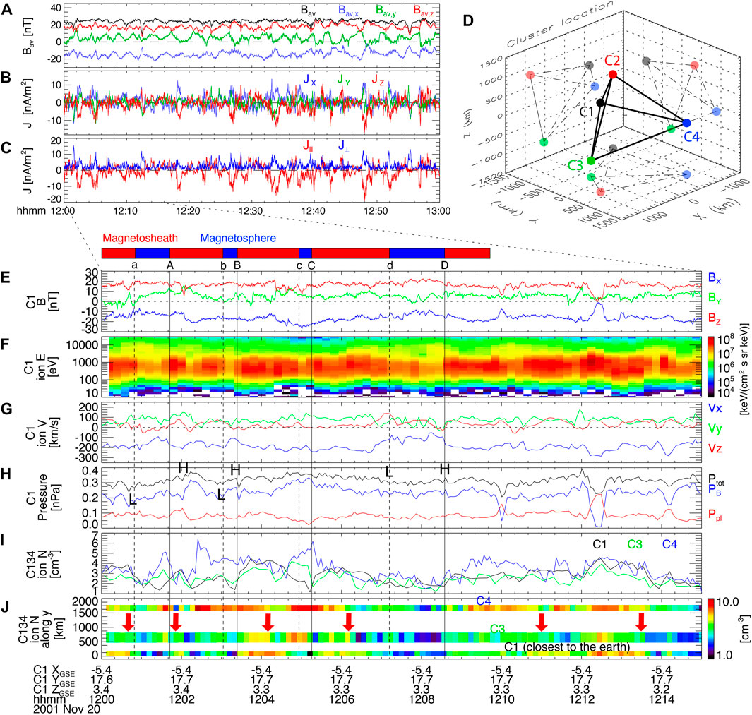
FIGURE 1. Cluster observation of duskward KHVs: (A) the magnetic field and (B,C) the electric current density during 1,200–1300 UT on 20 November 2001; (D) the tetrahedral configuration of the four Cluster spacecraft around its barycenter at ∼(−5.3, 17.9, 3.2) RE in GSE. C1 observation from 1200 UT to 1215 UT on 20 November 2001: (E) the magnetic field; (F) the ion energy spectrogram; (G) the ion velocity; (H) the plasma (red) and magnetic (blue) pressures, and the sum (black) of these pressures; (I) the ion density measured by C1 (black), C3 (green), and C4 (blue); (J) the ion density (color) at C1, C3, and C4 arranged in terms of their distance away from the magnetopause (along y; e.g., C1 located closest to the earth).
To test if these fluctuations resulted from nonlinear KHWs, we expanded the C1 data from 1200 UT to 1215 UT in Figures 1E–J. On the top of Figure 1E, we denoted a more-magnetospheric region in a blue bar as characterized by a relatively larger Bz (Figure 1E), more flux of high-energy (≳1 keV) ions (Figure 1F showing the ion energy spectrogram), reduced anti-sunward flow velocity (Vx shown in blue; Figure 1G) and ion density (black in Figure 1I). The region of a smaller Bz accompanied by more flux of low-energy ions (<1 keV), increases in anti-sunward velocity and ion density represents a more-magnetosheath side (red bar). [Note that the energy spectrogram indicates that the boundary layer was rather in a mixed/turbulent state.] We marked the magnetosphere-to-magnetosheath transitions by ‘A’, ‘B’, ‘C’, and ‘D’ at the top of Figure 1E and vertical solid black lines. The magnetosheath-to-magnetosphere transitions are marked by ‘a’, ‘b’, ‘c’, and ‘d’ and vertical dashed black lines.
In a steady state of KHVs, the centrifugal force is balanced by the pressure force. Since the centrifugal force is radially outward in a rolled-up vortex, the pressure force should point inward to the vortex center. The high total pressure, then, builds up at the boundary from the more-magnetospheric side into the more-magnetosheath side crossing by Cluster (see Figure 19 of Hasegawa, 2012). And the total pressure is minimized close to the boundary from the more-magnetosheath side to the more-magnetospheric side crossing. Figure 1H shows this trend. The total pressure (black), i.e., the sum of plasma (red) and magnetic (blue) pressures, often peaks at boundaries toward the more-magnetosheath side (‘H’ letters in Figure 1H) and decreases at boundaries toward the more-magnetospheric side (‘L’).
Another characteristic of KHVs is the so-called density reversal (Hasegawa et al., 2004). For the rolled-up vortices, the density profile away from the nominal magnetopause (i.e., ∼along + yGSE for duskward KHV events) shows a layer of a higher density (of magnetosheath origin) sandwiched between layers of a lower density (of magnetosphere origin). As a result, the spacecraft can detect a lower-density magnetosphere-origin layer located outward of a higher-density magnetosheath-origin layer. Figure 1I shows the ion density measured by C1 (black), C3 (green), and C4 (blue). Figure 1J presents these observations by color with C1, C3, and C4 data arranged in terms of their distance away from the magnetopause, i.e., along + yGSE. Red arrows in Figure 1J indicate the times when the density observed by C1 (closest to the earth) is higher than that observed by C3 or C4 (further away from the earth).
Both features of total pressure (Figure 1H) and density reversal (Figure 1J) support the identification of KHVs. For the duskward KHV event such as Figure 1, we expect the development of the antiparallel current or, equivalently, upward FAC in the northern ionosphere. Figure 1C, indeed, shows that J is donimantly antiparallel throughout the event.
4.2 FAST Observations of Ionospheric FACs
The geomagnetic field models (Tsyganenko, 1989; Tsyganenko, 1995) predict that the magnetic field lines encountered by Cluster during the Figure 1 event are mapped to the ionosphere at ∼73° LAT and ∼339° LON in geographic coordinates (GEO). FAST spacecraft fortuitously passed the northern ionosphere at/near the footprint of Cluster’s location around the time of the event. Figure 2 shows the energy spectrograms of down-going (with pitch angles of 0°
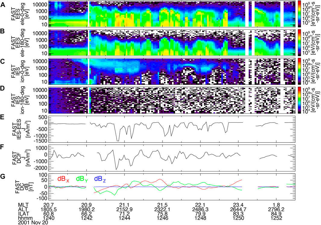
FIGURE 2. FAST observation of the northern ionosphere conjugate to the Cluster observation of duskward KHVs (Figure 1): the energy spectrograms of down-going [with pitch angles of 0°
4.3 MMS Observations of Duskward KHVs
During ∼1759–1809 UT on 1 October 2015, the MMS quartet with its barycenter at ∼[3.9, 9.2, −4.1] RE in Geocentric Solar Magnetospheric (GSM) coordinates encountered magnetopause fluctuations shown in Figure 3. The IMF was mostly southward during the period. A more-magnetosheath region is then identified by a mostly negative Bz (Figure 3A), more flux of <2 keV-energy ions (Figure 3B), larger anti-sunward flow (Figure 3C), enhanced ion density (Figure 3D), and reduced ion temperature (Figure 3E). We denoted such repeated regions by red bars on the top of Figure 3A (although the region between ‘E’ and ‘e’ at the top of Figure 1 is a mixed region exhibiting a magnetospheric field and a magnetosheath plasma). Opposite trends represent a more-magnetospheric region as indicated by a blue bar.
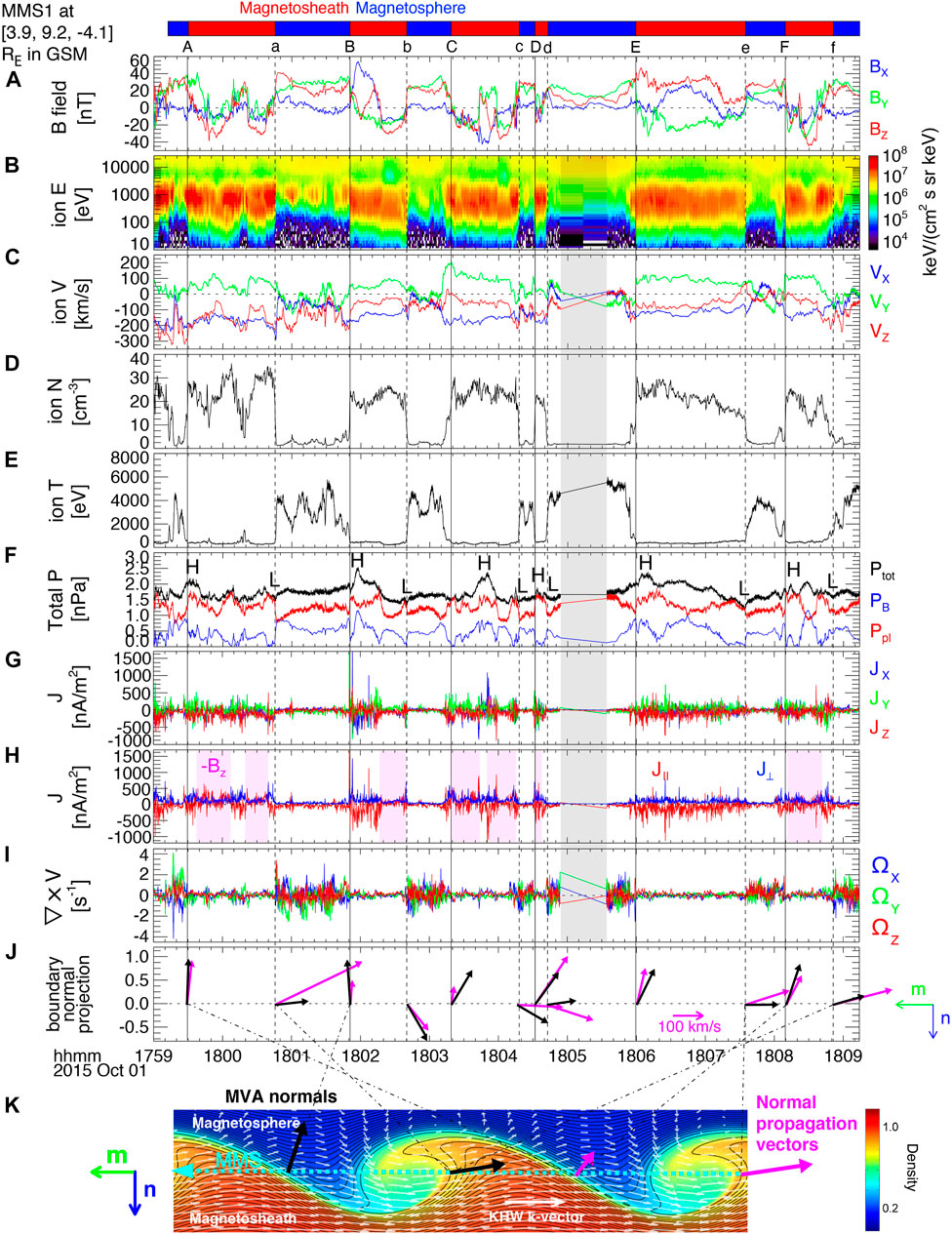
FIGURE 3. MMS1 observation of duskward KHVs during 1759–1809 UT on 1 October 2015: (A) the magnetic field; (B) the ion energy spectrogram; (C) the ion velocity; (D) the ion density; (E) the ion temperature; (F) the plasma (red) and magnetic (blue) pressures, and the sum (black) of these pressures; (G) the current density, J; (H) J decomposed into parallel (red) and perpendicular (blue) components; (I) the ion vorticity; (J) the mn-plane projections of boundary normals (black arrows) and normal propagation velocities (magenta arrows) to be compared with (K) typical waveforms of duskward KHVs, when viewed from north, with color representing density. The gray shade in (B–I) indicates a gap in the burst-mode particle data.
We, again, marked magnetosphere-to-magnetosheath transitions by ‘A’, ‘B’, …, ‘F’ at the top of Figure 3A with vertical solid black lines and magnetosheath-to-magnetosphere transitions by ‘a’, ‘b’, …, ‘f’ with vertical dashed black lines. Figure 3F shows that the total pressure generally rises at/near magnetosphere-to-magnetosheath boundaries (‘H’ in Figure 3F) and lowers at/near magnetosheath-to-magnetosphere boundaries (‘L’). This supports that the observed fluctuations are attributed to KHVs.
The average spacecraft separation of ∼31 km during this event prevents us from testing the density reversal. Instead, we performed boundary normal analyses. As shown in Figure 3K (Hwang et al., 2011, 2020), boundaries of typical KHVs tilt from the initially-undisturbed magnetopause with its normal along n, showing a more-gentle waveform at the trailing edges (see black arrows at ‘A’, ‘B’, …, ‘F’ in Figure 3K) and a steeper waveform at the leading edges (black arrows at ‘a’, ‘b’, …. ‘f’). Also, since KHVs propagate tailward along the magnetopause (along
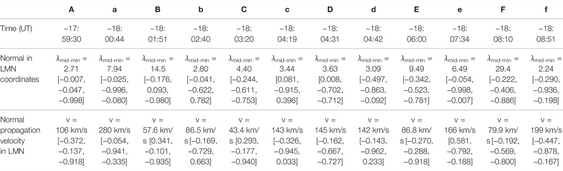
TABLE 1. Boundary normals and normal propagation vectors at the trailing (marked by vertical solid lines, A, B, …, F in Figure 3) and leading (vertical dashed lines, a, b, …, f) edges in LMN (λmid-min is the medium-to-minimum eigenvalue ratio in the minimum variance calculation.).
Figure 3J displays the mn-plane projections of boundary normals shown as black arrows and normal propagation velocities as magenta arrows. Both the normals and normal propagation vectors generally show a repetitive pattern between leading and trailing edges, consistent with Figure 3K. This confirms the identification of KHVs for the Figure 3 event.
Figure 3G shows J caculated from particle data (it is consistent with the curlometer-derived J) and Figure 3H shows parallel and perperdicular components of J. Both Jz and J||, although fluctuating around zero, are mostly negative with magenta shades in Figure 3H representing Bz < 0 periods. Therefore, J mainly pointed opposite to the geomagnetic B, consistent with the upward FAC in the northern ionosphere for the duskward KHV event.
Figure 3I shows the ion vorticity,
4.4 Ground Magnetometer Observations of Ionospheric FACs
The geomagnetic field model (Tsyganenko, 1989) predicts that the magnetic field lines encountered by MMS during the Figure 3 event are mapped to the ionosphere at ∼67° LAT and ∼302° LON. We use the gMAG data to derive the equivalent ionospheric current (EIC) and spherical elementary current (SEC). The result is shown in Figure 4, where the MMS footprint is denoted by a green dot. A counter-clockwise rotation of EIC around the green dot (upper panel) indicates upward FACs. SEC (lower), a proxy of the vertical current for an altitude of 100 km, shows the upward FAC of ∼18,400 A at the green dot. We note a bead-like structure in SEC indicative of upward FACs elongated in the east-west direction, possibly implying their generation via the duskward KHVs (Figure 3).
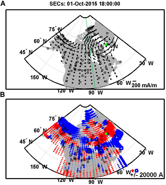
FIGURE 4. Ground magentometer observation of the ionospheric currents calculated from the SEC technique (Amm and Viljanen, 1999; Weygand et al., 2011) at 1800 UT on 1 October 2015: The (horizonal) equivalent ionospheric current [EIC; (A)] and the vertical spherical elementary current [SEC; (B)], which is a proxy of the FAC. The MMS footprint corresponding to the duskward KHV event (Figure 3) is denoted by a green dot.
5 Dawnward KHVs and Ionospheric FACs
5.1 Cluster Observations of Dawnward KHVs
From ∼0250 UT to ∼0430 UT on 28 July 2006 Cluster located at ∼[−13, −13, −3.0] RE in GSE observed KHV-induced magnetopause fluctuations (Figure 5) as reported by Hwang et al. (2011). [GSE coordinates that were close to GSM in this event correspond to the boundary normal coordinates (LMN) obtained from Shue et al. (1997) model.] The IMF was fluctuating with Bz
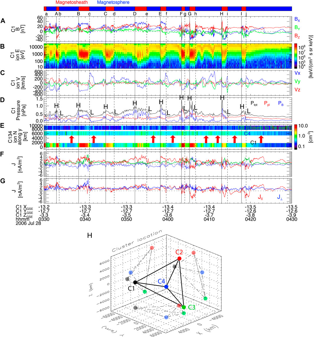
FIGURE 5. Cluster observation of dawnward KHVs during 0330–0430 UT on 28 July 2006: (A) the magnetic field and (B) the ion energy spectrogram; (C) the ion velocity; (D) the plasma (red), magnetic (blue), and total (black) pressures; (E) the ion density (color) measured by C1, C3, and C4 arranged in terms of their distance away from the magnetopause (along
The total pressure (black in Figure 5D) is maximized at/near the boundaries toward the more-magnetosheath region (‘H’) and minimized at boundaries toward the more-magnetospheric region (‘L’). The four Cluster spacecraft in a tetrahedron were separated by > 1 RE on average (Figure 5H), which enables us to test the density reversal. Figure 5E shows the ion density in color measured by C1/3/4 arranged in terms of their distance away from the magnetopause. Red arrows in Figure 5H mark the density-reversal times when the density observed by C4 or C3 (closer to the earth) is larger than that observed by C1 (further away from the earth). These observations confirm the dawnward-magnetopause KHVs for the Figure 5 event.
For the dawnward KHV event, we expect the development of the parallel current or, equivalently, downward FAC in the northern ionosphere (Section 2). Jz is, indeed, mostly positive (Figure 5F) and J|| is mainly parallel (Figure 5G) although the anti-paralell component becomes significant during later (near-) magnetosheath-side crossings (‘G’-‘h’, ‘H’-‘i’, around ‘j’). The overall trend is consistent with the prediction.
5.2 FAST Observations of Ionospheric FACs
The geomagnetic field models (Tsyganenko, 1989; Tsyganenko, 1995) predict that the footprint of the magnetic field lines encountered by Cluster at ∼0425 UT on 28 July 2006 falls at −69° LAT and ∼72° LON in GEO. FAST spacecraft fortuitously passed the conjugate southern ionosphere. Figure 6 shows the energy spectrograms of up-going (A, C) and down-going (B, D) electrons (A, B) and ions (C, D). During 0424:30-0426 UT precipitating fluxes of electrons are larger than up-going fluxes, and vice versa for ions. The difference between the ion and electron flux gives rise to the up-flowing FAC (Figure 6E) reaching −12,500 nA/m2 (dB data is not available). The up-flowing FAC in the southern ionosphere corresponds to the down-flowing FAC in the northern ionosphere, as expected for the dawnward KHVs of Figure 5.
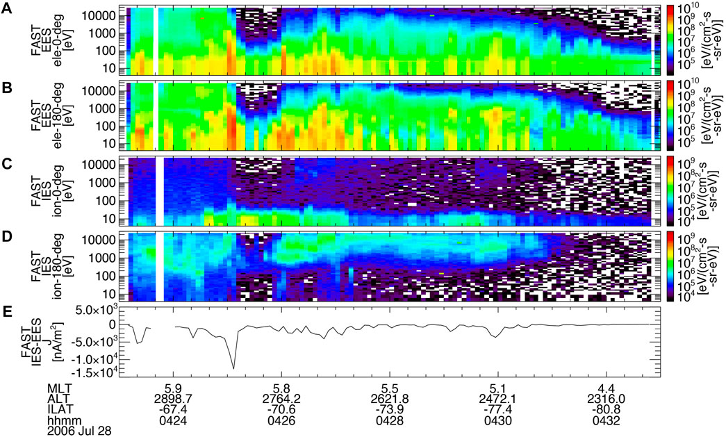
FIGURE 6. FAST observation of the southern ionosphere conjugate to the Cluster observation of dawnward KHVs (Figure 5): the energy spectrograms of down-going (with pitch angles of 0°
5.3 MMS Observations of Dawnward KHVs
During ∼1833–2015 UT on 6 February 2016, MMS observed the dawnward magnetopause/low-latitude boundary layer to be fluctuating. We focus on 7-min (1947–1954 UT) data when MMS with its average spacecraft separation of ∼17 km was located in the boundary layer at ∼[3.6, −9.3, −5.4]RE in GSM (Figure 7). The IMF was mostly duskward for the period. On the top of Figure 7A, blue (red) bars represent a more-magnetospheric (more-magnetosheath) region with more (less) flux of high-energy ions and electrons (Figures 7B,C), reduced (enhanced) anti-sunward flow and ion density (Figures 7D,E), and enhanced (reduced) ion temperature (Figure 7F). The magnetosphere-to-magnetosheath transitions are denoted by ‘A’, ‘B’, ‘C’, and ‘D’ with vertical solid black lines and the magnetosheath-to-magnetosphere transitions by ‘a’, ‘b’, ‘c’, and ‘d’ with vertical dashed black lines.
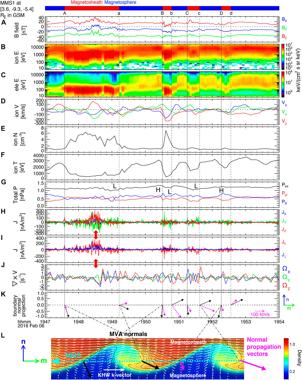
FIGURE 7. MMS1 observation of dawnward KHVs during 1947–1954 UT on 6 February 2016: (A) the magnetic field; (B) the ion energy spectrogram; (C) the electron energy spectrogram; (D) the ion velocity; (E) the ion density; (F) the ion temperature; (G) the plasma (red), magnetic (blue), and total (black) pressures; (H) the current density, J; (I) J decomposed into parallel (red) and perpendicular (blue) components; (J) the ion vorticity; (K) the mn-plane projections of boundary normals (black arrows) and normal propagation velocities (magenta arrows) to be compared with (L) typical waveforms of dawnward KHVs, when viewed from north, with color representing density.
The total pressure (black in Figure 7G) generally shows the typical ‘H’/‘L’ trend at magnetosphere-to-magnetosheath/magnetosheath-to-magnetosphere boundaries. To test the unique signature of leading vs. trailing edges of KHVs, we determined the nominal boundary normal coordinates (LMN) using Shue et al. (1997) model: l = [0.27, −0.26, 0.93], m = [−0.70, −0.72, 0.00], and n = [0.66, −0.65, −0.38] in GSM. Table 2 lists the normal propagation velocities derived using the four-spacecraft timing analysis and the MVA-derived boundary normals in LMN together with the medium-to-minimum eigenvalue ratio.
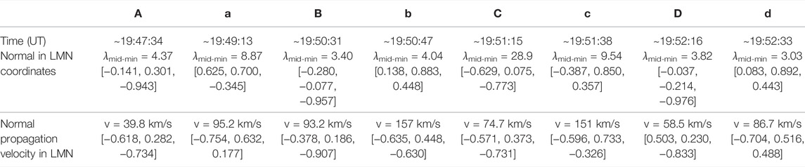
TABLE 2. Boundary normals and normal propagation vectors at the trailing (marked by vertical solid lines, A, B, C, and D in Figure 7) and leading (vertical dashed lines, a, b, c, and d) edges in LMN (λmid-min is the medium-to-minimum eigenvalue ratio in the minimum variance calculation.).
Figure 7K shows the mn-plane projection of boundary normals (black arrows) and normal propagation velocities (magenta arrows). Both the normals and normal propagation vectors are more aligned to
Figures 7H,I shows J caculated from the curlometer technique (decomposed into parallel and perperdicular components). Both Jz and J|| are mostly positive, in particular, during ‘A’-‘a’ (red arrows between Figures 7H,I). J mainly points due the geomagnetic B, consistent with the downward FAC in the northern ionosphere for the dawnward KHV event.
The ion vorticity,
5.4 Ground Magnetometer Observations of Ionospheric FACs
Figure 8 shows the EIC (upper) and SEC (lower) at 1951 UT (corresponding to the Figure 7 event) using the data from gMAG. The footprint of the magnetic field lines encountered by MMS at 1804 UT, i.e., prior to the Figure 7 event is predicted to sit on the ionosphere at ∼70° LAT and ∼230° LON in GEO from the Tsyganenko (1989) model (mapping failed after 1804 UT on 6 February 2016). A green dot in Figure 8 denotes the MMS footprint at 1804 UT. A generally clockwise rotation of EIC around the green dot indicates downward FACs. SEC shows an azimuthally-extended band of downward FACs at/around the green dot. Considering ∼1.8 h interval between 1804 UT and 1951 UT, it is likely that the footprint of MMS at 1951 UT falls within the downward FAC band (a green arrow), where the magnitude of downward FACs ranges from—
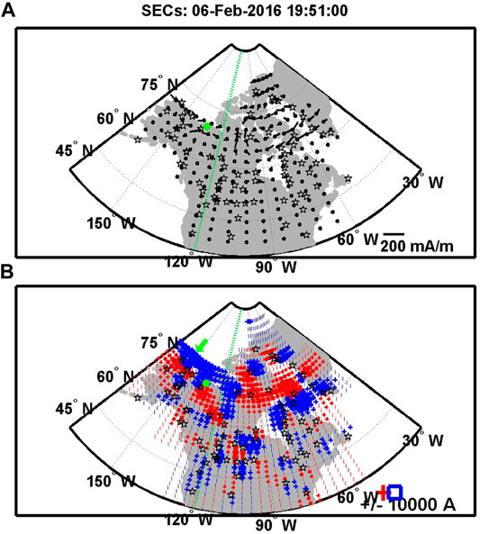
FIGURE 8. Ground magentometer observation of the ionospheric currents calculated from the SEC technique (Amm and Viljanen, 1999; Weygand et al., 2011) at 1951 UT on 6 February 2016: The (horizonal) equivalent ionospheric current [EIC; (A)] and the vertical spherical elementary current [SEC; (B)], which is a proxy of the FAC. The MMS footprint prior to (at 1804 UT) and during the dawnward KHV event (Figure 7) is denoted by a green dot and a green arrow (presumed), respectively.
6 Discussion
In this paper, we report coordinated Cluster/MMS observations of magnetopause KHVs and FAST/gMAG observations of ionospheric responses to those KHVs categorized into duskward vs. dawnward events. Cluster and MMS events presented in Section 4 and Section 5 demonstrate that nonlinear KHWs on the dusk (dawn) flank of the magnetosphere develop into flow vortices, which twist or shear flux tube magnetic fields in counter-clockwise (clockwise) rotation, generating upward (downward) FACs in the northern ionosphere. The sense of rotations is consistent with the region-1 Birkeland current system.
Table 3 lists our statistics of duskward (left columns) and dawnward (right) events including Figures 1–8 events. KHV-associated J|| or Jz ranges are obtained after low-pass filtering highly-fluctuating J data. ‘gMAG’-derived FAC ranges are obtained from the SEC data around the ionospheric footprint of MMS. For all MMS-gMAG conjunction events listed in Table 3, we identify the bead-like structure in SEC/FAC patterns elongated in the east-west direction (e.g., Figures 4, 8). This might support the generation of FACs via corresponding KHVs. We speculate that the characteristic time scale of the build-up of FACs into the ionosphere induced by low-latitude magnetopause KHVs is on the order of the Alfvén transit time (Johnson et al., 2021; Ebihara and Tanaka, 2022). This is hardly measurable in our study due to a limited knowledge on the developmental phase of KHVs that are locally observed by the spacecraft.
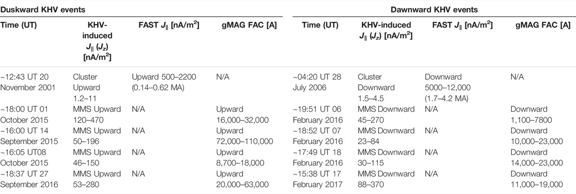
TABLE 3. List of coordinated Cluster/MMS observations of magnetopause KHVs and FAST/gMAG observations of ionospheric responses to those KHVs categorized into duskward (left columnes) vs. dawnward (right) events.
We note that the current density obtained from Cluster is less than that obtained from MMS by up to 2 orders of magnitude. This might be due to larger spacecraft separation of Cluster than MMS by ∼2 orders of magnitude. Since the size of a KHV (with a wavelength of ∼1.5–15 RE for the KHV events listed in Table 3; ∼3°–11° latitudinal or longitudinal width on ground) corresponds to the Cluster separation, we assume that the average current density induced by KHVs ranges from ∼1 to ∼10 nA/m2. The ratio between the current density associated with KHVs in the near-equatorial magnetopause (at Cluster) and in the ionosphere (at FAST) from Table 3 ranges from ∼200 to ∼4,000. This is relatively consistent with the ratio of magnetic flux-tube cross-section area between in-situ KHV locations and their conjugate ionosphere (∼1,000–6,000) based on the flux-tube current/magnetic-flux conservation.
Our statistics shown in Table 3 indicate that KHV-induced FACs categorized by duskward vs. dawnward KHVs correspond to FACs of region-1 sense. Considering the size of a KHV mapped to the ionosphere for the two Cluster events, the magnitude of FAC ranges 0.14–4.2 MA. This is comparable to the FAC magnitude obtained from gMAG for the MMS KHV events listed in Table 3. The order of region-1 current magnitudes often ranges 10−1 to 1 MA. Table 3, thus, indicates that KHVs might significantly contribute to region-1 current.
Previous studies attributed the generation of the region-1 current to magnetospheric pressure gradients (Yang et al., 1994; Iijima, 1997; Mishin et al., 2011) or speculated the region-1 current driver to be anti-sunward flows in the magnetosphere (Tanaka, 1998). Wing et al. (2011) investigated the variations of region-1 and 2 FACs as a function of solar wind and IMF. They showed that the response of FACs to solar wind velocity is higher for southward than for northward IMF, which is attributed to the higher velocity shear across the magnetopause boundary layer. A theory connecting the low-latitude shear flow or vortex and FACs in the ionosphere has been proposed (Johnson and Wing, 2015; Johnson et al., 2021). A theory-observation comparison was conducted by Johnson et al. (2021) and Petrinec et al. (2022). The theory is restricted to regions of upward region-1 FACs where a Knight current-voltage relation is generally valid.
So far as we know, our study presents the first observational evidence for the role played by KHVs in MIC, i.e., the generation of the global FAC system developed in both duskward and dawnward sectors: the magnetoapuse KHVs, at least partially and possibly significantly, contribute to the region-1 current system.
Data Availability Statement
The datasets presented in this study can be found in online repositories. The names of the repository/repositories and accession number(s) can be found in the article/Supplementary Material. The data from MMS, Cluster, FAST, and EIC/SEC data used for the present study are accessible through the public links http://lasp.colorado.edu/mms/sdc/public/, https://cdaweb.gsfc.nasa.gov/, and http://vmo.igpp.ucla.edu/data1/SECS/.
Author Contributions
K-JH found the research topic, analyzed the relevant data, and wrote the paper including tables and figures. JW provided/analyzed the EIC/SEC data. DS, JB, MG, EC, and KD assisted the data analysis and interpretation. CE, BG, CP, DG, CR, RS, and RT provided/assisted with the availability of the MMS data.
Funding
This study was supported, in part, by NASA’s MMS project at SwRI, NASA 80NSSC18K1534, 80NSSC18K0570, 80NSSC18K0693, and 80NSSC18K1337, and ISSI program: MMS and Cluster observations of magnetic reconnection.
Conflict of Interest
Author, Dr. C. J. P is employed by Denali Scientific, LLC, Fairbanks, AK.
The remaining authors declare that the research was conducted in the absence of any commercial or financial relationships that could be construed as a potential conflict of interest.
The reviewer PY declared a shared affiliation with the author(s) MG to the handling editor at the time of review.
Publisher’s Note
All claims expressed in this article are solely those of the authors and do not necessarily represent those of their affiliated organizations, or those of the publisher, the editors and the reviewers. Any product that may be evaluated in this article, or claim that may be made by its manufacturer, is not guaranteed or endorsed by the publisher.
References
Agapitov, O., Glassmeier, K.-H., Plaschke, F., Auster, H.-U., Constantinescu, D., Angelopoulos, V., et al. (2009). Surface Waves and Field Line Resonances: A THEMIS Case Study. J. Geophys. Res. 114, a–n. doi:10.1029/2008JA013553
Amm, O., and Viljanen, A. (1999). Ionospheric Disturbance Magnetic Field Continuation from the Ground to the Ionosphere Using Spherical Elementary Current Systems. Earth Planet Sp., 51, 431–440. doi:10.1186/bf03352247
Axford, W. I., and Hines, C. O. (1961). A Unifying Theory of High-Latitude Geophysical Phenomena and Geomagnetic Storms. Can. J. Phys., 39, 1433. doi:10.1139/p61-172
Birn, J., Raeder, J., Wang, Y. L., Wolf, R. A., and Hesse, M. (2004). On the Propagation of Bubbles in the Geomagnetic Tail. Ann. Geophys. 22, 1773–1786. doi:10.5194/angeo-22-1773-2004
Chandrasekhar, S. (1961). “Hydrodynamic and Hydromagnetic Stability,” in International Series of Monograph on Physics (Oxford: Clarendon), 652.
Chaston, C. C., Wilber, M., Mozer, F. S., Fujimoto, M., Goldstein, M. L., Acuna, M., et al. (2007). Mode Conversion and Anomalous Transport in Kelvin-Helmholtz Vortices and Kinetic Alfvén Waves at the Earth's Magnetopause. Phys. Rev. Lett. 99, 1750044. doi:10.1103/PhysRevLett.99.175004
Claudepierre, S. G., Elkington, S. R., and Wiltberger, M. (2008). Solar Wind Driving of Magnetospheric ULF Waves: Pulsations Driven by Velocity Shear at the Magnetopause. J. Geophys. Res. 113, a–n. doi:10.1029/2007JA012890
Cowee, M. M., Winske, D., and Gary, S. P. (2010). Hybrid Simulations of Plasma Transport by Kelvin-Helmholtz Instability at the Magnetopause: Density Variations and Magnetic Shear. J. Geophys. Res. 115, a–n. doi:10.1029/2009JA015011
Cowee, M. M., Winske, D., and Gary, S. P. (2009). Two-dimensional Hybrid Simulations of Superdiffusion at the Magnetopause Driven by Kelvin-Helmholtz Instability. J. Geophys. Res. Sp. Phys. 144, 14222. doi:10.14573/altex.2012.4.41110.1029/2009ja014222
Dungey, J. W. (1961). Interplanetary Magnetic Field and the Auroral Zones. Phys. Rev. Lett. 6, 47–48. doi:10.1103/PhysRevLett.6.47
Dunlop, M. W., Balogh, A., and Robert, P. (2002). Four-point Cluster Application of Magnetic Field Analysis Tools: The Curlometer. J. Geophys. Res. 107, 1–14. doi:10.1029/2001JA005088
Ebihara, Y., and Tanaka, T. (2022). Where Is Region 1 Field‐Aligned Current Generated? JGR Space Phys. 127, 1–15. doi:10.1029/2021ja029991
Eriksson, S., Ma, X., Burch, J. L., Otto, A., Elkington, S., and Delamere, P. A. (2021). MMS Observations of Double Mid-latitude Reconnection Ion Beams in the Early Non-linear Phase of the Kelvin-Helmholtz Instability. Front. Astron. Space Sci. 8, 1–24. doi:10.3389/fspas.2021.760885
Eriksson, S., Wilder, F. D., Ergun, R. E., Schwartz, S. J., Cassak, P. A., Burch, J. L., et al. (2016). Magnetospheric Multiscale Observations of the Electron Diffusion Region of Large Guide Field Magnetic Reconnection. Phys. Rev. Lett. 117, 15001. doi:10.1103/PhysRevLett.117.015001
Faganello, M., Califano, F., Pegoraro, F., and Andreussi, T. (2012). Double Mid-latitude Dynamical Reconnection at the Magnetopause: An Efficient Mechanism Allowing Solar Wind to Enter the Earth's Magnetosphere. Epl 100, 69001. doi:10.1209/0295-5075/100/69001
Faganello, M., Califano, F., and Pegoraro, F. (2008). Competing Mechanisms of Plasma Transport in Inhomogeneous Configurations with Velocity Shear: The Solar-Wind Interaction with Earth's Magnetosphere. Phys. Rev. Lett. 100, 1–4. doi:10.1103/PhysRevLett.100.015001
Fairfield, D. H., Otto, A., Mukai, T., Kokubun, S., Lepping, R. P., Steinberg, J. T., et al. (2000). Geotail Observations of the Kelvin-Helmholtz Instability at the Equatorial Magnetotail Boundary for Parallel Northward Fields. J. Geophys. Res. Space Phys., 105. 21159–2117310. doi:10.1029/1999ja000316
Glassmeier, K.-H., and Heppner, C. (1992). Traveling Magnetospheric Convection Twin Vortices: Another Case Study, Global Characteristics, and a Model. J. Geophys. Res. 97, 3977. doi:10.1029/91JA02464
Hasegawa, A. (1975). Plasma Instabilities and Non-linear Effects 430. New York, NY: Springer-Verlag.
Hasegawa, H., Fujimoto, M., Phan, T.-D., Rème, H., Balogh, A., Dunlop, M. W., et al. (2004). Transport of Solar Wind into Earth's Magnetosphere through Rolled-Up Kelvin-Helmholtz Vortices. Nature 430, 755–758. doi:10.1038/nature02799
Hasegawa, H. (2012). Structure and Dynamics of the Magnetopause and its Boundary Layers. Monogr. Environ. Earth Planets 1, 71–119. doi:10.5047/meep.2012.00102.0071
Hwang, K.-J., Dokgo, K., Choi, E., Burch, J. L., Sibeck, D. G., Giles, B. L., et al. (2021). Bifurcated Current Sheet Observed on the Boundary of Kelvin-Helmholtz Vortices. Front. Astron. Space Sci. 8, 1–13. doi:10.3389/fspas.2021.782924
Hwang, K.-J., Kuznetsova, M. M., Sahraoui, F., Goldstein, M. L., Lee, E., and Parks, G. K. (2011). Kelvin-Helmholtz Waves under Southward Interplanetary Magnetic Field. J. Geophys. Res. 116, a–n. doi:10.1029/2011JA016596
Hwang, K. J., Choi, E., Dokgo, K., Burch, J. L., Sibeck, D. G., Giles, B. L., et al. (2019). Electron Vorticity Indicative of the Electron Diffusion Region of Magnetic Reconnection. Geophys. Res. Lett. 46, 6287–6296. doi:10.1029/2019GL082710
Hwang, K. J., Dokgo, K., Choi, E., Burch, J. L., Sibeck, D. G., Giles, B. L., et al. (2020). Magnetic Reconnection inside a Flux Rope Induced by Kelvin‐Helmholtz Vortices. J. Geophys. Res. Space Phys. 125, 1–16. doi:10.1029/2019JA027665
Iijima, T., Potemra, T. A., and Zanetti, L. J. (1997). Contribution of Pressure Gradients to the Generation of Dawnside Region 1 and Region 2 Currents. J. Geophys. Res. 102, 27069–27081. doi:10.1029/97JA02462
Johnson, J. R., Wing, S., Delamere, P., Petrinec, S., and Kavosi, S. (2021). Field‐Aligned Currents in Auroral Vortices. J. Geophys. Res. Space Phys. 126, 1–15. doi:10.1029/2020JA028583
Johnson, J. R., and Wing, S. (2015). The Dependence of the Strength and Thickness of Field‐aligned Currents on Solar Wind and Ionospheric Parameters. J. Geophys. Res. Space Phys. 120, 3987–4008. doi:10.1002/2014JA020312
Kavosi, S., and Raeder, J. (2015). Ubiquity of Kelvin-Helmholtz Waves at Earth's Magnetopause. Nat. Commun. 6. doi:10.1038/ncomms8019
Kivelson, M. G., and Chen, S.-H. (1995). “The Magnetopause: Surface Waves and Instabilities and Their Possible Dynamical Consequences,” in Geophysical Monograph Series, 257–268. doi:10.1029/GM090p0257
Lai, S. H., and Lyu, L. H. (2010). A Simulation and Theoretical Study of Energy Transport in the Event of MHD Kelvin-Helmholtz Instability. J. Geophys. Res. 115, a–n. doi:10.1029/2010JA015317
Mann, I. R., Voronkov, I., Dunlop, M., Donovan, E., Yeoman, T. K., Milling, D. K., et al. (2002). Coordinated Ground-Based and Cluster Observations of Large Amplitude Global Magnetospheric Oscillations during a Fast Solar Wind Speed Interval. Ann. Geophys., 20, 405–426. doi:10.5194/angeo-20-405-2002
Mathie, R. A., and Mann, I. R. (2000). Observations of Pc5 Field Line Resonance Azimuthal Phase Speeds ’ A Diagnostic of Their Excitation Mechanism. J. Geophys. Res. Space Phys. 105. 10713–10728. doi:10.1029/1999ja000174
Matsumoto, Y., and Hoshino, M. (2004). Onset of Turbulence Induced by a Kelvin-Helmholtz Vortex. Geophys. Res. Lett. 31, 1–4. doi:10.1029/2003GL018195
Matsumoto, Y., and Seki, K. (2010). Formation of a Broad Plasma Turbulent Layer by Forward and Inverse Energy Cascades of the Kelvin-Helmholtz Instability. J. Geophys. Res. 115, a–n. doi:10.1029/2009JA014637
Mishin, V. M., Förster, M., Kurikalova, M. A., and Mishin, V. V. (2011). The Generator System of Field-Aligned Currents during the April 06, 2000, Superstorm. Adv. Space Res. 48, 1172–1183. doi:10.1016/j.asr.2011.05.029
Nakamura, T. K. M., Daughton, W., Karimabadi, H., and Eriksson, S. (2013). Three-dimensional Dynamics of Vortex-Induced Reconnection and Comparison with THEMIS Observations. J. Geophys. Res. Space Phys. 118, 5742–5757. doi:10.1002/jgra.50547
Nakamura, T. K. M., and Fujimoto, M. (2008). Magnetic Effects on the Coalescence of Kelvin-Helmholtz Vortices. Phys. Rev. Lett., 101, 1–4. doi:10.1103/PhysRevLett.101.165002
Nakamura, T. K. M., Hasegawa, H., Daughton, W., Eriksson, S., Li, W. Y., and Nakamura, R. (2017). Turbulent Mass Transfer Caused by Vortex Induced Reconnection in Collisionless Magnetospheric Plasmas. Nat. Commun. 8, 1–8. doi:10.1038/s41467-017-01579-0
Nakamura, T. K. M., Hasegawa, H., Shinohara, I., and Fujimoto, M. (2011). Evolution of an MHD-Scale Kelvin-Helmholtz Vortex Accompanied by Magnetic Reconnection: Two-Dimensional Particle Simulations. J. Geophys. Res. 116. doi:10.1029/2010JA016046
Nakamura, T. K. M., Hayashi, D., Fujimoto, M., and Shinohara, I. (2004). 92, 2–5. doi:10.1103/PhysRevLett.92.145001
Nakamura, T. K. M., Plaschke, F., Hasegawa, H., Liu, Y. H., Hwang, K. J., Blasl, K. A., et al. (2020). Decay of Kelvin‐Helmholtz Vortices at the Earth's Magnetopause under Pure Southward IMF Conditions. Geophys. Res. Lett. 47, 87574. doi:10.1029/2020GL087574
Nykyri, K., and Otto, A. (2004). Influence of the Hall Term on KH Instability and Reconnection inside KH Vortices. Ann. Geophys. 22, 935–949. doi:10.5194/angeo-22-935-2004
Otto, A., and Fairfield, D. H. (2000). Kelvin-Helmholtz Instability at the Magnetotail Boundary: MHD Simulation and Comparison with Geotail Observations. J. Geophys. Res. 105, 21175–21190. doi:10.1029/1999ja000312
Paschmann, G., and Daly, P. W. (1998). Analysis Methods for Multispacecraft Data. Bern: International Space Science Institute. Scientific Report 001.
Paschmann, G., Haaland, S., and Treumann, R. (2002). Chapter 3 - Theoretical Building Blocks. Space Sci. Rev. 103, 41–92. doi:10.1023/A:1023030716698
Pembroke, A., Toffoletto, F., Sazykin, S., Wiltberger, M., Lyon, J., Merkin, V., et al. (2012). Initial Results from a Dynamic Coupled Magnetosphere-Ionosphere-Ring Current Model. J. Geophys. Res. 117, a–n. doi:10.1029/2011JA016979
Petrinec, S. M., Wing, S., Johnson, J. R., and Zhang, Y. (2022). Multi-Spacecraft Observations of Fluctuations Occurring along the Dusk Flank Magnetopause, and Testing the Connection to an Observed Ionospheric Bead. Front. Astron. Space Sci. 9, 1–15. doi:10.3389/fspas.2022.827612
Rae, I. J., J Watt, C. E., Fenrich, F. R., Mann, I. R., Ozeke, L. G., and Kale, A. (2007). Energy Deposition in the Ionosphere through a Global Field Line Resonance. Available at: www.ann-geophys.net/25/2529/2007/.doi:10.5194/angeo-25-2529-2007
Samson, J. C., and Cogger, L. L, and Pao, Q. (1996). Observations of field line resonances, auroral arcs, and auroral vortex structures. J. Geophys. Res: Space Physics 101. 17373-17383. doi:10.1029/96ja01086
Shue, J.-H., Chao, J. K., Fu, H. C., Russell, C. T., Song, P., Khurana, K. K., et al. (1997). A New Functional Form to Study the Solar Wind Control of the Magnetopause Size and Shape. J. Geophys. Res. 102, 9497–9511. doi:10.1029/97JA00196
Siscoe, G. L., and Suey, R. W. (1972). Significance Criteria for Variance Matrix Applications. J. Geophys. Res.-Space 77, 1321–1322. doi:10.1029/JA077i007p01321
Sonnerup, B., and Scheible, M. (1998). Minimum and Maximum Variance Analysis. Anal. Methods Multi-Spacecr.185, 220. Available at: http://www.issibern.ch/forads/sr-001-08.pdf%0Ahttp://ankaa.unibe.ch/forads/sr-001-08.pdf.
Takagi, K., Hashimoto, C., Hasegawa, H., Fujimoto, M., and Tandokoro, R. (2006). Kelvin-Helmholtz Instability in a Magnetotail Flank-like Geometry: Three-Dimensional MHD Simulations. J. Geophys. Res. 111, 1–10. doi:10.1029/2006JA011631
Tanaka, T. (1998). “Generation Mechanism of the Field-Aligned Currrent System Deduced From a 3-D MHD Simulation of the Solar Wind-Magnetosphere-Ionosphere Coupling,” in Magnetospheric Research With Advanced Techniques, Editors R. L. Xu, and A. T. Y. Lui. (Pergamon, 1998a) Vol. 9, 133.
Tsyganenko, N. A. (1989). A Magnetospheric Magnetic Field Model With a Warped Tail Current Sheet. Planet. Space Sci. 37 (1), 5–20. doi:10.1016/0032-0633(89)90066-4
Tsyganenko, N. A. (1995). Modeling the Earth's Magnetospheric Magnetic Field Confined within a Realistic Magnetopause. J. Geophys. Res. 100, 5599. doi:10.1029/94ja03193
Turkakin, H., Rankin, R., and Mann, I. R. (2013). Primary and Secondary Compressible Kelvin-Helmholtz Surface Wave Instabilities on the Earth's Magnetopause. J. Geophys. Res. Space Phys. 118, 4161–4175. doi:10.1002/jgra.50394
Vernisse, Y., Lavraud, B., Eriksson, S., Gershman, D. J., Dorelli, J., Pollock, C., et al. (2016). Signatures of Complex Magnetic Topologies from Multiple Reconnection Sites Induced by Kelvin‐Helmholtz Instability. J. Geophys. Res. Space Phys. 121, 9926–9939. doi:10.1002/2016JA023051
Weygand, J. M., Amm, O., Viljanen, A., Angelopoulos, V., Murr, D., Engebretson, M. J., et al. (2011). Application and Validation of the Spherical Elementary Currents Systems Technique for Deriving Ionospheric Equivalent Currents with the North American and Greenland Ground Magnetometer Arrays. J. Geophys. Res. 116, 1–8. doi:10.1029/2010JA016177
Wiltberger, M., Pulkkinen, T. I., Lyon, G., and Goodrich, C. C. (2000). MHD Simulation of the Magnetotail during the December 10, 1996, Substorm. J. Geophys. Res. Space Phys. 105, 649–663. doi:10.1029/1999ja000251
Wing, S., Ohtani, S.-i., Johnson, J. R., Echim, M., Newell, P. T., Higuchi, T., et al. (2011). Solar Wind Driving of Dayside Field-Aligned Currents. J. Geophys. Res. 116, a–n. doi:10.1029/2011JA016579
Yang, Y. S., Spiro, R. W., and Wolf, R. A. (1994). Generation of Region 1 Currents by Magnetospheric Pressure Gradients. J. Geophys. Res. 99 (A1), 223–234. doi:10.1029/93JA02364
Keywords: Kelvin-Helmholtz vortices, Kelvin-Helmholtz waves, magnetosphere-Ionosphere coupling, region 1 field-aligned current, magnetopause and boundary layers, flow vorticity
Citation: Hwang K-J, Weygand JM, Sibeck DG, Burch JL, Goldstein ML, Escoubet CP, Choi E, Dokgo K, Giles BL, Pollock CJ, Gershman DJ, Russell CT, Strangeway RJ and Torbert RB (2022) Kelvin-Helmholtz Vortices as an Interplay of Magnetosphere-Ionosphere Coupling. Front. Astron. Space Sci. 9:895514. doi: 10.3389/fspas.2022.895514
Received: 13 March 2022; Accepted: 11 May 2022;
Published: 16 June 2022.
Edited by:
Toshi Nishimura, Boston University, United StatesReviewed by:
Xuanye Ma, Embry–Riddle Aeronautical University, United StatesPeter Haesung Yoon, University of Maryland, College Park, United States
Scott Alan Thaller, University of Colorado Boulder, United States
Copyright © 2022 Hwang, Weygand, Sibeck, Burch, Goldstein, Escoubet, Choi, Dokgo, Giles, Pollock, Gershman, Russell, Strangeway and Torbert. This is an open-access article distributed under the terms of the Creative Commons Attribution License (CC BY). The use, distribution or reproduction in other forums is permitted, provided the original author(s) and the copyright owner(s) are credited and that the original publication in this journal is cited, in accordance with accepted academic practice. No use, distribution or reproduction is permitted which does not comply with these terms.
*Correspondence: K.-J. Hwang, amh3YW5nQHN3cmkuZWR1