 E.-H. Kim
 J. R. Johnson
 K. Nykyri
95% of researchers rate our articles as excellent or good
Learn more about the work of our research integrity team to safeguard the quality of each article we publish.
Find out more
ORIGINAL RESEARCH article
Front. Astron. Space Sci. , 14 January 2022
Sec. Space Physics
Volume 8 - 2021 | https://doi.org/10.3389/fspas.2021.785413
This article is part of the Research Topic Micro- to Macro-Scale Dynamics of Earth’s Flank Magnetopause View all 17 articles
The Kelvin–Helmholtz (KH) instability of magnetohydrodynamic surface waves at the low latitude boundary layer is examined using both an eigenfrequency analysis and a time-dependent wave simulation. The analysis includes the effects of sheared flow and Alfvén velocity gradient. When the magnetosheath flows are perpendicular to the ambient magnetic field direction, unstable KH waves that propagate obliquely to the sheared flow direction occur at the sheared flow surface when the Alfvén Mach number is higher than an instability threshold. Including a shear transition layer between the magnetosphere and magnetosheath leads to secondary KH waves (driven by the sheared flow) that are coupled to the resonant surface Alfvén wave. There are remarkable differences between the primary and the secondary KH waves, including wave frequency, the growth rate, and the ratio between the transverse and compressional components. The secondary KH wave energy is concentrated near the shear Alfvén wave frequency at the magnetosheath with a lower frequency than the primary KH waves. Although the growth rate of the secondary KH waves is lower than the primary KH waves, the threshold condition is lower, so it is expected that these types of waves will dominate at a lower Mach number. Because the transverse component of the secondary KH waves is stronger than that of the primary KH waves, more efficient wave energy transfer from the boundary layer to the inner magnetosphere is also predicted.
The Kelvin–Helmholtz (KH) instability has been widely investigated in the Earth’s magnetosphere (Johnson et al., 2014). Unstable KH waves generally occur at the interface between two fluids having different velocities and are fundamentally important for understanding dynamics within the boundary layer that develops between the flows. These waves can affect the exchange of mass, momentum, and energy across those boundaries (e.g., Miura, 1984; Thomas and Winske, 1993; Otto and Fairfield, 2000; Nykyri and Otto, 2001; Matsumoto and Hoshino, 2006; Cowee et al., 2010; Hwang et al., 2011; Nakamura et al., 2011; Moore et al., 2016; Nykyri et al., 2017; Johnson et al., 2021). Mass transport due to KH instability can result from diffusion through thin boundaries created by the instability (e.g., Nakamura et al., 2017) and/or as the result of secondary reconnection (e.g., Otto and Nykyri, 2003; Ma et al., 2017) which results in more effective transport (Ma et al., 2019). Cross-scale energy transport associated with the KH instability may result from the generation of plasma waves leading to both ion and electron heating (Johnson and Cheng, 2001; Chaston et al., 2007; Moore et al., 2017; Nykyri et al., 2021a; Nykyri et al., 2021b; Delamere et al., 2021). The KH waves are also critical to the interaction between the solar wind and other planetary magnetospheres (McComas and Bagenal, 2008; Delamere and Bagenal, 2010; Delamere et al., 2021).
KH waves are surface waves because they are localized near the interface and exponentially decay away from the interface (e.g., Southwood, 1968; Pu and Kivelson, 1983). However, because the wave number is relatively small, the wave energy can still penetrate into the plasma sheet and/or the inner magnetosphere (e.g., Pu and Kivelson, 1983) and play a role in the generation of geomagnetic pulsations and mode conversion to the shear Alfvén waves (e.g., Chen and Hasegawa, 1974; Engebretson et al., 1998).
The magnetopause boundary is often assumed for simplicity to have zero thickness (Pu and Kivelson, 1983; Mills and Wright, 1999; Turkakin et al., 2013), and this assumption is valid for waves with wavelengths longer than the thickness of the boundary layer. When the shear velocity and the Alfvén speed jump at the zero-thickness interface, the linear dispersion relation of KH waves in a slab geometry for an incompressible plasma can be derived as follows (Chandrasekhar, 1961):
where ω and k are a wave frequency and vector, respectively, V and B are shear flow velocity and magnetic field, ρ and
is satisfied; and the stability threshold condition (2) may be used to determine a critical Alfvén Mach number (MAs) above which the KH wave is unstable.
In addition to the velocity transition at the magnetopause boundary, there is also a large gradient in the Alfvén velocity, which is typically wider in extent than the velocity shear layer (Paschmann et al., 1993). When an Alfvén velocity (VA) transition layer is included between the magnetosheath and magnetosphere, it can modify the KH wave properties. Strong coupling between the Alfvén surface wave and KH surface wave can result when the frequencies are comparable. This interaction between the two surface waves can lead to instability at a slower flow velocity. This new instability has been referred to as the resonant flow instability (RFI) as it results when Doppler-shifted compressional waves originating at the velocity interface have approximately the same frequency as the Alfvén resonance frequency (Taroyan and Erdélyi, 2003). The RFI includes a negative absorption of the magnetosonic waves, and it has been investigated for the solar corona (Tirry et al., 1998; Andries et al., 2000; Andries and Goossens, 2001; Taroyan and Ruderman, 2011; Antolin and Van Doorsselaere, 2019), magnetopause (Ruderman and Wright, 1998; Taroyan and Erdélyi, 2002, 2003), and magnetotail (Turkakin et al., 2014), respectively. While these works focused on shear in the velocity along the magnetic field direction, a similar instability can also result in velocity shear across the magnetic field or for discontinuous changes in the magnetic field direction at velocity interfaces. These modes can generally be referred to as secondary KH instabilities and are characterized by instability at a slower flow speed than the primary KH instability with growth occurring in a narrow range of propagation angle or Mach number (e.g., González and Gratton, 1994; Taroyan and Erdélyi, 2002; Turkakin et al., 2013). Turkakin et al. (2013) examined the primary and the secondary KH waves in the magnetopause and magnetotail when the magnetic fields in the magnetosheath and magnetosphere are perpendicular to each other. This mode may be particularly important during periods of low solar wind Alfvén Mach number (Lavraud and Borovsky, 2008; Lavraud et al., 2013; Génot and Lavraud, 2021) as it may be unstable even when the primary KH mode is stabilized. Although the (primary) KH wave is considered to be one source of the field-line resonances, the secondary KH instability is strongly coupled to the Alfvén waves. While it has been shown that the secondary KH instability is important in the solar corona, in this article, we show that the secondary KH waves also appear when the shear transition layer exists between the magnetosheath and magnetosphere. Using both eigenmode analysis and a newly developed time-dependent MHD wave model, detailed characteristics of the secondary waves are examined.
This article is structured as follows: in Section 2, the MHD wave equations are presented. Section 3 describes the dispersion relation of the KH waves when the zero-thickness interfaces are assumed. The eigenmode frequency, growth rate, and the KH wave amplitude ratio are also shown. In Section 4, we introduce a new time-dependent MHD wave simulation code. The simulation results are compared with the eigenfrequency analysis from Section 3. We also discuss the wave coupling between KH and Alfvén waves. The last section contains a brief discussion and conclusions.
In a cold plasma, basic equations of an ideal MHD plasma are
where ν is a collisional frequency that is introduced to damp waves propagating outside the region of interest, which effectively imposes outgoing boundary conditions. It should be noted that collisional effects play no role in the stability of the primary or secondary KH instabilities that we analyze in the rest of this article.
We assume that a field variable consists of background equilibrium (0) and small perturbation (1) components (B = B0 + B1, ρ = ρ0 + ρ1, and V = V0 + V1), and a shear flow
In Section 3, we solve the spectrum of eigenmodes of these equations in slab geometry, while in Section 4, we solve these equations using a finite-difference time-domain method.
To proceed with the spectral analysis, we define an auxiliary set of variables including the fluid displacement (ξ)
the total pressure perturbation (p), and compressibility (ψ),
Taking the Fourier transform in time
where
Then, Equations 11–17 can be reduced to two coupled first-order differential equations,
We solve Equations 18 and 19 to analyze the eigenmode frequency in Section 3.
Eigenfrequency analysis is performed when the shear transition layer exists between magnetosheath and magnetosphere. For calculations, V0 and VA are assumed to vary only in the direction of the x-axis, as shown in Figure 1A,
where Θ(x) = 0(x < 0) or 1(x ≥ 0) is a Heaviside step function. Figure 1A illustrates the transition from magnetosheath (I) to magnetosphere (III). The flow is sheared between regions I and II, while the Alfvén velocity increases between regions II and III. Region II is the shear layer, which divides the plasma into two semi-infinite homogeneous regions (I and III) separated with a width d. It is generally expected that velocity shear between layers I and II can drive a KH instability that is localized at this interface, while the jump in Alfvén velocity between regions II and III supports surface Alfvén waves satisfying the Alfvén resonance condition. In the following analysis, we show how these modes couple when the transitions occur in close proximity.
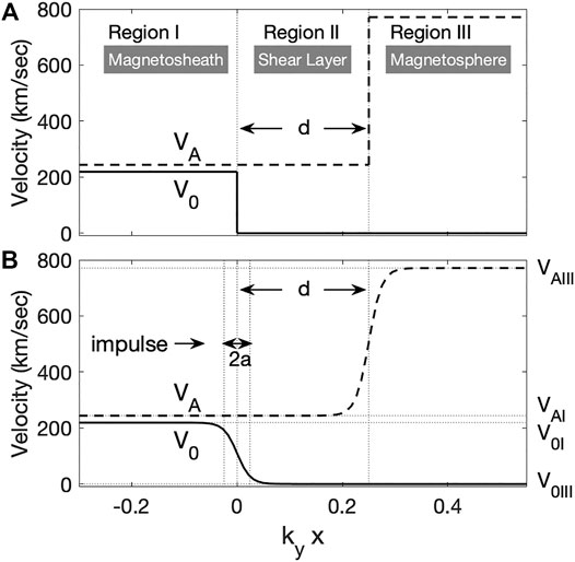
FIGURE 1. Illustration of the adopted background plasma profile. We assume (A) zero and (B) finite boundary width for eigenfrequency analysis and the numerical simulation, respectively. Regions I and III correspond to the magnetosheath and magnetosphere, respectively, and region II is the shear transition layer.
The eigenmodes of these equations are localized, so they must satisfy exponentially decaying boundary conditions in regions I and III. Moreover, it is also expected that in region II that the solution decays away from either boundary. As such, the analytical forms of the solutions in each region J are as follows:
where ± signs represent waves toward positive or negative directions in x.
For a surface wave, it is required that
and at x = d,
The wave dispersion relation is obtained by inserting the solutions into Equations 18 and 19 and noting that for solutions of the form exp(±κx) that
and the relationship between p and ξx in each region J = I, II, and III in Figure 1A becomes
where
From Equations 24–27 and 30, the wave dispersion can be derived as
The amplitude ratio (Ap) of the magnetic compressional component (p) between the two interfaces (x = 0 and d) can also be determined:
Using Equations 31 and 32, we calculate the eigenfrequency (ω), growth rate (γ), and amplitude ratio between magnetic compressional component (Ap) for various widths of the shear transition layer, kyd = 0, 0.25, 0.75, and 2.0, as shown in Figure 2. For these plots, the plasma densities in region I and region III are assumed to be N0I = 5 × 10⁶/m3 and N0III = 5 × 10⁵/m3, and the background magnetic field strength is B0 = 25nT. We also specify an angle of propagation (ϕ) with respect to the ambient magnetic field, ϕ = tan−1(ky/k‖) = 80° and
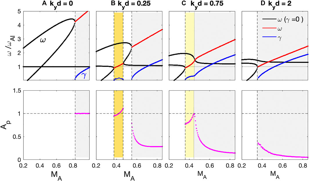
FIGURE 2. (Upper) Normalized eigenfrequencies (ω) and wave growth rate (γ) to Alfvén wave frequency at the magnetosheath (ωAI). (Lower) The amplitude ratio of the magnetic compressional component (Ap) at the two interfaces for kyd = 0, 0.25, 0.75, and 2.0, respectively.
In the absence of the shear transition layer (kyd = 0) as shown in Figure 2A, forward and backward propagating fast waves, which have positive and negative frequencies at MA = 0, occur when MA is small (Taroyan and Erdélyi, 2002). These waves are stable until MA reaches the threshold of the KH instability,
Introducing a finite width of the shear transition layer significantly changes the wave dispersion relations. In Figure 2, the PKHWs also occur for the cases of kyd ≠ 0. The MA threshold decreases from 0.83 for kyd = 0 to 0.35 for kyd = 2.0. Overall, the wave frequency ω decreases, while the growth rate γ increases as kyd increases. For example, for MA = 0.85, ω/ωAI = (4.35, 3.68, 2.95, 2.48) and γ/ωAI = (0.35, 1.5, 1.85, 1.89) when kyd = (0.0, 0.25, 0.75, 2.0). Thus, when a shear transition layer is included, lower frequency PKHWs are excited with a stronger growth rate and lower MA threshold.
For kyd = 0.25 in Figure 2B, coupling between the backward propagating fast and shear Alfvén waves occurs near ω/ωAI ∼ 1, and unstable waves also appear for 0.355 ≤ MA ≤ 0.47 (shaded yellow in Figure 2B). These waves correspond to the secondary KH waves (hereafter SKHW) (Turkakin et al., 2013). In this case, the SKHWs are clearly separated from the PKHWs and have lower ω, lower γ, and lower MA threshold than the PKHWs. The compressional amplitude ratio (Ap) in the lower panel shows significant differences between PKHWs and SKHWs; Ap ≪ 1 for the PKHWs and Ap ∼ 1 for the SKHWs. Therefore, for SKHWs, the amplitude of the instability is similar at both the V0 and VA interfaces, indicating a spreading of wave power over a more extended region, while the PKHWs are localized about the V0 interface. When the Mach number is low, it is expected that only the SKHWs would be excited.
When the VA interface is further away from the V0 interface (kyd = 0.75), as shown in Figure 2C, the PKHW and SKHW modes merge near MA ∼ 0.47. Although ω and γ monotonically increase as a function of MA, the KH waves have similar behavior to the SKHW (Ap ∼ 1 and ω ∼ ωAI) at smaller MA and the PKHWs (Ap < 1 and ω ≫ ωAI) at larger MA. Thus, the waves may still be divided into the semi-SKHW marked as a light yellow-shaded region and PKHW marked as a gray-shaded region in Figure 2C.
For kyd = 2, as shown in Figure 2D, only a single unstable wave mode corresponding to the PKHWs occurs localized at the V0 interface. The VA profile can be treated as a constant at the V0 interface and the MA threshold becomes MAs ∼ 2 tan−1(ϕ) = 0.359. The threshold occurs near ω/ωAI ∼ 1; thus, the wave frequencies are always higher than ωAI.
It is also useful to examine how ω and Ap depend on MA and kyd. Figure 3A,B shows contour plots of ω normalized to 1) ωKH0 and 2) ωAI, respectively. In this figure, two wave modes are clearly organized by ranges of MA; the PKHW for MA > 0.47 and the SKHW for 0.355 ≤ MA ≤ 0.47. Red and magenta lines in Figure 3A represent the MA threshold for the PKHW and SKHW, respectively. The MA threshold of the PKHWs decreases and the upper MA limit of the SKHWs increases as kyd increases. The thresholds merge near kyd ∼ 0.534 and MA ∼ 0.47. Thus, for MA > 0.47, a single wave mode appears (see Figure 2C); however, wave characteristics at lower and higher MA are significantly different.
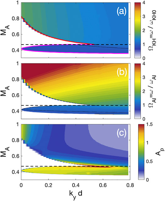
FIGURE 3. (A,B) Normalized eigenfrequencies to
The PKHWs show that all parameters (ω/ωKH0, ω/ωAI, and Ap) have a strong dependence on kyd, and they decrease as kyd increases. For most MA, ω/ωKH0 ∼ 1 and 1 < ω/ωKH0 < 2. Because both ω and ωKH0 increase proportionally to MA, ω/ωKH0 has less dependence on MA. However, because ωAI does not depend on ky and ω increases as MA increases, ω/ωAI depends on both MA and kyd. For the given conditions, ω/ωAI is maximized when kyd is small and MA is large. Figure 3C shows Ap < 1 for MA ≥ 0.47, except kyd → 0. Thus, it shows that the PKHWs are almost always dominant at the V0 interface. For kyd → 0, a strong amplitude of the pressure term occurs at the secondary interface. However, this increase in Ap is not an indicator of a separate instability, but rather it simply indicates that the decay of the wave power from the V0 interface to the VA interface reduced as the shear layer vanishes.
On the other hand, the eigenmode frequency of the SKHWs is comparable to ωKH0 and ωAI (0.9 ≤ ω/ωKH0(AI) ≤ 1.2) in the entire range of kyd and MA because this wave mode appears due to the coupling between shear Alfvén mode and the fast compressional waves (thus, ωKH0(AI) ∼ ωAI). For the entire range of kyd, Ap is always close to or even higher than 1. These results suggest that the KH instability occurs at both the V0 and VA interfaces with almost the same amplitude even though the interfaces are well separated.
The eigenmode calculations can be summarized as follows: the PKHWs are localized at the V0 interface having a higher frequency than ωA in the magnetosheath for faster shear flow velocity, while the SKHWs can be detected at both the V0 and VA interfaces with similar wave frequency to ωAI in the magnetosheath for slower shear flow velocity.
In order to examine the PKHWs and SKHWs, we also developed an MHD wave simulation model. Similar to the previous fluid wave simulation codes (Kim and Lee, 2003; Kim et al., 2007), the finite-difference method is used in both time and space to solve the MHD Equations 5–9 as an initial-valued problem. We adopt a box model in which B0 is assumed to lie along the z-direction and inhomogeneity is introduced in the x-direction, while the boundary layer plasma flows in the y-direction with variation in the x-direction. Perfect reflecting boundaries are assumed and strong collisions are applied near the boundaries to describe semi-infinite space. Therefore, the total energy of traveling waves decreases once the initial waves reach the boundary. Seed perturbations in the simulation domain result in linear growth of unstable modes, and the growth rate can be calculated once the unstable waves exceed the amplitudes of the initial perturbation.
We first examine the KH waves in a plasma where VA does not vary in space. In this simulation, a hyperbolic tangent V0 profile along with constant VA was adopted in the wave code:
where V0I is the flow velocity in region I, and this profile characterizes the V0 discontinuity in a scale length a, as shown in Figure 1B. One of the primary differences between the background profile used in the time-dependent analysis, and the previously discussed eigenmode analysis (a → 0) is the fact that the discontinuous profile has been smoothed.
We assume that the length of the simulation box is Lx ∼ 45/ky. Since the KH surface wave is expected to not fully decay by the time it reaches the edge of the simulation domain in the x-direction, we add an absorption layer near the boundary (∼30/ky) in the simulation box to prevent reflection. An initial perturbation is launched as a compressional component of V1x at the source location (kyxsource ∼ − 7.5) in region I (i.e., magnetosheath). This source is assumed to have a narrow spatial width (kyδsource = 0.093) and to include broadband frequencies,
Figure 4 shows the time evolution of the magnetic compressional component (B1z) in the x-direction for MA = 1 and kya = 0.025. Two vertical lines represent the source location (kya = − 7.5) and the V0 interface (kyx = 0), and thick dashed lines represent Alfvén speed (VA). Since the initial wave packet includes broadband frequencies, the wave packet disperses in time and space. Leftward propagating waves reach a strong collisional layer near the boundary (kyx < − 10.5) and are totally absorbed. Rightward propagating waves reach the V0 interface at kyx = 0 around t/tKH = 0.7, and they partially reflect from the interface due to a steepened density gradient. The rest of the waves penetrates the V0 interface and reach the collisional layer (kyx > 3.0). Once the magnetic field and velocities are perturbed near the interface, an unstable wave mode begins to grow at around t/tKH ∼ 1.2. Unlike the initial perturbation, these waves decay in the x-direction rather than propagate. The wave amplitude in Figure 4 saturates at ± 100.
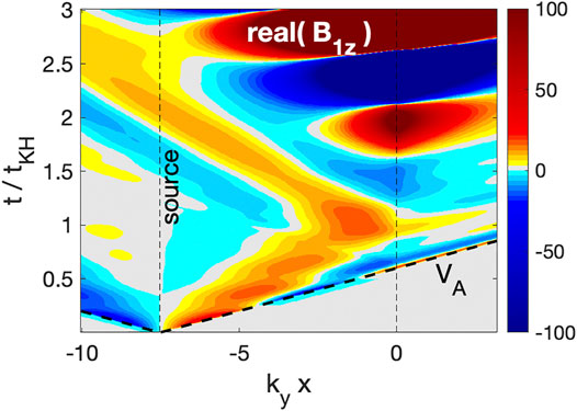
FIGURE 4. The time evolution of the magnetic compressional component (B1z) in the x-direction. The time and space are normalized to tKH = 2π/ωKH0 and ky, respectively. The interface is assumed to be located at kyx = 0. It is noted that the wave power is saturated at a 100 in this figure.
We focus on the surface waves at kyx = 0 and determine the growth rate, wave frequency, and polarization. Time histories of B1z and B1y at x = 0 in Figure 5A rapidly grow in time; thus, the sinusoidal wave form is not clearly seen. However, the wave growth term can be removed from the time histories using the magnetic (UB), kinetic energy (UV), or total energy (U = UB + UV). We plot Utot(t) = ∑xU(x, t) in the simulation box in Figure 6A. Early in the simulation period (t/tKH < 1.2) Utot is quasi-stable; however, once an unstable waves generated, it increases linearly. The wave magnetic field with a constant growth rate γ can be written as
and because of the magnetic energy UB ∝ |B|2, the wave growth rate γ in each grid point can be estimated from
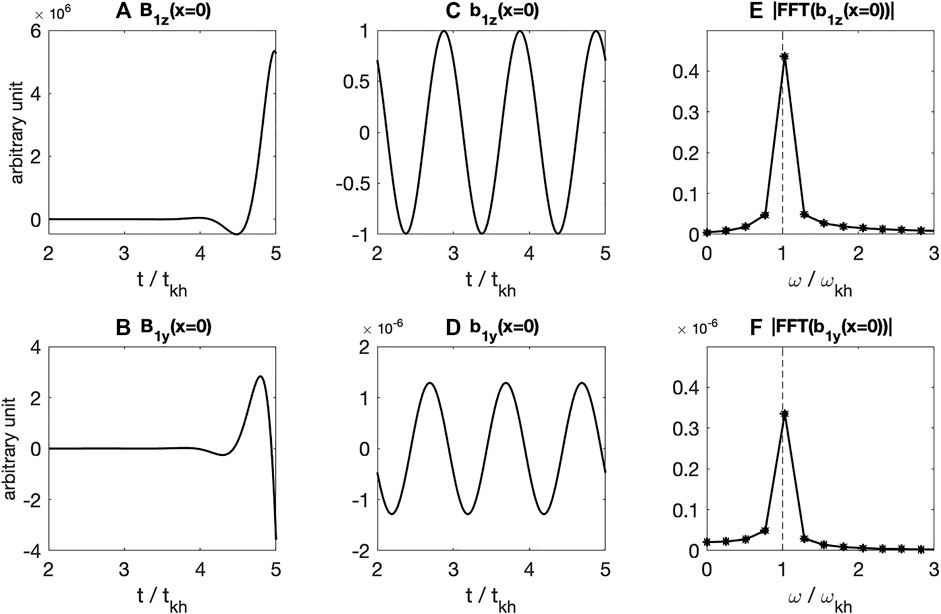
FIGURE 5. (A,B) Time histories of magnetic compressional (B1z) and transverse (B1y) components, (C,D) time histories removing the growth rate of b1z and b1y, and (E,F) fast Fourier transform in time of b1z and b1y at the interface (kyx = 0).
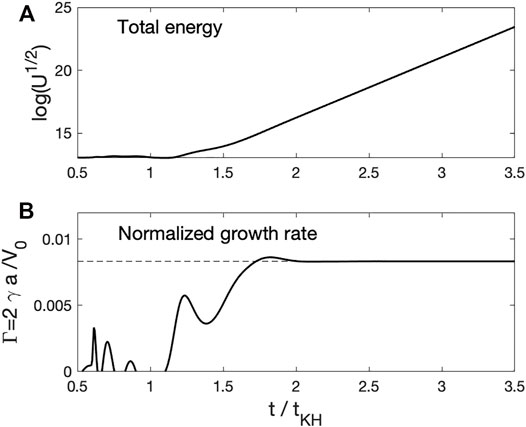
FIGURE 6. (A) Time evolution of wave energy (U) and (B) normalized growth rate (Γ = 2γa/V0I) in time.
We also confirmed that γ calculated using either the magnetic (UB) or kinetic energies (UV) are identical; thus,
When a boundary has a finite thickness, the normalized growth rate (Γ ≡ 2aγ/V0I) becomes a function of normalized boundary width (2kya) (Miura and Pritchett, 1982). To illustrate, the time evolution of Γ(t) is plotted in Figure 6B for kyd = 0.025 and MA = 1, and it converges to
Once the growth rate is determined, the wave components (and polarization) can be obtained from
where t0 is the time at which the wave growth begins. Figures 5C,D show that b1z and b1y have clear sinusoidal structures with a single frequency. The wave spectra of b1z and b1y in Figures 5E,F confirm that the single peak corresponds the KH wave frequency,
For code validation, we also compared the simulation results with prior analytical results in Miura and Pritchett (1982). Figure 7 shows the growth rate, Γ, as a function of (a) 2kya for MA = 1 and (b) as a function of MA for 2kya = 1. In this figure, the prior analytic results (gray lines) and our simulations (red stars) show excellent agreement with each other. For MA = 1 in Figure 7A, wave growth only occurs for a limited value of the normalized boundary width 0 < 2kya < 1.8 and maximizes near 2kya = 0.8. For 2kya = 1, the maximum Γ occurs for MA → 0 and has a value of 0.144, as predicted from Miura and Pritchett (1982). The growth rate decreases as MA increases and no KH wave arises for MA > 1.6. Therefore, the new MHD wave code successfully demonstrates KH waves and benchmarking comparisons of the simulations with previous analytical results validate the code accuracy.
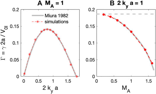
FIGURE 7. Normalized growth rates (Γ = 2γa/V0I) of KH surface waves (A) as a function of normalized tangential wavenumber 2kya for MA = 1 and (B) as a function of MA for 2kya = 1. Here, gray and red star dashed lines are from Miura and Pritchett (1982) and simulation results.
In this section, the simulation results include the shear transition layer between the magnetosphere and the magnetosheath, as shown in Figure 1B. In contrast to the results of Section 3, we consider a finite width of the boundary layer. Similar to the V0 profile in Equation 33, VA is assumed to have a hyperbolic tangent profile:
The two interfaces are separated with width d, although each interface has its own width, a. From the eigenfrequency calculations in Figure 2, we showed that the inclusion of a shear transition layer effectively generates the SKHWs when the shear flow velocity is slow; thus, we ran the simulations for kyd = 0.25 and 0.75 and MA < 0.85 to compare with the eigenmode calculation.
We used the time histories of b1, which does not include the exponential growth, in order to analyze the real frequency and relative strength of the field components. Figure 8 presents wave spectra of perturbed magnetic field and the Poynting flux for kyd = 0.25. For MA = 0.45 in Figure 8A, only the waves at ω/ωAI ∼ 1.2 have strong amplitude. This frequency is close to the eigenmode frequency of ω/ωAI = 1.17 in Figure 2. The estimated growth rate near the V0 and VA interfaces are identical with γ/ωAI = 0.128. This growth rate is also in good agreement with the analytical results of γ/ωAI = 0.142 in Section 3.
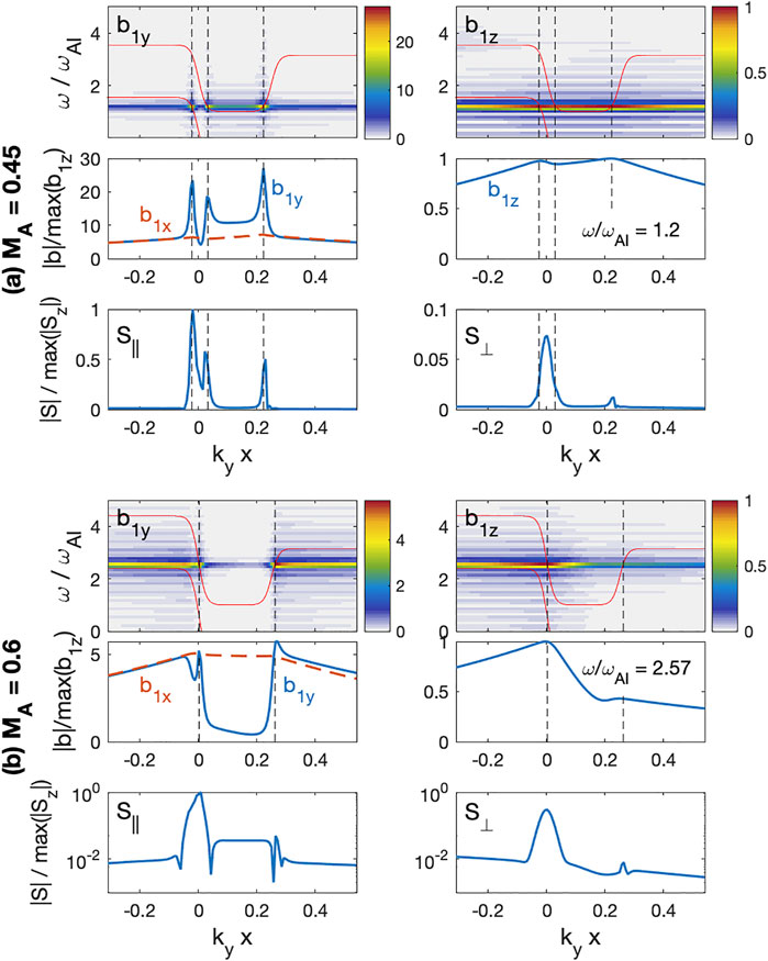
FIGURE 8. Wave spatial distribution for kyd = 0.25 (A) MA = 0.45 and (B) MA = 0.6. Upper panels are perturbed magnetic field compressional (b1z) and transverse (b1y) components, middle panels are the spatial structure of the peak frequency, and lower panels are the Poynting flux parallel (S‖) and perpendicular (S⊥) to B0.
In order to examine the detailed wave properties, we plot spatial structures of the fluctuating magnetic field (b1x, b1y, and b1z) at ω/ωAI = 1.2 in the middle row of Figure 8A. In this case, the compressional components (b1x and b1z) maximize at the VA and V0 interfaces and decay in the x-direction away from the interfaces. The b1z and b1x amplitudes at the two interfaces are comparable; thus, b1z(x = d)/b1z(x = 0) = 1.025. This ratio is almost identical to the amplitude ratio of the pressure Ap = 1.06 from Figure 2B.
On the other hand, the transverse component b1y is enhanced at three different locations near
Due to the finite width of the V0 interface near x = 0,
For the higher MA case in Figure 8B, the amplitude is maximized at ω = 2.57ωAI, which is similar to the analytical value of ω = 2.6ωAI in Section 3. The b1z component maximizes near x = 0 and the secondary peak near kyx = 0.25 becomes weaker. The b1z amplitude ratio between the two interfaces is 0.64, which is in good agreement with the analytical value of Ap = 0.4. The b1y component shows strong amplitude near kyx = 0 and kyx = 0.26. In this case, because the eigenmode frequency is higher than
For kyd = 0.75, the waves have a strong amplitude peak near ω/ωAI = 1.4 and 2.03 for MA = 0.45 and 0.6, respectively, and the spatial structures of these waves are presented in Figure 9. In this case, the PKHWs and SKHWs are not separated anymore (See Figure 2) and we define the KH waves in the lower MA as semi-SKHWs in Section 3. For MA = 0.45 in Figure 9A, b1z maximizes near x = 0 and a weak secondary peak appears near x = d. On the other hand, three amplitude peaks near kyx = − 0.025 4, 0.018, and 0.754 appear in b1y. The power ratio |b1y/max(b1z)| at the V0 interface is reduced to |b1y/max(b1z)| ∼ 7 from 23 for (kyd, MA) = (0.25, 0.45) in Figure 8A. The enhancement of S‖ is also seen at both interfaces and relatively strong S⊥ also appears. Near x = 0 at the V0 interface, |S⊥/S∥|x=0 is about 0.39, which is almost twice as large as |S⊥/S∥|x=0 = 0.195 for (kyd, MA) = (0.25, 0.45). Therefore, even though the compressional wave behavior of the semi-SKHWs is similar to the SKHWs, the mode conversion from semi-SKHWs becomes much weaker than that from the SKHWs.
For MA = 0.6 in Figure 9B, b1z decays along the x-direction from the V0 interface and no amplitude bump occurs at the VA interface. The b1y component shows a discontinuity at the VA interface following the compressional Alfvén wave dispersion relation. Therefore, S⊥ becomes comparable to S‖ for kyx > 0.75. In this case, the mode conversion at the VA interface does not occur, but energy still flows along the magnetic field line at the V0 interface.
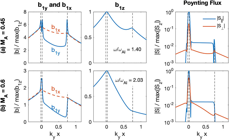
FIGURE 9. Wave spatial distribution for kyd = 0.75 (A) MA = 0.45 and (B) MA = 0.6.
We also analyzed the cases for MA for kyd = 0, 0.25, and 0.75 at various MA. Figure 10 shows the extracted eigenmode frequency and growth rate from the simulations. In this figure, the red and blue circled lines represent simulations, and the gray lines are taken from the eigenfrequency analysis from Figure 2 in Section 3. Although the boundary thicknesses used in Section 2 (slab) and Section 3 (width a) are different because the inhomogeneity scale length for the numerical simulation is much shorter than the wavelength, the eigenmode analytical and simulation results in ω and γ show excellent agreement.
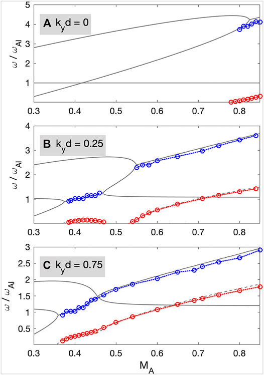
FIGURE 10. Calculated wave frequency (blue circles) and growth rate (red circles) from time-dependent simulations and eigenmode analysis (gray lines) for kyd = 0.25 and 0.75.
We also calculate the amplitude ratios between the compressional component at the two interfaces (Ap) and between transverse (b1y) and compressional
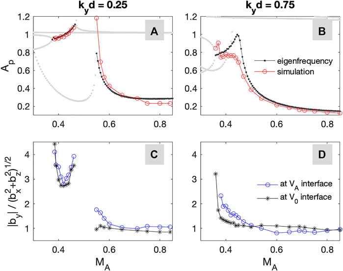
FIGURE 11. (A,B) Ap from the simulations (red circles) eigenfrequency calculations (black dots) for kyd = 0.25 and 0.75. (C,D) The amplitude ratio between the transverse and compressional components at the V0 interface (black stars) and the VA interface (blue circles), respectively.
This article investigates the coupling between KH and Alfvén waves when a shear transition layer exists between the magnetosheath and magnetosphere. Using the eigenfrequency analysis and time-dependent wave simulations, we showed that the SKHWs are generated when the shear velocity is slower than the typical threshold value for the onset of the KH instability.
The SKHWs occur with a frequency comparable to both KH wave frequency
The simulation results in Figures 8, 9 show that the magnetic transverse component is dominant at the interface and a strong field-aligned Poynting flux appears. Therefore, the energy transfer from the boundary layer to the Earth via mode-converted shear Alfvén waves occurs, which is similar to observations (Chaston et al., 2007). The wave simulations predict that a stronger mode conversion occurs from the SKHWs than from the PKHWs. However, the wave growth rate should be considered as well. Even though the mode conversion efficiency from the PKHWs is weaker than the SKHWs, the PKHWs amplitude can be strong enough due to the higher growth rate. Thus, a strong transverse component also can be detected from the PKHWs, but the compressional components are still comparable to the transverse components.
Although we clearly show the characteristics of PKHWs and SKHWs, this article only considers that the magnetic field is perpendicular to the flow velocity, and the magnetic field is assumed to be a constant. Indeed, the magnetic field in the magnetosheath and magnetosphere can be perpendicular in the magnetopause, and also the magnetic field and the flow velocity can be parallel in space, such as the solar corona and magnetotail. The secondary KH instability or resonant flow instability can occur under such conditions (Taroyan and Erdélyi, 2002, 2003; Turkakin et al., 2013). Furthermore, compressional waves bounded in the inner magnetosphere can contribute to the generation of the secondary KH instability (Turkakin et al., 2013) and also mode conversion to the shear Alfvén wave (Taroyan and Erdélyi, 2002). The total length of our numerical simulation model, including the collisional layer in Section 4, is somewhat comparable to
We also used a cold plasma approximation in the magnetosheath. The inclusion of thermal effects leads to an additional KH wave branch (Taroyan and Erdélyi, 2003). In warm plasmas, the Alfvén waves propagate as kinetic Alfvén waves (KAW). The KAW can have a larger wavenumber across the magnetic field line and field-aligned electric field and velocity components (Lin et al., 2010, 2012). Similar to Alfvén waves, KAW also transfers the energy away from the mode conversion location along the magnetic field line; thus, it is expected that a strong transverse component at each interface would also be detected with thermal effect.
In addition, a high level of turbulent fluctuations in the magnetosheath is observed in multiple satellites (e.g., Rakhmanova et al., 2021); however, nonlinear effects are not included in our analysis. It is possible that if these modes grow to sufficient amplitude, vortices will form and nonlinear interactions may become important, leading to plasma heating and transport. These nonlinear effects are left for future studies.
The raw data supporting the conclusions of this article will be made available by the authors, without undue reservation. Digital data can be found in the DataSpace of Princeton University http://arks.princeton.edu/ark:/88435/dsp013r074z09k
E-HK developed the real-time simulation code and ran both eigenfrequency calculation and simulation code, JRJ solved the dispersion relation of the KH waves and built the eigenfrequency calculation code, and KN discussed the observational background.
This material is based upon work supported by the United States Department of Energy, Office of Science, Office of Fusion Energy Sciences under contract DE-AC02-09CH11466. Work at Princeton University is under National Science Foundation (NSF) grant AGS1602855 and National Aeronautics and Space Administration (NASA) grants 80HQTR18T0066, 80HQTR19T0076, and NNX17AI50G. Work at Andrews University is supported by NASA grants NNX16AQ87G, 80NSSC19K0270, 80NSSC19K0843, 80NSSC18K0835, 80NSSC20K0355, NNX17AI50G, NNX17AI47G, 80HQTR18T0066, 80NSSC20K0704, and 80NSSC18K1578 and NSF grants AGS1832207 and AGS1602855. Work at Embry-Riddle Aeronautical University is under NASA grant NNX17AI50G.
The authors declare that the research was conducted in the absence of any commercial or financial relationships that could be construed as a potential conflict of interest.
All claims expressed in this article are solely those of the authors and do not necessarily represent those of their affiliated organizations, or those of the publisher, the editors, and the reviewers. Any product that may be evaluated in this article, or claim that may be made by its manufacturer, is not guaranteed or endorsed by the publisher.
Andries, J., and Goossens, M. (2001). Kelvin-Helmholtz Instabilities and Resonant Flow Instabilities for a Coronal Plume Model with Plasma Pressure. A&A 368, 1083–1094. doi:10.1051/0004-6361:20010050
Andries, J., Tirry, W. J., and Goossens, M. (2000). Modified Kelvin‐Helmholtz Instabilities and Resonant Flow Instabilities in a One‐dimensional Coronal Plume Model: Results for Plasma \documentclass{aastex} \usepackage{amsbsy} \usepackage{amsfonts} \usepackage{amssymb} \usepackage{bm} \usepackage{mathrsfs} \usepackage{pifont} \usepackage{stmaryrd} \usepackage{textcomp} \usepackage{portland,xspace} \usepackage{amsmath,amsxtra} \usepackage[OT2,OT1]{fontenc} \newcommand\cyr{ \renewcommand\rmdefault{wncyr} \renewcommand\sfdefault{wncyss} \renewcommand\encodingdefault{OT2} \normalfont \selectfont} \DeclareTextFontCommand{\textcyr}{\cyr} \pagestyle{empty} \DeclareMathSizes{10}{9}{7}{6} \begin{document} \landscape $\beta =0$ \end{document}. ApJ 531, 561–570. doi:10.1086/308430
Antolin, P., and Van Doorsselaere, T. (2019). Influence of Resonant Absorption on the Generation of the Kelvin-Helmholtz Instability. Front. Phys. 7, 85. doi:10.3389/fphy.2019.00085
Chandrasekhar, S. (1961). Hydrodynamic and Hydromagnetic Stability. Oxford, U.K.: Oxford University Press.
Chaston, C. C., Wilber, M., Mozer, F. S., Fujimoto, M., Goldstein, M. L., Acuna, M., et al. (2007). Mode Conversion and Anomalous Transport in Kelvin-Helmholtz Vortices and Kinetic Alfvén Waves at the Earth's Magnetopause. Phys. Rev. Lett. 99, 175004. doi:10.1103/PhysRevLett.99.175004
Chen, L., and Hasegawa, A. (1974). Plasma Heating by Spatial Resonance of Alfvén Wave. Phys. Fluids 17, 1399–1403. doi:10.1063/1.1694904
Cowee, M. M., Winske, D., and Gary, S. P. (2010). Hybrid Simulations of Plasma Transport by Kelvin-Helmholtz Instability at the Magnetopause: Density Variations and Magnetic Shear. J. Geophys. Res. 115, A06214. doi:10.1029/2009JA015011
Delamere, P. A., and Bagenal, F. (2010). Solar Wind Interaction with Jupiter's Magnetosphere. J. Geophys. Res. 115, A10201. doi:10.1029/2010JA015347
Delamere, P. A., Ng, C. S., Damiano, P. A., Neupane, B. R., Johnson, J. R., Burkholder, B., et al. (2021). Kelvin-Helmholtz‐Related Turbulent Heating at Saturn's Magnetopause Boundary. J. Geophys. Res. Space Phys. 126, e2020JA028479. doi:10.1029/2020JA028479
Engebretson, M., Glassmeier, K.-H., Stellmacher, M., Hughes, W. J., and Lühr, H. (1998). The Dependence of High-Latitude Pcs Wave Power on Solar Wind Velocity and on the Phase of High-Speed Solar Wind Streams. J. Geophys. Res. 103, 26271–26283. doi:10.1029/97JA03143
Génot, V., and Lavraud, B. (2021). Solar Wind Plasma Properties during Ortho-parker Imf Conditions and Associated Magnetosheath Mirror Instability Response. Front. Astron. Space Sci. 8, 153. doi:10.3389/fspas.2021.710851
González, A. G., and Gratton, J. (1994). The Role of a Density Jump in the Kelvin-Helmholtz Instability of Compressible Plasma. J. Plasma Phys. 52, 223–244. doi:10.1017/S0022377800017888
Hwang, K.-J., Kuznetsova, M. M., Sahraoui, F., Goldstein, M. L., Lee, E., and Parks, G. K. (2011). Kelvin-Helmholtz Waves under Southward Interplanetary Magnetic Field. J. Geophys. Res. 116, A08210. doi:10.1029/2011JA016596
Johnson, J. R., and Cheng, C. Z. (2001). Stochastic Ion Heating at the Magnetopause Due to Kinetic Alfvén Waves. Geophys. Res. Lett. 28, 4421–4424. doi:10.1029/2001gl013509
Johnson, J. R., Wing, S., and Delamere, P. A. (2014). Kelvin Helmholtz Instability in Planetary Magnetospheres. Space Sci. Rev. 184, 1–31. doi:10.1007/s11214-014-0085-z
Johnson, J. R., Wing, S., Delamere, P., Petrinec, S., and Kavosi, S. (2021). Field‐Aligned Currents in Auroral Vortices. J. Geophys. Res. Space Phys. 126, e28583. doi:10.1029/2020JA028583
Kim, E.-H., Cairns, I. H., and Robinson, P. A. (2007). Extraordinary-Mode Radiation Produced by Linear-Mode Conversion of Langmuir Waves. Phys. Rev. Lett. 99, 015003. doi:10.1103/physrevlett.99.015003
Kim, E.-H., and Lee, D.-H. (2003). Resonant Absorption of Ulf Waves Near the Ion Cyclotron Frequency: A Simulation Study. Geophys. Res. Lett. 30, 2240. doi:10.1029/2003gl017918
Lavraud, B., and Borovsky, J. E. (2008). Altered Solar Wind-Magnetosphere Interaction at Low Mach Numbers: Coronal Mass Ejections. J. Geophys. Res. 113, A00B08. doi:10.1029/2008JA013192
Lavraud, B., Larroque, E., Budnik, E., Génot, V., Borovsky, J. E., Dunlop, M. W., et al. (2013). Asymmetry of Magnetosheath Flows and Magnetopause Shape during Low Alfvén Mach Number Solar Wind. J. Geophys. Res. Space Phys. 118, 1089–1100. doi:10.1002/jgra.50145
Lin, Y., Johnson, J. R., and Wang, X. (2012). Three-Dimensional Mode Conversion Associated with Kinetic Alfvén Waves. Phys. Rev. Lett. 109, 125003. doi:10.1103/PhysRevLett.109.125003
Lin, Y., Johnson, J. R., and Wang, X. Y. (2010). Hybrid Simulation of Mode Conversion at the Magnetopause. J. Geophys. Res. 115, A04208. doi:10.1029/2009JA014524
Ma, X., Delamere, P. A., Nykyri, K., Burkholder, B., Neupane, B., and Rice, R. C. (2019). Comparison between Fluid Simulation with Test Particles and Hybrid Simulation for the Kelvin‐Helmholtz Instability. J. Geophys. Res. Space Phys. 124, 6654–6668. doi:10.1029/2019JA026890
Ma, X., Delamere, P., Otto, A., and Burkholder, B. (2017). Plasma Transport Driven by the Three‐Dimensional Kelvin‐Helmholtz Instability. J. Geophys. Res. Atmos. 122, 10,382–10,395. doi:10.1002/2017JA024394
Matsumoto, Y., and Hoshino, M. (2006). Turbulent Mixing and Transport of Collisionless Plasmas across a Stratified Velocity Shear Layer. J. Geophys. Res. 111, A05213. doi:10.1029/2004JA010988
McComas, D. J., and Bagenal, F. (2008). Reply to comment by s. w. h. cowley et al. on “jupiter: A fundamentally different magnetospheric interaction with the solar wind”. Geophys. Res. Lett. 35, L10103. doi:10.1029/2008GL034351
Mills, K. J., and Wright, A. N. (1999). Azimuthal Phase Speeds of Field Line Resonances Driven by Kelvin-Helmholtz Unstable Waveguide Modes. J. Geophys. Res. 104, 22667–22677. doi:10.1029/1999JA900280
Miura, A. (1984). Anomalous Transport by Magnetohydrodynamic Kelvin-Helmholtz Instabilities in the Solar Wind-Magnetosphere Interaction. J. Geophys. Res. 89, 801–818. doi:10.1029/JA089iA02p00801
Miura, A., and Pritchett, P. L. (1982). Nonlocal Stability Analysis of the MHD Kelvin-Helmholtz Instability in a Compressible Plasma. J. Geophys. Res. 87, 7431–7444. doi:10.1029/JA087iA09p07431
Moore, T. W., Nykyri, K., and Dimmock, A. P. (2016). Cross-scale Energy Transport in Space Plasmas. Nat. Phys 12, 1164–1169. doi:10.1038/NPHYS3869
Moore, T. W., Nykyri, K., and Dimmock, A. P. (2017). Ion‐Scale Wave Properties and Enhanced Ion Heating across the Low‐Latitude Boundary Layer during Kelvin‐Helmholtz Instability. J. Geophys. Res. Space Phys. 122, 11128–11153. doi:10.1002/2017JA024591
Nakamura, T. K. M., Hasegawa, H., Daughton, W., Eriksson, S., Li, W. Y., and Nakamura, R. (2017). Turbulent Mass Transfer Caused by Vortex Induced Reconnection in Collisionless Magnetospheric Plasmas. Nat. Commun. 8, 1582. doi:10.1038/s41467-017-01579-0
Nakamura, T. K. M., Hasegawa, H., Shinohara, I., and Fujimoto, M. (2011). Evolution of an MHD-Scale Kelvin-Helmholtz Vortex Accompanied by Magnetic Reconnection: Two-Dimensional Particle Simulations. J. Geophys. Res. 116, A03227. doi:10.1029/2010JA016046
Nykyri, K., Ma, X., Burkholder, B., Rice, R., Johnson, J. R., Kim, E.-K., et al. (2021a). Mms Observations of the Multiscale Wave Structures and Parallel Electron Heating in the Vicinity of the Southern Exterior Cusp. J. Geophys. Res. Space Phys. 126, e2019JA027698. doi:10.1029/2019JA027698
Nykyri, K., Ma, X., Dimmock, A., Foullon, C., Otto, A., and Osmane, A. (2017). Influence of Velocity Fluctuations on the Kelvin-Helmholtz Instability and its Associated Mass Transport. J. Geophys. Res. Space Phys. 122, 9489–9512. doi:10.1002/2017JA024374
Nykyri, K., Ma, X., and Johnson, J. (2021b). Cross-Scale Energy Transport in Space Plasmas. Washington, D.C., United States: American Geophysical Union, 109–121. chap. 7. doi:10.1002/9781119815624.ch7
Nykyri, K., and Otto, A. (2001). Plasma Transport at the Magnetospheric Boundary Due to Reconnection in Kelvin-Helmholtz Vortices. Geophys. Res. Lett. 28, 3565–3568. doi:10.1029/2001GL013239
Otto, A., and Fairfield, D. H. (2000). Kelvin-Helmholtz Instability at the Magnetotail Boundary: MHD Simulation and Comparison with Geotail Observations. J. Geophys. Res. 105, 21175–21190. doi:10.1029/1999JA000312
Otto, A., and Nykyri, K. (2003). “Kelvin-Helmholtz Instability and Magnetic Reconnection: Mass Transport at the LLBL,” in Geophysical Monograph Series. Editors P. T. Newell, and T. Onsager (Washington DC: American Geophysical Union), 133, 53–62. doi:10.1029/133GM05
Paschmann, G., Baumjohann, W., Sckopke, N., Phan, T.-D., and Lühr, H. (1993). Structure of the Dayside Magnetopause for Low Magnetic Shear. J. Geophys. Res. 98, 13409–13422. doi:10.1029/93JA00646
Pu, Z.-Y., and Kivelson, M. G. (1983). Kelvin:Helmholtz Instability at the Magnetopause: Solution for Compressible Plasmas. J. Geophys. Res. 88, 841–852. doi:10.1029/JA088iA02p00841
Rakhmanova, L., Riazantseva, M., and Zastenker, G. (2021). Plasma and Magnetic Field Turbulence in the Earth's Magnetosheath at Ion Scales. Front. Astron. Space Sci. 7, 115. doi:10.3389/fspas.2020.616635
Ruderman, M. S., and Wright, A. N. (1998). Excitation of Resonant Alfvén Waves in the Magnetosphere by Negative Energy Surface Waves on the Magnetopause. J. Geophys. Res. 103, 26573–26584. doi:10.1029/98JA02296
Southwood, D. J. (1968). The Hydromagnetic Stability of the Magnetospheric Boundary. Planet. Space Sci. 16, 587–605. doi:10.1016/0032-0633(68)90100-1
Taroyan, Y., and Erdélyi, R. (2002). Resonant and Kelvin-Helmholtz Instabilities on the Magnetopause. Phys. Plasmas 9, 3121–3129. doi:10.1063/1.1481746
Taroyan, Y., and Erdélyi, R. (2003). Resonant Surface Waves and Instabilities in Finite β Plasmas. Phys. Plasmas 10, 266–276. doi:10.1063/1.1532741
Taroyan, Y., and Ruderman, M. S. (2011). MHD Waves and Instabilities in Space Plasma Flows. Space Sci. Rev. 158, 505–523. doi:10.1007/s11214-010-9737-9
Thomas, V. A., and Winske, D. (1993). Kinetic Simulations of the Kelvin-Helmholtz Instability at the Magnetopause. J. Geophys. Res. 98, 11425–11438. doi:10.1029/93JA00604
Tirry, W. J., Cadez, V. M., Erdelyi, R., and Goossens, M. (1998). Resonant Flow Instability of MHD Surface Waves. Astron. Astrophysics 332, 786–794.
Turkakin, H., Mann, I. R., and Rankin, R. (2014). Kelvin-Helmholtz Unstable Magnetotail Flow Channels: Deceleration and Radiation of MHD Waves. Geophys. Res. Lett. 41, 3691–3697. doi:10.1002/2014GL060450
Keywords: Kelvin–Helmholtz instability, Alfvén wave, boundary layer, magnetopause, mode conversion, wave coupling
Citation: Kim E-H, Johnson JR and Nykyri K (2022) Coupling Between Alfvén Wave and Kelvin–Helmholtz Waves in the Low Latitude Boundary Layer. Front. Astron. Space Sci. 8:785413. doi: 10.3389/fspas.2021.785413
Received: 29 September 2021; Accepted: 24 November 2021;
Published: 14 January 2022.
Edited by:
Olga V. Khabarova, Institute of Terrestrial Magnetism Ionosphere and Radio Wave Propagation (RAS), RussiaReviewed by:
Elizaveta Antonova, Lomonosov Moscow State University, RussiaCopyright © 2022 Kim, Johnson and Nykyri. This is an open-access article distributed under the terms of the Creative Commons Attribution License (CC BY). The use, distribution or reproduction in other forums is permitted, provided the original author(s) and the copyright owner(s) are credited and that the original publication in this journal is cited, in accordance with accepted academic practice. No use, distribution or reproduction is permitted which does not comply with these terms.
*Correspondence: E.-H. Kim , ZWhraW1AcHBwbC5nb3Y=
Disclaimer: All claims expressed in this article are solely those of the authors and do not necessarily represent those of their affiliated organizations, or those of the publisher, the editors and the reviewers. Any product that may be evaluated in this article or claim that may be made by its manufacturer is not guaranteed or endorsed by the publisher.
Research integrity at Frontiers
Learn more about the work of our research integrity team to safeguard the quality of each article we publish.