Explore article hub
 Drew Shindell1,2*
 Pankaj Sadavarte1
 Ilse Aben3
 Tomás de Oliveira Bredariol4
 Gabrielle Dreyfus5,6
 Lena Höglund-Isaksson7
 Benjamin Poulter8
 Marielle Saunois9
 Gavin A. Schmidt10
 Sophie Szopa11Kendra Rentz1
 Luke Parsons1,12
 Zhen Qu13
 Gregory Faluvegi10,14
 Joannes D. Maasakkers3
- 1Nicholas School of the Environment, Duke University, Durham, NC, United States
- 2The Porter School of the Environment and Earth Sciences, Tel Aviv University, Ramat Aviv, Israel
- 3SRON Netherlands Institute for Space Research, Leiden, Netherlands
- 4World Energy Outlook Team, International Energy Agency (IEA), Paris, France
- 5Institute for Governance & Sustainable Development (IGSD), Washington, DC, United States
- 6Department of Physics, Georgetown University, Washington, DC, United States
- 7International Institute for Applied Systems Analysis, Laxenburg, Austria
- 8Earth Sciences Division, NASA Goddard Space Flight Center, Greenbelt, MD, United States
- 9Laboratoire des Sciences du Climat et de l’Environnement, LSCE-IPSL (CEA-CNRS-UVSQ), Université Paris-Saclay, Gif-sur-Yvette, France
- 10NASA Goddard Institute for Space Studies, New York, NY, United States
- 11Laboratoire des Sciences du Climat et de l’Environnement, UMR 8212 CEA-CNRS-UVSQ, Institut Pierre-Simon Laplace, Université de Saclay, Saclay, France
- 12Global Science, The Nature Conservancy, Arlington, VA, United States
- 13Department of Marine, Earth and Atmospheric Sciences, North Carolina State University, Raleigh, NC, United States
- 14Center for Climate Systems Research, Columbia University, New York, NY, United States
Abstract
Anthropogenic methane (CH4) emissions increases from the period 1850–1900 until 2019 are responsible for around 65% as much warming as carbon dioxide (CO2) has caused to date, and large reductions in methane emissions are required to limit global warming to 1.5°C or 2°C. However, methane emissions have been increasing rapidly since ~2006. This study shows that emissions are expected to continue to increase over the remainder of the 2020s if no greater action is taken and that increases in atmospheric methane are thus far outpacing projected growth rates. This increase has important implications for reaching net zero CO2 targets: every 50 Mt CH4 of the sustained large cuts envisioned under low-warming scenarios that are not realized would eliminate about 150 Gt of the remaining CO2 budget. Targeted methane reductions are therefore a critical component alongside decarbonization to minimize global warming. We describe additional linkages between methane mitigation options and CO2, especially via land use, as well as their respective climate impacts and associated metrics. We explain why a net zero target specifically for methane is neither necessary nor plausible. Analyses show where reductions are most feasible at the national and sectoral levels given limited resources, for example, to meet the Global Methane Pledge target, but they also reveal large uncertainties. Despite these uncertainties, many mitigation costs are clearly low relative to real-world financial instruments and very low compared with methane damage estimates, but legally binding regulations and methane pricing are needed to meet climate goals.
Key points
- The atmospheric methane growth rates of the 2020s far exceed the latest baseline projections; methane emissions need to drop rapidly (as do CO2 emissions) to limit global warming to 1.5°C or 2°C.
- The abrupt and rapid increase in methane growth rates in the early 2020s is likely attributable largely to the response of wetlands to warming with additional contributions from fossil fuel use, in both cases implying that anthropogenic emissions must decrease more than expected to reach a given warming goal.
- Rapid reductions in methane emissions this decade are essential to slowing warming in the near future, limiting overshoot by the middle of the century and keeping low-warming carbon budgets within reach.
- Methane and CO2 mitigation are linked, as land area requirements to reach net zero CO2 are about 50–100 million ha per GtCO2 removal via bioenergy with carbon capture and storage or afforestation; reduced pasture is the most common source of land in low-warming scenarios.
- Strong, rapid, and sustained methane emission reduction is part of the broader climate mitigation agenda and complementary to targets for CO2 and other long-lived greenhouse gases, but a net zero target specifically for methane is neither necessary nor plausible.
- Many mitigation costs are low relative to real-world financial instruments and very low compared with methane damage estimates, but legally binding regulations and widespread pricing are needed to encourage the uptake of even negative cost options.
Introduction
Worldwide efforts to limit climate change are rightly focused on carbon dioxide (CO2), the primary driver (1). However, since humanity has failed to adequately address climate change for several decades, keeping warming below agreed goals now requires that we address all major climate pollutants. Methane is the second most important greenhouse gas driving climate change. Out of a total observed warming of 1.07°C during the period 2010 to 2019, the Working Group I (WGI) 2021 Intergovernmental Panel on Climate Change (IPCC) Sixth Assessment Report (AR6) attributed 0.5°C to methane emissions (1). However, in many respects, methane mitigation has been neglected relative to CO2. For example, only ~2% of global climate finance is estimated to go towards methane abatement (2). Similarly, only about 13% of global methane emissions are covered by current policy mechanisms (3). With dramatic climate changes already occurring and methane providing substantial leverage to slow warming in the near future and reduce surface ozone pollution, political will to mitigate methane has recently increased, especially following the Global Methane Assessment (GMA) published by the United Nations Environment Programme (UNEP) and the Climate and Clean Air Coalition (CCAC) in May 2021 (4). The Assessment showed that reducing methane was an extremely cost-effective way to rapidly slow warming and contribute to climate stabilization while also providing large benefits to human health, crop yield, and labor productivity. The GMA also demonstrated that various technical and behavioral options were currently available to achieve such emission cuts. Drawing upon that Assessment and related analysis (5), the United States and European Union launched the Global Methane Pledge (GMP) in November 2021 at the 26th Conference of the Parties to the United Nations Framework Convention on Climate Change (COP26), under which countries set a collective goal of reducing anthropogenic methane emissions by at least 30% (relative to 2020 levels) by 2030. By COP28 in November 2023, participation in the GMP had increased to 155 countries that collectively account for more than half of global anthropogenic methane emissions.
However, far more needs to be done if the world is to change the current methane trajectory and meet the goals of the GMP and other national pledges. This article presents three imperatives supported by a series of analyses (detailed further in Methods):
● Imperative 1—to change course and reverse methane emissions growth—describes changes in methane observed during the recent past and projected for the near future and compares these with low-warming scenarios (Analysis A).
● Imperative 2—to align methane and CO2 mitigation—discusses methane targets and metrics (Analysis B), investigates the connections between methane emissions and CO2 mitigation efforts (Analysis C), and assesses their impacts (Analyses D–F).
● Imperative 3—to optimize methane abatement options and policies—presents analyses of the mitigation potential of national-level abatement options (Analysis G) and evaluates their cost-effectiveness (Analysis H) across the 50 countries with greatest mitigation potential by subsector (i.e., landfill, coal, oil, and gas) using a novel tool. We also compare profit versus pricing from controlling methane emissions from oil production (Analysis I) and describe ongoing efforts to support national and regional decision-making.
Finally, we outline paths forward for improving scientific understanding of methane emissions, abatement opportunities, and physical processes that will affect future methane levels in the atmosphere.
Imperative 1—to change course and reverse methane emissions growth
Atmospheric methane concentrations are rising faster than projections
Scenarios consistent with temperature goals to limit warming to 1.5°C, or well below 2°C, with no or limited overshoot include large and rapid reductions in methane (4, 6). In the real world, however, atmospheric methane has been rising rapidly since 2006 and by the end of the 2010s reached 5-year average growth rates not seen since the 1980s (4, 7, 8). Methane concentration increases in 2021 are the largest recorded, with high values throughout the period 2020 to 2023 (Analysis A; Figure 1A). The uncertainty ranges from the ground-based and satellite datasets typically overlap, leading to high confidence in the growth rate values. Using a mass balance approach assuming that the methane loss rate is proportional to the atmospheric methane loading (i.e., a constant methane atmospheric lifetime of 9.1 yr) (12), emissions appear to have risen substantially from 2020 to 2023 (Figure 1B).
Figure 1
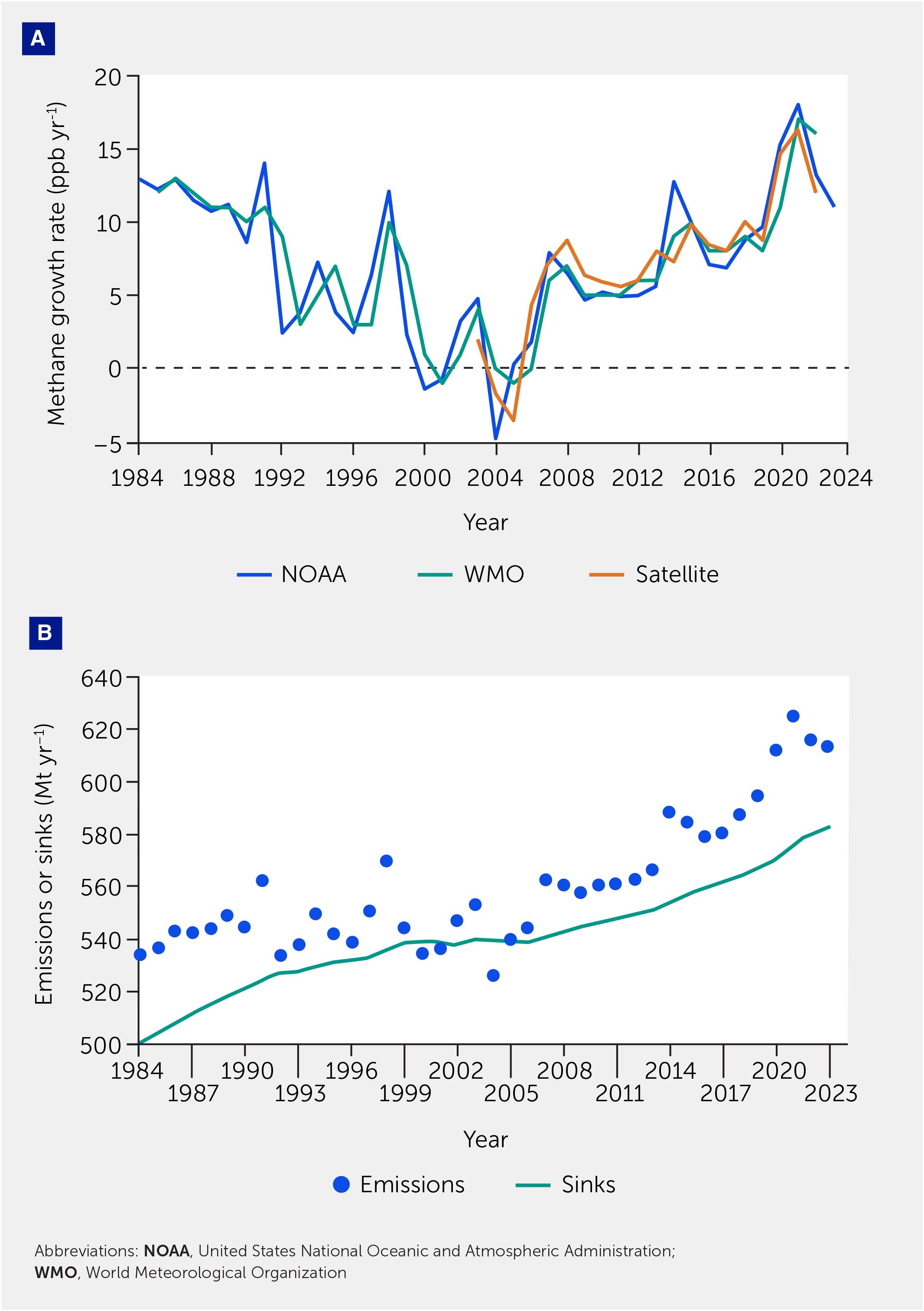
Figure 1 Accelerating methane growth rates and emissions over recent decades. (A) Observed methane annual growth rates (ppb yr−1) through 2022 or 2023 from the ground-based networks of the United States National Oceanic and Atmospheric Administration (NOAA) (9) and the World Meteorological Organization (10) and from satellite data from the Copernicus Atmospheric Monitoring Service (CAMS) (11) total column datasets. (B) Estimated emissions and sinks through 2023 based on the NOAA abundance observations. Emissions and sinks estimates are based on a simple box model assuming sinks are proportional to the atmospheric abundance of methane. Uncertainties in the ground-based and satellite data are around 0.5 ppb yr−1, and 3 ppb yr−1, respectively. See Methods (Analysis A) for further details. Data for this and other figures are available in Supplementary Table 1.
We compare the observed atmospheric methane growth rates with values under recent baseline scenarios developed with integrated assessment models (IAMs) in the early 2020s and “bottom-up” engineering approach models. All include data on actual developments through the period ~2018 to 2020 (13). The observed growth rates are roughly 1.5- to 2.5-fold higher than the multi-model mean baseline or bottom-up projections from 2020 to 2022 (Figure 2). The observed growth rates also exceed any individual model’s baseline projections during that period. Observed 2023 growth rates show the highest values of any individual model, well above multi-model means or bottom-up analyses. Baseline scenarios are used to analyze how additional technical, behavioral, and policy options can mitigate climate change. That real-world methane growth rates exceed baseline projections therefore indicates that policies may have to be even stronger than those in existing analyses to reach the Paris Agreement’s goals. Indeed, comparisons of observed atmospheric growth rates with those in 1.5°C-consistent scenarios (using the 2018 IPCC scenarios that did not include observations past 2017) show enormous differences (Figure 2), emphasizing how much stronger policies need to be to reach low-warming goals.
Figure 2
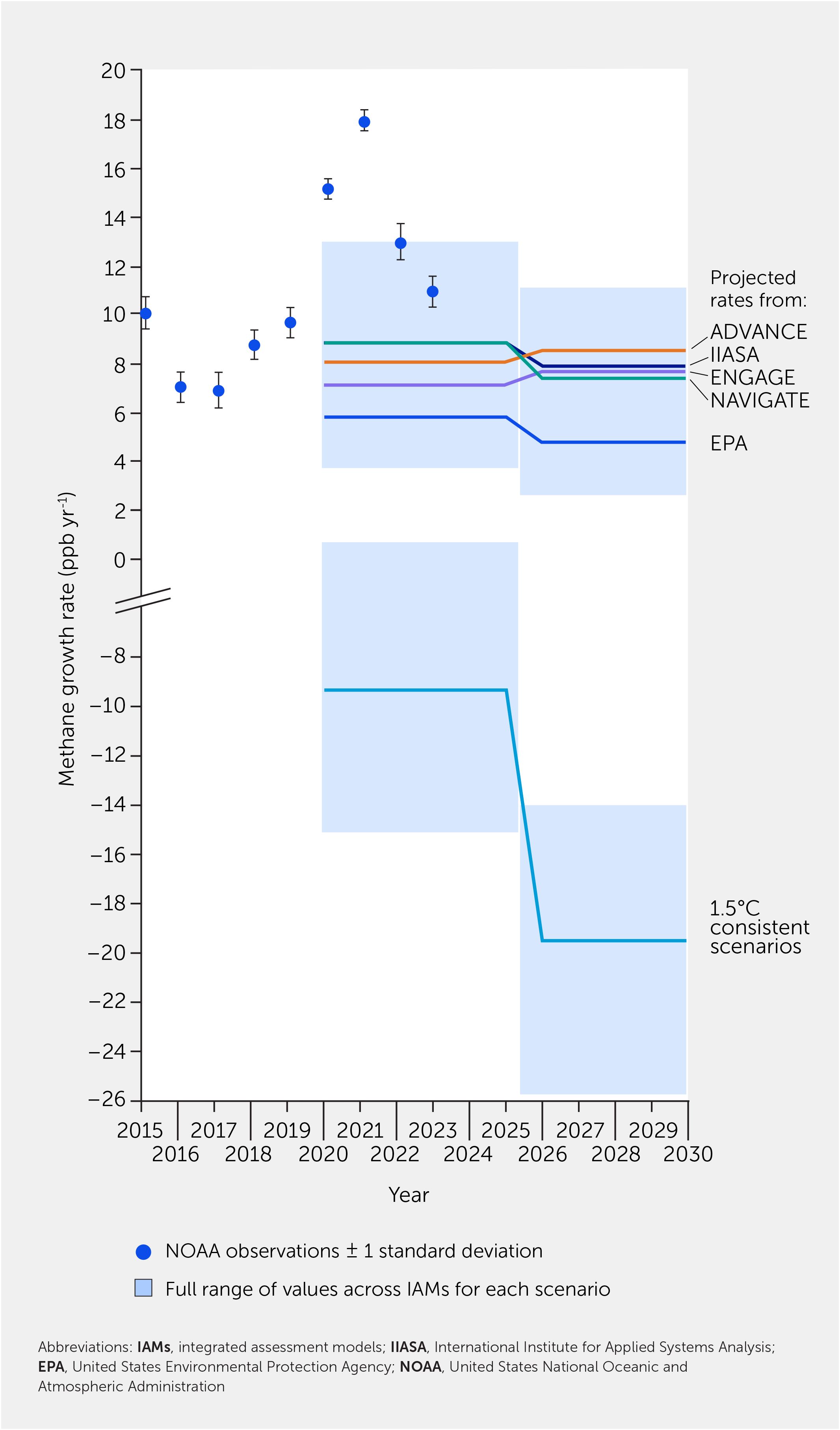
Figure 2 Projected and observed methane growth rates. Methane abundance growth rates during the 2020s from baseline scenarios from the ADVANCE (https://www.fp7-advance.eu/), NAVIGATE (https://www.navigate-h2020.eu/) (14), and ENGAGE (https://www.engage-climate.org/) projects using integrated assessment models (IAMs; data show multi-model means) and from the “bottom-up” analyses of the International Institute for Applied Systems Analysis (IIASA) (15) and the United States Environmental Protection Agency (EPA) (16) (solid lines). Modeled baseline values are averages for the 2020–2025 and 2025–2030 periods as data were produced at 5-year intervals. The shaded area shows the full range across the four to six IAMs for each scenario. Scenario concentration changes are derived from scenario emissions using a simple box model and assumed constant natural emissions of around 200 million tonnes (Mt) yr−1. Growth rates under 1.5°C-consistent scenarios with policies beginning in 2015 (17) are also shown for comparison along with their full ranges. Projected rates are compared with observations (circles) from the United States National Oceanic and Atmospheric Administration (NOAA) observation network with 1 standard deviation uncertainties. See Methods (Analysis A) for further details.
Causes of increased methane growth rates and discrepancies with baseline scenarios
Multiple assessments have concluded that the growth in methane concentrations over the 2007–2019 period is largely attributable to increased emissions from fossil fuels and livestock (18–21). However, some studies attribute much of this increase to wetlands (particularly in the tropics)—an attribution potentially supported by isotopic data indicating increased biogenic methane (22–25). In general, longer-term increases in wetland methane emissions (resulting from a human-caused warming climate) are expected to be small over these years as the climate feedback is weak according to models, modern observations, and paleoclimate data (19, 25–30). Methane emissions associated with thawing permafrost and glacial retreat are also expected to increase as the climate warms, though the magnitude is thought to be small and quite uncertain (19, 31, 32). A small portion of this longer-term increase in the growth rate may be due to growing areas of rice cultivation in Africa (33). Over the longer 2007–2019 period, there thus remains ambiguity in the cause of observed emission trends given geographical and sectorial methane source diversity.
Investigations into the cause of the large increase in the growth rate in the 2020–2023 period relative to the prior years are just beginning. Some atmospheric-chemistry transport modeling studies have attributed more than half of the increased growth in 2020 relative to 2019 to changes in methane removal owing to a decline in the hydroxyl radical OH driven by COVID-19-related changes in emissions, primarily decreases in nitrogen oxides (34–36). However, other changes that constrain methane removal rates using methane observations attribute just 14–34% of the increased 2020 growth rate to changes in the sink (37, 38). The persistence of the very high growth rates in 2021 and 2022 also supports evidence of the role of reductions in OH and methane loss rates driven by COVID-19-related emissions changes. This is consistent with Feng et al. (38), who found the role of sink changes decreased from ~34% in 2020 to just 10% in 2021. Thus, changes in methane removal appear unlikely to play a dominant role in driving the higher 2020–2023 growth rates.
Sink changes playing a minor role implies that the jump in the growth rate from 7 to 10 ppb yr−1 during the 2015–2019 period to ~12–18 ppb yr−1 during the 2020–2023 period is attributable to increased emissions, which can be examined using “bottom-up” analyses. Emission increases are unlikely to be attributable to the waste or agriculture sectors, which vary minimally from year to year. For example, global cattle numbers grew at an average rate of 1.1% yr−1 over the 2020–2022 period; this was only modestly larger than the 0.9% yr−1 average over the 2015–2019 period (39). This translates to an increase of <1 Tg yr−1 assuming constant methane emissions per animal, a small fraction of the implied emissions increase (Figure 1B) (and in contrast to the longer-term growth in cattle numbers which leads to an increase of ~10 Tg yr−1 over the 2007–2019 period). The more rapid growth of atmospheric methane over the 2020–2023 period therefore appears to be primarily linked to increased emissions from fossil fuels and wetlands, which together may account for the underestimated growth rates in the IAMs (Figure 2).
For fossil fuels, there is evidence that investments in midstream capacity have been inadequate to keep up with the volume of extracted gas as firms ramp up production. For instance, the state-owned oil company in Mexico flared ~63 billion cubic feet of gas from a single field (Ixachi) over the 2020–2022 period, representing more than 30% of the field’s total production and being in violation of Mexican law (40). Flaring to mitigate methane release is imperfect in the field: aerial measurements over multiple United States oil and gas regions indicate an efficiency of around 91% owing to both incomplete combustion and unlit flares, which, combined with large volumes of flared gas due to midstream capacity shortages, results in large methane emissions (41, 42). Studies report inefficient or inactive flares in other regions, such as Turkmenistan (43).
Additionally, some projections incorporate current emissions from national reporting, whereas studies using atmospheric inversions from satellite data suggest that oil- and gas-extracting countries in central Asia and the Persian Gulf region typically systematically underreport their emissions (44). This is similar to findings for the United States and Canada (45, 46). National reporting also generally omits so-called super-emitters (47–49), which are discussed further below. Large underestimates in initial methane emissions could lead to underestimated emission growth. Discrete events may have also played a role, with the COVID-19 pandemic being linked to increased methane emissions from the energy sector in early 2020 (50) and the 2022 Russian invasion of Ukraine causing increased efforts to expand supplies of gas and coal (51). There are thus several reasons fossil fuel emissions might be growing faster than in baseline scenarios.
However, increased methane emissions from wetlands appear likely to have driven a larger portion of the higher 2020–2022 growth rates based on the latitudinal gradients of growth rates and a trend toward lighter (biogenic) isotopes of atmospheric methane (52). The cause may be in part a persistent La Niña pattern that likely enhanced tropical wetland methane emissions during the 2020–2022 period. The wetland methane increase has been estimated at ~4–12 million tonnes (Mt) yr−1 based on empirical analyses of prior events (25, 53, 54), though another study found a weaker La Niña impact on methane (55). A recent modeling study shows a rise of ~5 Mt yr−1 in the wetland methane flux for the 2020–2021 period relative to the prior 3 years (25), predominantly from tropical ecosystems and consistent with satellite studies (38). Wetlands were also implicated in earlier analyses of the 2020 growth rate increase relative to 2019 (35), with an especially large increase in emissions from Africa (37). A rise of ~5 Mt yr−1 would be a relatively modest contribution to the overall jump in emissions estimated at ~30 Mt yr−1 for the 2020–2022 period relative to the prior 5 years (Figure 1A). There are, however, substantial uncertainties in terms of tropical wetland methane emissions (56), and modeled wetland methane emissions may be biased substantially low, especially over Africa (57, 58), so the increase shown in the models may be an underestimate. The La Niña is superimposed on anthropogenic warming and changes in climate extremes that could also lead to higher wetland methane fluxes than in previous La Niña events.
A switch from La Niña to El Niño during 2023 appears to have reduced the observed growth rate (Figure 2), supporting a large role for wetland responses to La Niña in the very high 2020–2022 growth rates. However, emissions appear to have remained substantially higher in 2023 relative to pre-2020 values (Figure 1B), suggesting longer-term contributions from increasing anthropogenic sources along with a forced trend in natural sources. Recent work also suggests a potentially permanent shift to an altered state of enhanced wetland methane emissions (8). The next 5–10 years of monitoring will, therefore, be critical in understanding both short- and long-term feedback and drivers of accelerated growth rates. While current estimates suggest increases in fossil fuel emissions, especially wetland methane, likely dominated the growth rate jump after 2019, reconciliation of observed growth rates with emissions inventories remains elusive. Regardless of the relative contribution of the two most probable major sources of the longer-term 2007–2023 increase in growth rates—i.e., wetland feedback from human-driven warming and human-driven emissions—the implications are identical: anthropogenic emissions must decrease more than previously expected to reach a given climate goal.
Imperative 2—to align methane and carbon dioxide mitigation
Methane and CO2 emissions targets
As methane targets are currently being set in many countries, it is important to understand how these fit within the broader climate change mitigation agenda and the push for “net zero CO2”. Least-cost 1.5°C- and 2°C-consistent scenarios require major and rapid reductions in methane alongside CO2 (4, 6, 17). For example, AR6 1.5°C scenarios with limited or no overshoot achieve net zero CO2 emissions around the middle of the century while methane emissions decrease by a mean of 35% (standard deviation: ±10%) in 2030, 46% (±8%) in 2040, and 53% (±8%) in 2050 relative to 2020 levels (Analysis B; Figure 3) (59). Global emissions targets well within these ranges, as in the Global Methane Pledge, are thus aligned with the Paris Climate Agreement. Delaying methane reductions past the timescales in 1.5°C-consistent scenarios risks higher overshoot, peak temperatures, and costs.
Figure 3
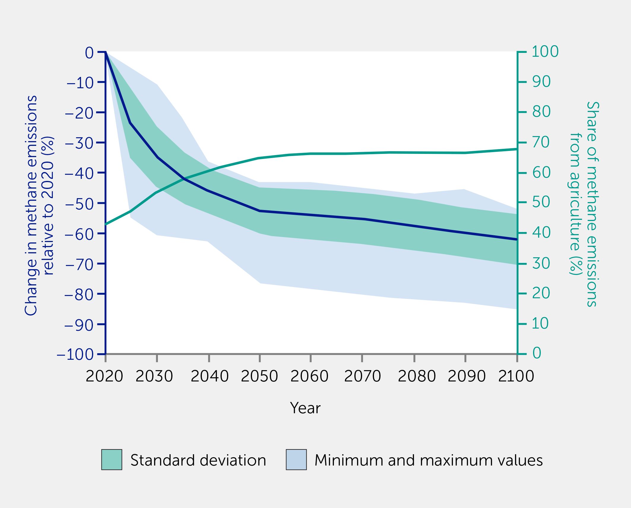
Figure 3 Decrease in total methane emissions and increase in agricultural share of the remainder in 1.5°C-consistent scenarios. Mean decrease in anthropogenic methane emissions relative to 2020 under least-cost 1.5°C consistent scenarios with policies beginning around 2020, including the standard deviation across the 53 scenarios analyzed and the maximum and minimum values across the scenarios. Also shown is the mean share of anthropogenic emissions from the agriculture sector in the same scenarios. All scenarios for which agricultural as well as total emissions were available were included (59). Note that the median scenario is virtually identical to the mean shown here. See Methods (Analysis B) for further details.
Net zero CO2 emissions is a relevant concept because options are available currently to drastically reduce CO2 in almost all emitting sectors, and carbon dioxide removal (CDR) options, including afforestation, exist for the remainder. Removal options are in the early research stages and are not currently available for methane or nitrous oxide (N2O). For those gases, we therefore discuss “zero anthropogenic emissions” (i.e., without the “net”).
The vastly different lifetimes of methane and CO2 lead to markedly different requirements for zero-emission targets. CO2, as well as other long-lived greenhouse gases (LLGHGs) such as N2O and many fluorinated gases, accumulates in the atmosphere; emissions must thus reach net zero to achieve long-term climate stabilization (17). In contrast, methane and other short-lived pollutants do not accumulate, and hence long-term climate stabilization requires only constant emissions rather than zero, with weakly decreasing emissions yielding shorter-term stabilization. Consistent with this and owing to the difficulty in reaching zero emissions in some sectors such as agriculture, none of the least-cost 1.5°C-consistent scenarios achieve zero methane (Figure 3).
Discussion of net zero GHG targets could easily be misinterpreted to imply that we can wait to reduce non-CO2 emissions since those scenarios that do achieve net zero GHGs reach net zero CO2 first. For long-term climate stabilization, the temperature depends upon the total LLGHGs emitted before reaching net zero along with the continuing short-lived pollutant emissions rate at that time, and there exists a similar relationship for peak temperatures under a peak-and-decline scenario. Article 4.1 of the Paris Climate Agreement calls for “balancing sources and removals of GHGs”, but this applies to all GHGs collectively. Achieving such a balance for methane is neither required under Article 4.1 nor for meeting the temperature goals established in Article 2 of the Agreement. In practice, methane emission projections in 1.5°C-consistent scenarios are substantial through 2100 (Figure 3). Thus, scenarios that achieve net zero GHGs accomplish this not by lowering non-CO2 emissions to zero but by aggressive deployment of CDR that offsets residual methane and N2O. This leads to gradually decreasing warming, a requirement during overshoot scenarios. Reducing warming after reaching net zero CO2 thus requires CDR, reductions of methane and/or N2O, or a combination of these. Such reductions often lead to net zero GHGs by 2100 but not always (6). This suggests that while net zero GHGs may be a laudable post-net zero CO2 goal, it might be more useful to focus separately on net LLGHG and methane targets than on net zero GHGs, which combine long- and short-lived pollutants in a metric-dependent way that obscures policy-relevant information (60) and may not be required or may be insufficient to achieve a given temperature target depending upon prior emissions.
Additionally, residual methane emissions in 1.5°C-consistent scenarios are dominated by the agricultural sector (Figure 3). A net zero GHG target that was interpreted as requiring zero methane could thus lead to conflicts between the pressure to reduce emissions from agriculture and the need to feed the world’s population. Though reducing agricultural emissions of both LLGHGs and methane is necessary and feasible (4, 61, 62), planning for net zero GHGs may lead to unrealistic expectations that could hinder progress in some countries and sectors. We, therefore, recommend that targets be formulated using net LLGHG emissions but total emission levels for short-lived pollutants.
There is an interplay between these two factors, as the higher the level at which emissions of short-lived warming pollutants remain the less total LLGHG emissions are permitted until reaching net zero to achieve a given warming level. This can be quantified using the remaining carbon budget for a particular temperature goal. To have a two-thirds chance of staying below 2°C, the remaining CO2 budget from 2020 is ~1150 GtCO2 (19), assuming roughly 35% reductions in methane by 2050. Every 100 Mt yr−1 of methane not permanently cut would take away about 300 GtCO2 from the CO2 budget over the next 50–100 years (63). This highlights the critical role of methane reductions in facilitating a plausible CO2 reduction trajectory consistent with the Paris Agreement: the remaining carbon budget would otherwise become too small to make achieving those goals feasible (64, 65).
Similarly, the more methane has been reduced upon reaching net zero CO2 emissions the less CDR would be required. For example, every additional 50 Mt yr−1 of methane permanently reduced would offset the need for ~150 Gt GtCO2 CDR over the following few decades [and >200 Gt GtCO2 over the longer term (66)]. Given the many challenges and potential negative impacts of CDR (19, 67, 68), this continues to motivate us to pursue the greatest possible methane reductions.
Measuring progress: methane and CO2 metrics
In addition to setting sound targets, it is important to use appropriate metrics to measure progress. Evaluations typically use so-called “CO2-equivalence” (CO2e), which combines all gases using the global warming potential (GWP) at a fixed time horizon, generally 100 years [e.g., (66)]. Using any single timescale to compare short-lived pollutants and LLGHGs provides an incomplete picture [e.g., (69)]. More complete climate information is gained by using multiple timescales (70, 71), among other means.
A new metric, GWP*, represents the differing effects of changes in short- and long-lived emissions on future global mean temperatures better than GWP (72). As such, the GWP* metric captures the 50–100-year relationship between continued methane emissions and the carbon budget. Hence, GWP* can be useful when examining decadal-century scale temperature changes, though multiple metrics better reflect the multiple timescales of potential interest. GWP* is applied to sustained changes in emissions, requiring careful consideration of the fact that every tonne of methane emission that persists decreases the remaining carbon budget.
One could evaluate the contribution of emissions relative to preindustrial levels using GWP*, which would show the large warming impact of present-day methane emissions (60). However, some countries and companies have used GWP* to suggest that since keeping current methane emissions constant does not add additional future warming, continued constant high levels of methane emissions are therefore not problematic and a reduction of their methane emissions is equivalent to CO2 removal [e.g., (73–75)]. This use of GWP* to justify the continuance of current emission levels essentially ignores emissions responsible for roughly half the warming to date and appears to exempt current high methane emitters from mitigation. This is neither equitable nor consistent with keeping carbon budgets within reach. Many current high emitters are wealthy groups, and the use of GWP* to evaluate changes relative to current levels implies the wealthy consuming or profiting from a large amount of methane-emitting products (such as gas, oil, or cattle-based foods) has no impact, whereas the poor, who currently consume little, would be penalized for consuming more (76). Policymakers should also consider impacts beyond climate when choosing policies affecting methane (4, 77–79).
Connections between methane and CO2 mitigation options
Though the different lifetimes of methane and CO2 have profound implications for target setting and metrics, the separation between short- and long-lived pollutants is not complete. Much like other short-lived pollutants, methane induces climate changes that affect the carbon cycle—thereby exerting a long-term impact (80, 81). This carbon-cycle response to warming adds ~5% to the forcing attributable to methane emissions. Additionally, methane emissions lead to increased surface ozone, which is harmful to many plants and reduces terrestrial carbon uptake. Climate impacts of methane emissions could be increased by up to 10% considering ozone–vegetation interactions (12).
In addition to these Earth system interactions, mitigation options also link methane and CO2. Decarbonization policies phasing out fossil fuels would clearly reduce fossil sector methane emissions. However, those reductions would produce only about one-third of the methane reductions in 1.5°C scenarios by 2030 (4, 82). The use of non-fossil methane sources for energy production also modestly reduces CO2 emissions by displacing demand for fossil fuels, adding ~10% to the long-term and ~3% to the near-term climate effect of methane capture. Other estimates suggest that using non-fossil methane for power generation could increase the monetized environmental benefits of methane capture even further—by 14% and 25% for discount rates of 4% and 10%, respectively. These larger values reflect the inclusion of both climate and air pollution damages and stem primarily from reduced air pollutants associated with coal burning (78).
Another intersection between decarbonization and methane could occur in a hydrogen economy. Fugitive methane emission rates above ~2% would cancel the near-term climate benefits of “blue hydrogen” with carbon capture and sequestration (CCS) compared to burning natural gas (83). Furthermore, hydrogen leakage would extend methane’s lifetime by lowering the atmospheric oxidative capacity [e.g., (84, 85)].
Land use also links mitigation options for methane and CO2. There are large land area requirements for either bioenergy with CCS (BECCS) or afforestation, two sources of CDR that most low-warming scenarios require to compensate for slow decarbonization and/or continued emissions from the sectors most difficult to decarbonize (17). Given the demands on arable land to feed a growing population and the urgent need to restore and conserve biodiversity, a plausible source of additional land is reduced numbers of pasture-raised livestock, which could also reduce methane emissions.
To probe this connection, we examined 145 least-cost 1.5°C scenarios for which trends in pasture area and BECCS deployment were available (Analysis C) (86). The deployment of BECCS closely mirrors a decline in pasture area in these scenarios (Figure 4A), a relationship noted but not quantified in AR6 (59). Examining the multi-model mean decadal changes from the 2040s onwards, when deployment of BECCS is large enough to show clear trends, we find highly correlated changes, with every 10 exajoule (EJ) of BECCS associated with ~38 million ha pasture area decrease (Figure 4B) and ~0.5 Gt yr−1 CO2 removal. Adding in the 2030s increases the slope to 42 million ha per 10 EJ, whereas examining each individual scenario’s changes, rather than the multi-model mean, shows the slope is 28 million ha per 10 EJ. These comparisons give a sense of the robustness associated with this relationship.
Figure 4
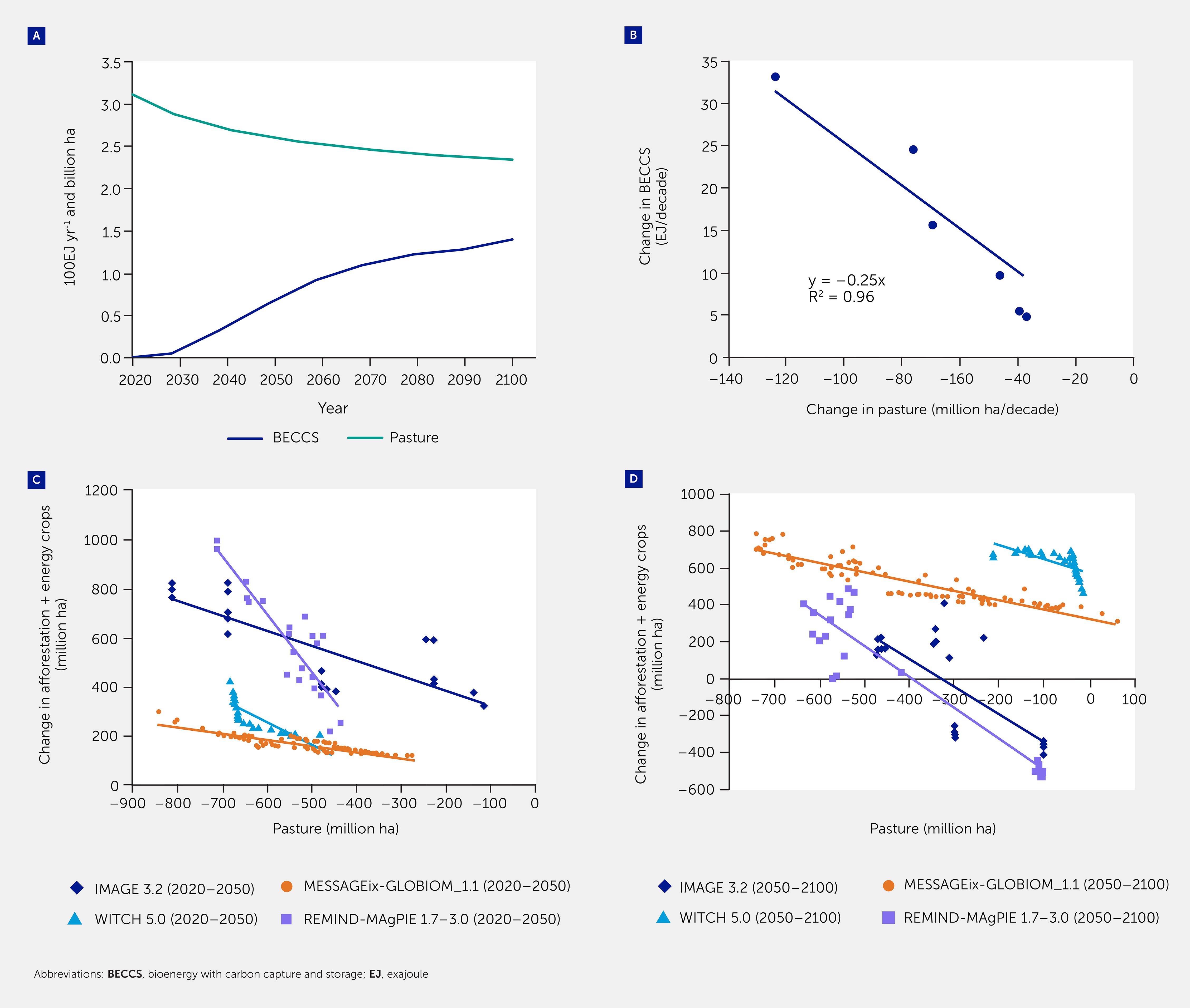
Figure 4 Trade-offs between land use for pasture and for carbon uptake. (A) Multi-model mean trends in bioenergy with carbon capture and storage (BECCS) deployment and in pasture area in the 145 available least-cost 1.5°C scenarios. (B) Correlation between decadal changes in the multi-model means of these two quantities from the 2040s to 2090s. Data are from seven integrated assessment models (IAMs) from the 2022 AR6 scenario database (86). Also shown are land use changes from simulations covering 22–106 <2°C scenarios per model in individual IAMs for 2020–2050 (C) and 2050–2100 (D), including linear trend estimates across the scenarios. See Methods (Analysis C) for further details.
For reforestation and afforestation, meeting goals in national climate pledges is projected to require almost 1.2 billion ha of land (87). For context, the current crop area is about 1.2 billion ha (including animal fodder), so changes in land used for crops for humans would be too small to provide the land needed while maintaining food security. While some land needs might be met via restoration of degraded lands, more than half was estimated to require conversion of pasture or land currently used for animal fodder.
To evaluate the relationship between afforestation plus biofuel land use and pasture, we examined a larger AR6 set of scenarios that keep warming below 2°C, finding 266 scenarios (Analysis C). Averaged across the models, pasture area decreases by 1.1 ha per 1 ha land used for carbon uptake from 2020–2050 and by 0.6 ha from 2050–2100. Assuming carbon uptake per ha biofuel crops is similar to afforestation, this corresponds to ~94 million and 54 million ha of pasture required per GtCO2 removal, with a range of 28–251 million ha across the models. This range encompasses the results based on BECCS alone in the 1.5°C scenarios. Together, these analyses show robust evidence of a tradeoff between land used for CDR and pasture with a value that is highly model-dependent. In the four models including afforestation, changes in land deployed for carbon uptake are highly correlated with pasture decreases across the scenarios, with R2>0.6 and 0.4 for 2020–2050 and 2050–2100, respectively (Figures 4C, D). Within the IAMs, MESSAGE and REMIND show fairly linear relationships whereas the land use tradeoff is more dependent on the scenario in WITCH and IMAGE (Figures 4C, D). Land for CDR is used primarily for BECCS in MESSAGE and WITCH, primarily for afforestation in IMAGE, and comparably for those options in REMIND, highlighting that the tradeoff with pasture holds for all uptake options deployed in the models. Inter-model differences presumably stem from varying assumptions about the availability of non-agricultural land for afforestation, changes in non-energy crop area, and the intensity of carbon uptake via afforestation or energy crops.
The results show that shifting livestock practices, especially healthier dietary choices that in many places lead to reduced consumption of cattle-based foods and hence decreased livestock numbers, not only affect methane emissions but are also tightly coupled with CDR strategies (88). Both current pledges for biological carbon removal and BECCS deployment at the scales envisioned in many scenarios likely require large reductions in pasture area, and dietary changes could free up pasture without risking food security. We note that both biological carbon removal and BECCS come with substantial challenges and side effects that affect the likelihood that they will ever be societally acceptable at scale (19, 87).
In summary, reductions in methane emissions are not just complementary to CO2 reductions but can directly contribute to reduced atmospheric CO2 via carbon cycle interactions and fossil fuel displacement. They can also potentially play an important role in facilitating the deployment of, as well as reducing the need for, CDR; this could reduce additional feedback, including increased volatile biogenic compound emissions following afforestation that might increase methane’s lifetime (89).
Impacts of methane and carbon dioxide mitigation
As noted, methane emissions are estimated to account for 0.5°C of the total observed warming of 1.07°C through the 2010–2019 period (1). As the climate is affected by both warming and cooling pollutants, the attribution of the fraction of observed warming to a specific component depends on which drivers are included in the comparison. Compared with the total observed warming, methane emissions are responsible for ~47% of that value; in comparison with the warming attributable to all well-mixed GHGs, methane emissions are responsible for ~34%; and in comparison with the temperature increase due to all warming agents, methane emissions contribute ~28%. As the overlap between methane sources and other climate drivers is relatively limited, methane could potentially be reduced with only modest effects on other emissions. Comparison with observed net warming may therefore be most useful, but each of these comparisons is useful for specific purposes. To prevent public confusion, presentations that imply methane’s contribution is being evaluated against observed warming when it is not and that do not state if they are referring to emissions or concentrations, such as the common statement that methane is responsible for around 30% of global warming since pre-industrial times [e.g., (90, 91)], should be avoided. Note also that the share of warming attributable to a given driver varies depending upon the baseline period (1850–1900 in AR6).
Emission reduction policies that target methane and CO2 have complementary and additive benefits for the climate. We analyzed the response of global mean annual average surface air temperatures to emissions under various scenarios to isolate the effects of decarbonization and targeted methane emission controls (Analysis D). Contemporaneous reductions in cooling aerosols associated with decarbonization lead to modest net warming over the first few decades [e.g., (13, 92–95)]. Given the smaller role of other non-CO2 climate pollutants, methane emission cuts therefore provide the strongest leverage for near-term warming reduction (Figure 5) (13, 95). Achievement of methane reductions consistent with the average in 1.5°C scenarios could reduce warming by ~0.3°C by 2050 in comparison with baseline increases (4). A hypothetical complete elimination of anthropogenic methane emissions could avert up to 1°C of warming by 2050 relative to the high emissions Shared Socioeconomic Pathway [SSP; (96)] SSP3–7.0 scenario (97). This large near-term impact partly reflects methane’s short lifetime; >90% of increased atmospheric methane would be removed within 30 years of an abrupt cessation of anthropogenic emissions compared with only ~25% of increased CO2 following CO2 emission cessation (98). Encouragingly, were humanity to abruptly cease emissions, the present combined anthropogenic CO2 and methane concentration increases versus preindustrial [weighted by their warming contributions, including the ozone response to methane (12)] levels would be halved within 30 years. Hence the near-term “Zero Emissions Commitment” of warming already “in the pipeline” (19, 99) is much smaller considering both methane and CO2 rather than CO2 alone.
Figure 5

Figure 5 Climate impacts of decarbonization and methane reductions. The climate response (measured by change in global mean surface temperature relative to 2020 values) to reductions of all pollutants (including methane) under a decarbonization scenario; methane alone under a decarbonization scenario that substantially reduces energy sector emissions and under a 1.5°C scenario; and decarbonization and methane reductions consistent with 1.5°C—all relative to constant 2020 emissions. Values are averages across Shared Socioeconomic Pathways (SSPs) 1, 2, and 5 (1.5°C was infeasible under SSP3 in four of four models and under SSP4 in two of three models). See Methods (Analysis D) for further details.
Policies leading to rapid and deep cuts in both CO2 and methane provide the strongest benefits across the century (Figures 5; 6A). To further characterize the relative contributions, we analyzed temperature responses, and their effects on premature mortality, applied to various mitigation options under the “middle-of-the-road” SSP2 (Analysis E). Importantly, future CO2 emissions exert the strongest leverage on long-term climate change, and successfully targeted methane reduction without simultaneous CO2 reductions over the next 10–30 years would therefore merely delay long-term warming (Figure 6A). Conversely, successful reduction of CO2 (and co-emissions) without simultaneous additional targeted methane reduction over this period would weakly affect long-term temperatures if methane reductions were achieved later (Figure 6A) but would lead to higher warming and substantially increased risk of overshooting warming thresholds over the next few decades. In addition to the impacts on warming, a 20-year delay in methane reductions from 2020 to 2040 would also lead to 4.2 (1.3–6.8; 95% confidence) million additional premature deaths due to ozone exposure by 2050 that could have been avoided with rapid methane reductions based on our standard epidemiological estimates (Figure 6B). That value becomes ~8.8 (5.5–11.1) million additional deaths using alternative cardiovascular and additional child-mortality relationships (Analysis E).
Figure 6
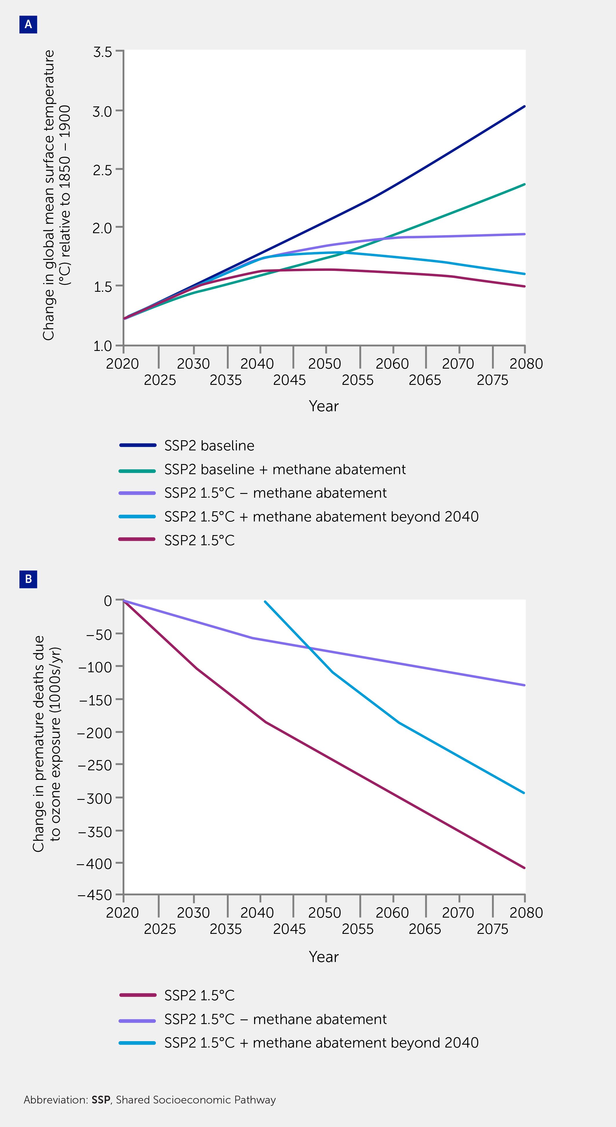
Figure 6 Temperature and health impacts of methane abatement under various scenarios. (A) Climate response (measured by change in global mean surface temperature relative to 1850–1900 values) to all pollutants under the baseline Shared Socioeconomic Pathway (SSP) 2 scenario; the SSP2 baseline plus methane abatement consistent with a 1.5°C scenario; the SSP2 1.5°C scenario (SSP2–1.9); the SSP2 1.5°C scenario without any additional methane abatement beyond that occurring due to the phase-out of fossil fuels; and the SSP2 1.5°C scenario with additional methane abatement beyond that occurring due to the phase-out of fossil fuels beginning in 2040 rather than 2020. (B) Avoided premature deaths resulting from methane reductions relative to those under the SSP2 baseline (note that SSP2 baseline plus methane abatement consistent with a 1.5°C scenario is identical to the SSP2 1.5°C scenario for this impact and so is not shown). See Methods (Analysis E) for further details.
In addition to reducing early deaths, cutting methane emissions will reduce near-term warming impacts on labor, which grow non-linearly with warming (100). We used our climate Analysis E as the basis to estimate corresponding labor effects of changing heat exposure (Analysis F). Assuming outdoor workers are in the shade, achieving 1.5°C-consistent methane abatement under SSP2 avoids roughly US$250 billion in worldwide potential heavy outdoor labor losses by 2050 (range US$190–US$390 over impact functions; values in 2017 US$ purchasing power parity). However, for outdoor workers in the sun, benefits would be roughly US$315 billion (range US$211–US$475). These values, for heavy outdoor labor only, are not comparable to impacts covering medium and light labor (for which the evidence base is weaker).
Imperative 3—to optimize methane abatement options and policies
Global context
Despite substantial uncertainties in emissions from specific subsectors, global-scale anthropogenic methane emissions are reasonably well-constrained. Agriculture and fossil fuel emissions have comparable magnitudes (each ~130–150 Mt yr−1) roughly twice that of the waste sector (~70–75 Mt yr−1) (4, 101). Abatement technologies are available in each sector (102) and, with modest projected improvements over time, could provide reductions of 29–62 Mt yr−1 in the oil and gas subsectors together, 12–25 Mt yr−1 in the coal subsector, 29–36 Mt yr−1 in the waste sector, and 6–9 Mt yr−1 from rice cultivation in 2030 (4, 90). Estimated abatement for livestock ranges from 4–42 Mt yr−1, depending upon factors such as the assumed potential to adopt higher productivity breeds and/or reduce total animal numbers. Technical abatement could be enhanced with nascent technologies such as methane inhibitors for ruminants, cultured and alternative proteins, and, in the waste sector, biocovers, black soldier flies, and waste-to-plastic substitute systems.
Many technological abatement options capture concentrated flows of methane, allowing it to be used as natural gas, generating revenue that lowers net costs. Defining low-cost as <US$600 per tonne of methane (in 2018 US$), low-cost abatement potentials represent 60–98% of the total for oil/gas, 55–98% for coal, and ~30–60% for waste (4, 89). Technical options with net negative costs could reduce total emissions by ~40 Mt yr−1, with the greatest potential being in the oil/gas and waste sectors (4).
Systemic and behavioral choices, such as fuel switching and demand management, also affect methane emissions and are particularly important in the food sector. Cattle account for about 70% of livestock emissions, with ~25% from regions with high reliance on intensive systems (primarily Europe and North America) most suitable for technical solutions (15). In other areas, extensive grazing systems are common, limiting technical solutions (61). For sizeable reductions in livestock emissions, cuts in animal stocks will therefore be necessary. Shifts to more plant-based diets could bring health benefits in regions with high intake of animal protein (103, 104), and, as discussed above, this is important for providing areas for CDR deployment. Such shifts could reduce methane emissions by ~15–30 Mt yr−1 over the coming ~10–25 years (4). In regions with low protein intake but large cattle herds, productivity should be increased in conjunction with enhancement of the economic resilience of pastoralist communities (105). The latter requires improved access to affordable healthcare, education, and credit markets to enable management of financial risks without reliance on large livestock herds.
Achieving ~40–50% reductions in food loss and waste could reduce ~20 Mt yr−1 of methane emissions (4). Systemic and behavioral changes, such as dietary shifts and reduced food loss/waste (DFLW), are often difficult to implement but are benefiting from growing attention. Together, these could substantially augment the 120 Mt yr−1 achievable through targeted technical controls (13, 62, 106). Similarly, the IPCC assessment indicates a mitigation potential from DFLW for all GHGs of about 7 (3–15; full range) GtCO2e yr−1 by 2050, of which 1.9 GtCO2e yr−1 comes from direct emissions [largely non-CO2 (6)]. The latter would correspond to ~70 Mt yr−1 methane were it all methane, highlighting the large mitigation potential from DFLW both via methane and via associated land use changes.
National mitigation options: abatement potential and cost-effectiveness by country
The GMP has raised ambition worldwide but achieving its goal requires optimizing efforts, as political and financial capital is limited and time is short. We have therefore undertaken national-level analyses (Analyses G–H) of technical mitigation options for countries seeking to implement the Pledge or non-signatories that may want to reduce their emissions (e.g., China published a National Methane Emissions Control Action Plan in 2023). These analyses may also help optimize international financing. They are based on data from the United States Environmental Protection Agency (EPA) (16) and the International Energy Agency (IEA) (90).
Mitigation options with greatest abatement potential by country
Analyses of technological mitigation potential highlight the need to address all subsectors given that each is the largest in at least some countries (Analysis G; Figure 7). In some fossil-fuel-producing countries, the greatest opportunities for methane mitigation are in gas and oil whereas coal predominates in other countries. Despite substantial fossil fuel industries, several countries in the Middle East, Southern Africa, and South America are estimated to have their largest mitigation potential in landfills. With few fossil fuels produced outside Eastern Europe and limited technical mitigation potential for livestock, the largest potential for mitigation in Europe is also often in landfills. There are notable exceptions, however. In France, Germany, and the Nordic countries, for example, policies have greatly mitigated waste sector emission, and the livestock subsector now has the largest remaining mitigation potential. This illustrates how national-level data reveal substantial variations even within relatively small geographic regions.
Figure 7
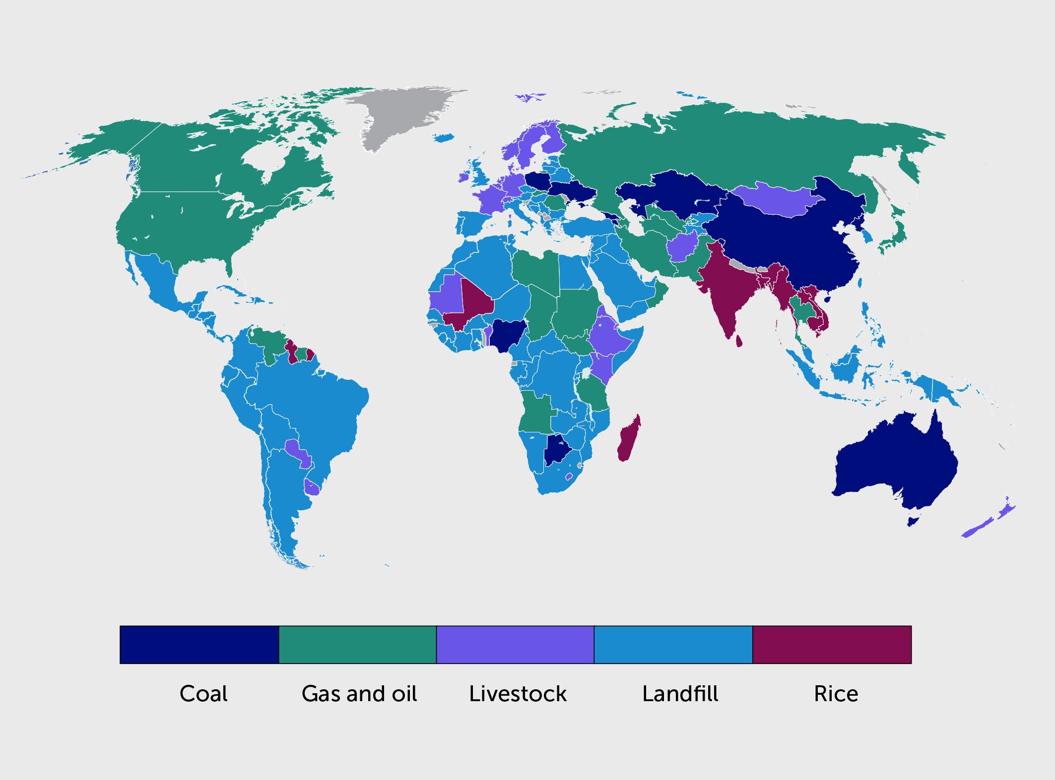
Figure 7 The subsector with the largest technical mitigation potential in every country. The map shows the subsector with the greatest mitigation potential regardless of the cost in each country based on United States Environmental Protection Agency (EPA) data (16). See Methods (Analysis G) for further details.
This analysis is based on bottom-up emission estimates relying on activity data combined with emission factors. This is the most detailed emission information available by subsector for all countries. However, this approach has uncertainties and limitations. Recent developments in satellite remote sensing have shown the existence of so-called “super-emitters” (48, 49, 107). These are facilities emitting enormous amounts of methane, often related to abnormal operating conditions such as gas well blowouts (108) or non-burning flares. Hundreds of super-emitters are detectable globally, with even more at local scales [e.g., (47)]. Many super-emitters can be considered “low-hanging fruit” since they are especially cost-effective to mitigate and have high reduction potential per individual source, making them a high-priority category to address. However, they are often not well represented in bottom-up inventories and do not necessarily follow the prioritization per country suggested by the bottom-up analysis (Figure 7). For example, satellite-based studies show emissions from super-emitters from the oil and gas industry in Algeria of ~100 kt CH4 yr−1 (48, 49), a substantial fraction of the estimated mitigation potential not including super-emitters (Figure 8A). Super-emitters have also been reported in the coal subsector in Australia, China, and the United States (108–110). Urban areas are also important emission sources that can be difficult to capture in inventories with >13 urban methane hotspots detected in India (49) and evidence of worldwide urban wastewater emissions hotspots (111). Based on high-resolution satellite observations, individual landfills in New Delhi and Mumbai were estimated to emit 23 (14–33) and 86 (53–228) kt CH4 yr−1 (112), a large fraction of total emissions from their respective urban areas.
Figure 8
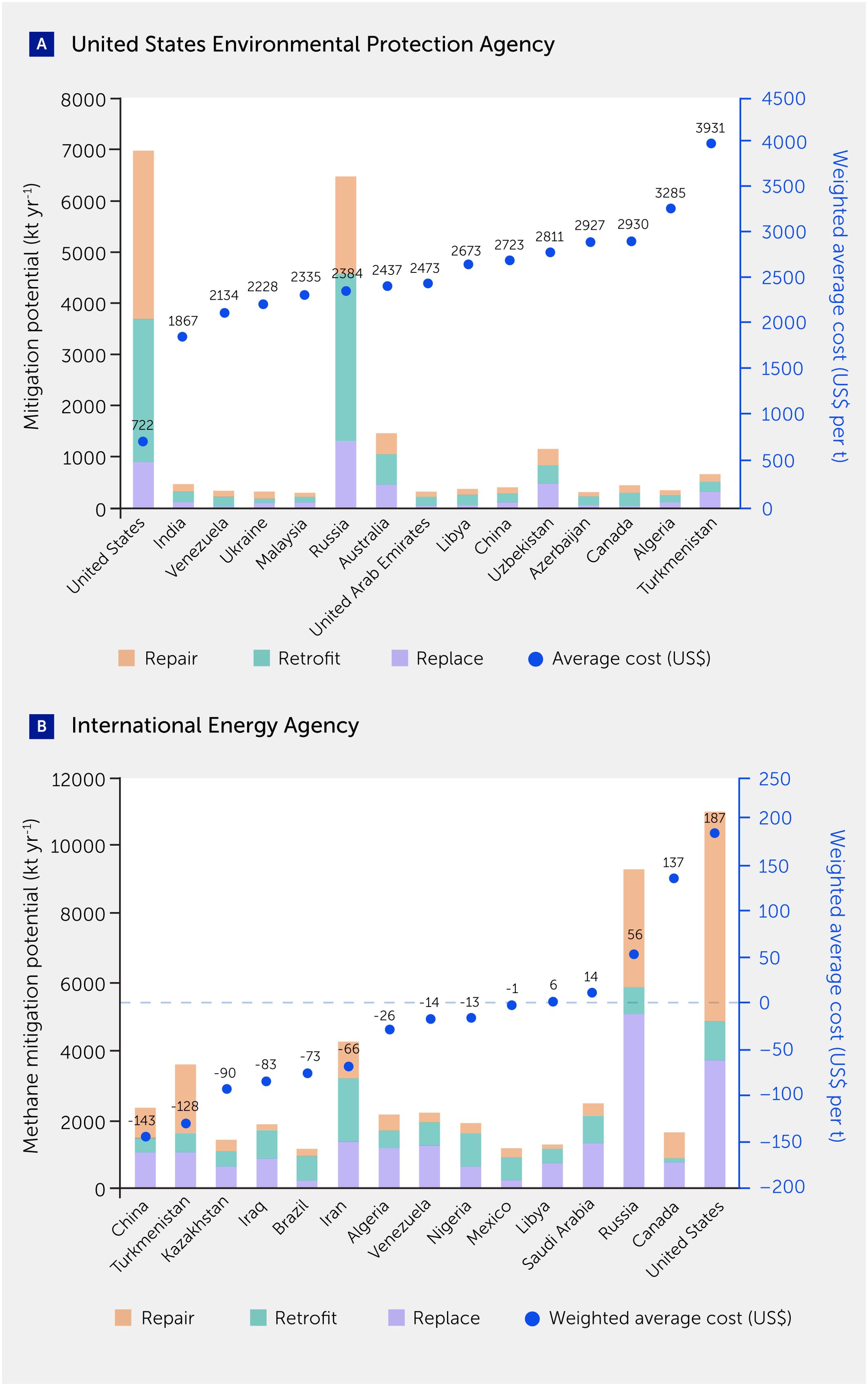
Figure 8 Favorable countries for mitigation of methane from the oil and gas subsector. Estimated methane mitigation potential and costs within the oil and gas subsector for the 15 countries with the greatest mitigation potential in this subsector regardless of costs. Analyses based on data from (A) the United States Environmental Protection Agency (EPA) for 2030 (16) and (B) the International Energy Agency (IEA) for 2022 (90). See Methods (Analysis H) for further details.
Mitigation potential and cost-effectiveness by sector and country
To explore cost-effectiveness, we focus on the 50 countries with the largest subsector mitigation potential in the next decade and then rank those by abatement costs (Analysis H). This excludes the agricultural sector due to the limited potential for technical solutions to achieve sizable reductions in the short term. Although this analysis highlights the nations with the largest mitigation potentials at the least average cost, costs vary within each subsector. We therefore created an online tool to explore such details (https://github.com/psadavarte/Methane_mitigation_webtool). Mitigation options are grouped into functionally similar categories to facilitate readability and allow comparison across estimates (Table 1).
Table 1
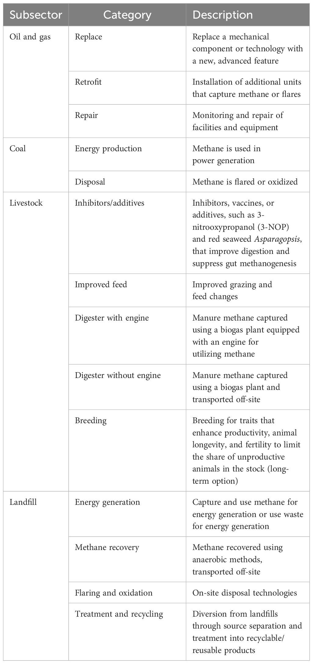
Table 1 Technical mitigation options included in each category.
Landfills
For landfills, the 15 most cost-effective large reductions total >6 Mt yr−1, and all have net negative costs (Figure 9). These savings result from revenues provided by methane recovery for use offsite or energy generation. Within these two categories, net mitigation costs range from −US$800 to −US$4400 per tonne. The mitigation potential is always the largest in the energy generation category, hence savings outweigh expenses from flaring and oxidation (~US$120–US$330 per tonne in these countries) and waste treatment and recycling (US$400–US$1700 per tonne). Mitigation potentials are large for some countries with very large populations, such as India, Brazil, and Mexico, but also for several countries with smaller populations including Azerbaijan, Poland, Peru, and the United Arab Emirates. Note that the most cost-effective options do not always have the greatest mitigation potential (e.g., energy generation versus organics diversion).
Figure 9
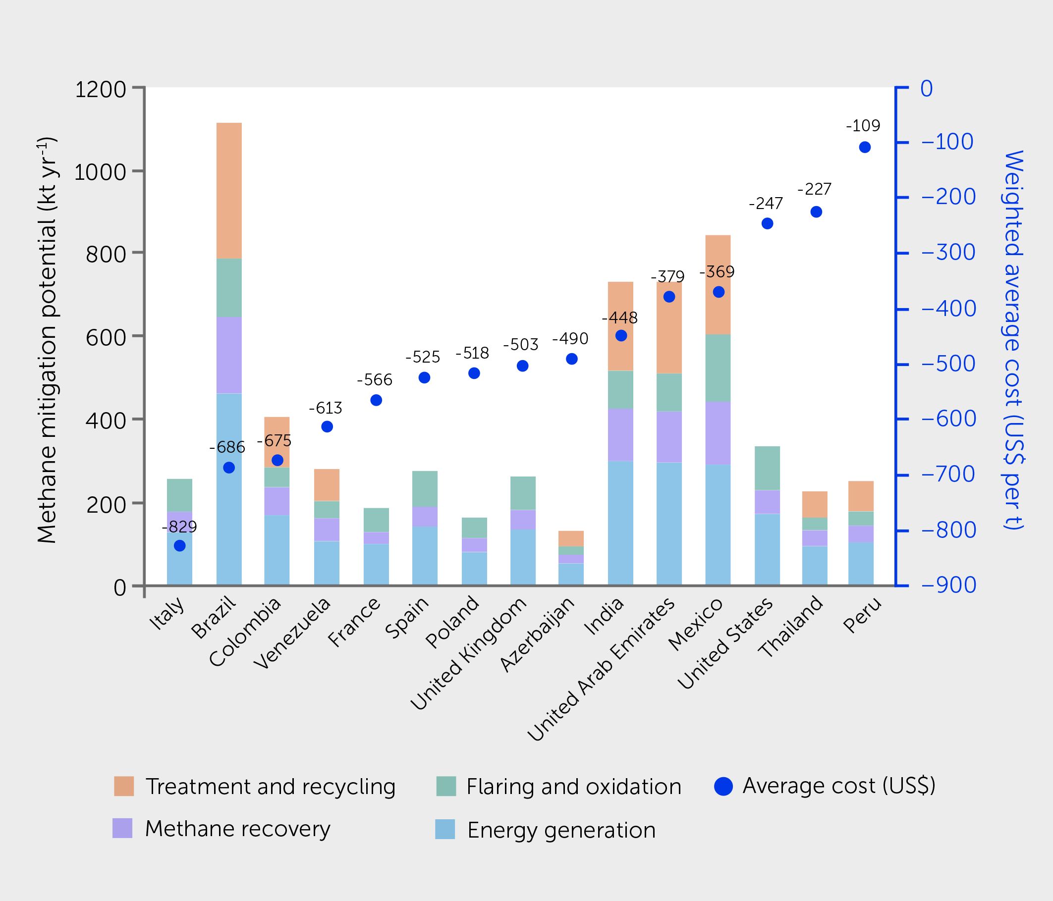
Figure 9 Favorable countries for mitigation of methane from landfills. Estimated 2030 methane mitigation potential and costs within the landfill subsector for the 15 countries with the least expensive average costs that are also among the top 50 countries for mitigation potential in this sector. Analysis based on data from the United States Environmental Protection Agency (EPA) (16). See Methods (Analysis H) for further details.
Estimating landfill mitigation potentials requires assumptions about waste diversion potentials that are difficult to constrain. For example, analyses by the International Institute for Applied Systems Analysis (IIASA) (15) for India and China find mitigation potentials ~3.5 times larger than EPA values (Table 2). In contrast, the IIASA mitigation potential for the former Soviet Union countries is smaller. Differences are related to IIASA using both population and economic growth as drivers for waste generation (EPA uses population growth only) and IIASA finding a larger mitigation potential from diversion of organic waste through recycling and energy recovery than in the EPA analysis. National-level analyses have substantially larger ranges in estimated mitigation potentials than the global totals—which are similar to the EPA and IIASA analyses. Cost differences between these analyses are even more striking (Table 2) and reflect differences in the assumed value of recycled products recovered from municipal waste and discount rates (5% for EPA, 4% for IIASA). A small number of very expensive controls in the EPA analysis also have an outsized impact. For example, screening out options costing >US$600 tCH4−1 reduces the cost averaged over the remaining measures to −US$2700 tCH4−1 for India, closer to the IIASA results.
Table 2
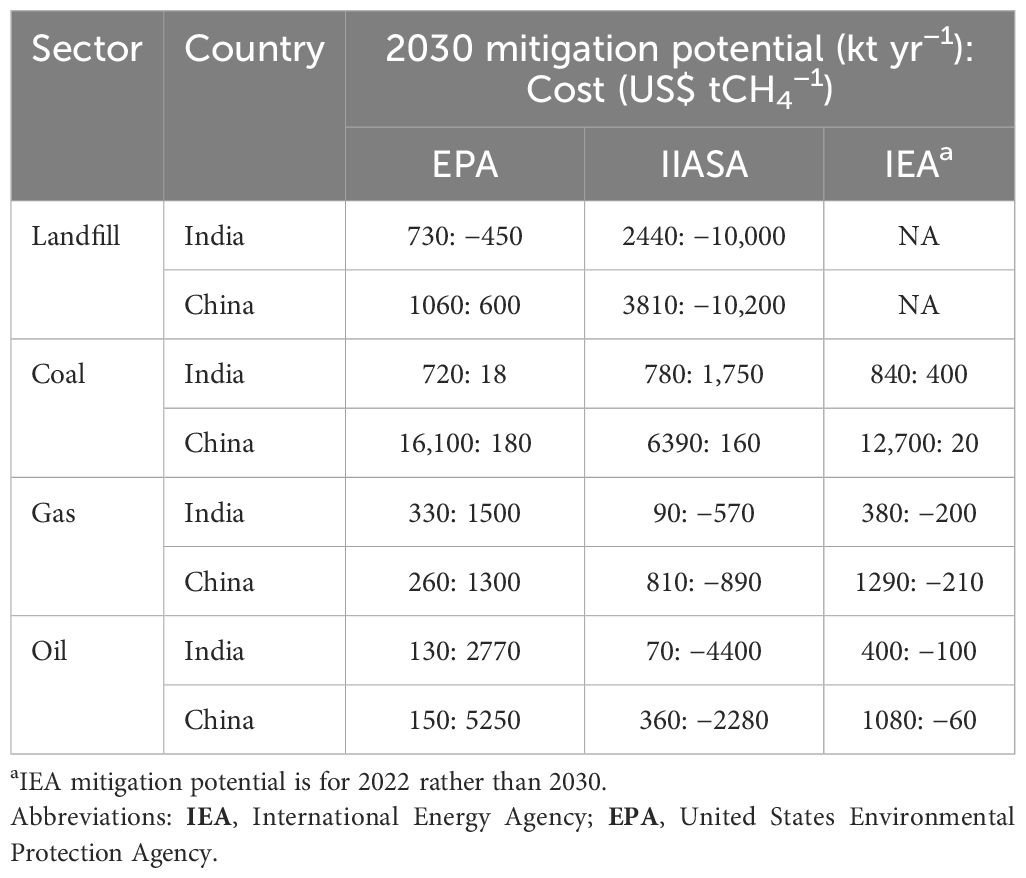
Table 2 Comparison of national data for India and China across available analyses.
Coal
For coal, nearly all the most cost-effective large national reductions have positive average costs, though they are low at <US$600 tCH4−1 for the top 15 nations (Figure 10; Table 2). Mitigation potential in coal within China provides over half the global total for the subsector in all analyses, but the EPA mitigation potential is more than double the IIASA’s, with the IEA being in between (Table 2). The EPA analysis has larger baseline methane emissions from coal in China: 26 Mt yr−1 in 2020 versus 20 and 21 Mt yr−1 in the IIASA and IEA analyses, respectively (2030 values are similar). The lower values are closer to recent satellite inversion estimates of ~16–18 Mt yr−1 (113). IIASA also makes more conservative assumptions than EPA regarding the fraction of ventilation air methane (VAM) shafts with CH4 concentration levels high enough (>0.3%) to install self-sustained VAM oxidizers. Cost estimates for China are similar between EPA and IIASA, with the IEA’s being lower. In contrast, the three estimates for coal mitigation potential in India are very similar, but cost estimates differ greatly (Table 2). IIASA’s high costs for India reflect the low VAM concentration there (<0.1%), severely limiting the applicability of oxidizers. Furthermore, abatement potentials in India are similar in magnitude but represent very different percentages of the baseline emissions, with the EPA estimate being roughly one-third that of the other analyses.
Figure 10
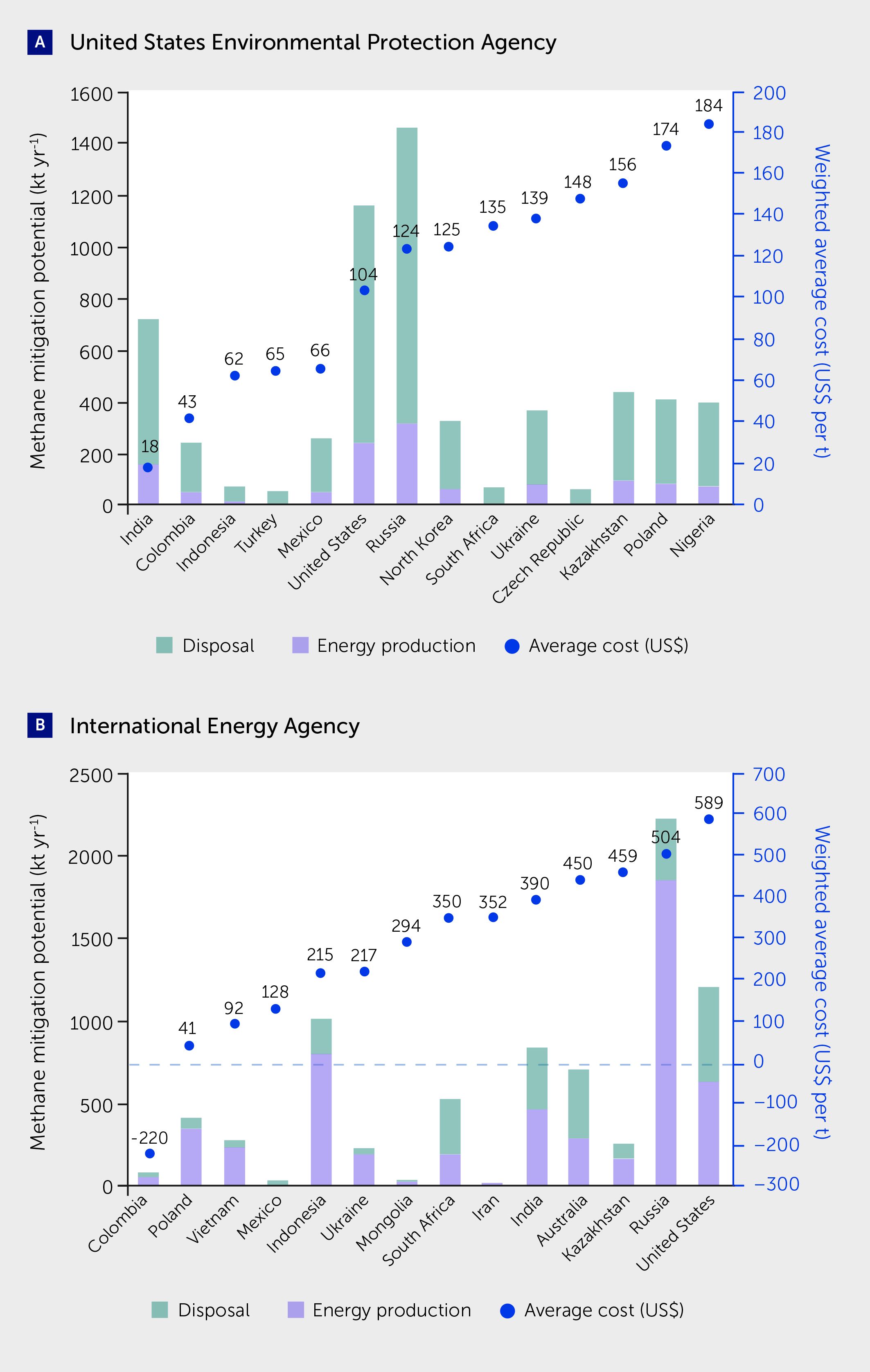
Figure 10 Favorable countries for mitigation of methane from the coal subsector. Estimated methane mitigation potential and costs within the coal subsector for the 14 countries with the least expensive average costs that are also among the top 50 countries for mitigation potential in this subsector. Analysis based on data from (A) the United States Environmental Protection Agency (EPA) for 2030 (16) and (B) the International Energy Agency (IEA) for 2022 (90). Note that China is also among the top 15 countries in both analyses but has a mitigation potential of >12,000 kt yr−1 (Table 2), far beyond the scales shown here. See Methods (Analysis H) for further details.
Generally, the EPA estimates lower costs than the IEA, but many countries have similar abatement potentials, including Russia, India, and the United States (Figure 10). In other cases, they estimate extremely different mitigation potentials, for example, in Indonesia and Australia. Differences result from multiple factors, including limited data on base costs and emissions levels, reference years, and technical and economic assumptions. For example, the contrast for Indonesia reflects differences in estimated baseline levels of emission, with the EPA indicating a much lower volume. This may be related to differences in the reference year, with the IEA estimate being more recent and reflecting higher coal activity in Indonesia. Additionally, the EPA uses lower IPCC default emission factors and country-level reporting data to estimate coal mine methane emissions, whereas the IEA considers coal rank, mine depth, satellite measurements, and regulatory frameworks. Finally, the energy production category typically has lower costs than the subsector average, and often net negative costs, whereas the disposal category does not generate revenue and so has higher costs. The latter is typically the largest component in the EPA analysis whereas the former tends to be the largest in the IEA analysis (Figure 10).
Oil and gas
Oil and gas data are available for most countries from the EPA and the IEA. We focus on the 15 countries with the largest potentials regardless of cost because these are similar sets of countries, whereas the most cost-effective within the top 50 differ greatly in these analyses. The comparison shows that 8 countries are among the top 15 by mitigation potential in both analyses, yet these differ markedly in mitigation potentials and especially in mitigation costs (Figure 8). For example, both analyses show the largest abatement potentials in the United States, followed by Russia. However, the potentials estimated by IEA are 40–50% larger than the EPA estimates, while the costs are four-fold lower for the United States and 40-fold lower for Russia. Mitigation potentials diverge even more in other countries. For instance, for Turkmenistan, the IEA finds the potential to mitigate 77% of 4700 kt yr−1 whereas the EPA finds a mitigation potential that is 37% of 1800 kt yr−1. The IEA analysis, incorporating satellite-based emissions estimates, typically estimates higher current emissions than the EPA which relies upon national reporting, accounting for the larger IEA values in several countries. However, for Uzbekistan and Russia, the IEA base emissions are much lower, at 670 and 13,600 kt yr−1, respectively, versus 3000 and 24,800 kt yr−1 in the EPA analysis (Russian official reporting was revised downward since the EPA analysis).
Differences between cost estimates are more systematic across countries, with the IEA consistently much lower than EPA. Differences are linked to several factors, including the inclusion of “super-emitters” by the IEA, a scarcity of data on required capital and operational expenditures, and varying revenue assumptions and typical lifetimes for abatement measures (the EPA uses a 5% discount rate and the IEA 10%, which would generally lead to relatively lower costs for the EPA). For example, the EPA estimates incorporate uniform natural gas prices across segments, whereas the IEA has different prices for upstream and downstream segments. Mitigation measures also vary, with each having specific costs, revenue, and lifetime in both analyses.
For both gas and oil, IIASA analyses show much smaller mitigation potential for India than either the EPA or IEA analyses, whereas for China, the IIASA estimates lie between EPA and IEA values (Table 2). For both countries, mitigation potentials vary by 300% to 600% across the three datasets for gas, oil, or oil plus gas—much larger than the 16% to 150% variations for coal. Turning to costs, IIASA analyses for gas and oil in India and China find large net revenues, whereas the IEA finds smaller revenues and EPA large net expenditures (Table 2). IIASA’s lower costs are attributable to the lower discount rate (4%) that increases the value of future revenue from captured gas, as well as projecting increases in the value of future gas based on the IEA New Policies Scenario (whereas the IEA, for example, uses present-day prices as they examine immediate abatement).
The social cost of methane
The social cost of methane (SCM), monetizing climate change-related damages, has recently been reevaluated (114) based on results from three damage estimation models (115–117). Incorporating only the impacts of climate change, the SCM ranges from US$470–US$1700 tCH4−1 for 2020 across these models using 2.5% discounting (values in 2020 US$). The spread narrows greatly over time to US$1100–US$2300 in 2030 and US$2700–US$3700 in 2050. This indicates that the models differ greatly in their near-term climate damage while converging in their valuation of longer-term impact. The 2030 SCM is 8–15 times larger than the social cost of CO2 in 2030 (with 2.5% discounting) using these models, a “global damage potential” much lower than metrics of 30 (GWP100) or 83 (GWP20) typically used to compare these gases. Using one of those same damage estimate models, as well as others, higher 2020 values were recently reported: US$2900 tCH4−1 for models using a stochastic rather than fixed discount rate by otherwise standard methods applying economic damage to current output and US$75,600 tCH4−1 using models applying damage to long-term economic growth which then compound over time (118). The latter not only dramatically boosts social costs but also global damage potential, which rises from 21 to 44 in their analysis.
These types of evaluations have inherent inconsistencies, however. They include the effects of methane-induced ozone changes on climate but not health. However, there is a robust evidence base for ozone-health impacts via methane photochemistry (4, 77, 78, 119–121). Similarly, SCM estimates include the effects of climate and CO2 exposure on ecosystems, including agriculture, but not ozone exposure (78, 122). Several studies have evaluated the SCM accounting consistently for ozone damage. Based on adults-only health impacts with relatively weak ozone effects on cardiovascular-related deaths and incorporating climate-only valuations without compounding growth effects, they find substantially larger values of ~US$4300–US$4400 tCH4−1 for 2020 (4, 78). Using both stronger cardiovascular impacts and impacts on children under 5 (Analysis E), those values rise to ~US$7000 tCH4−1. Using either those values or the values incorporating economic growth impacts (118), virtually all current methane abatement options cost much less than the associated environmental damages.
Economic considerations, including profit versus abatement in oil production
Given that many low-cost controls are available, the imposition of even a modest price on methane emissions would incentivize some emission reductions and overcome implementation barriers based on marginal costs alone (3). Several examples of methane pricing exist: auctions under California’s emissions trading system in 2022 yielded prices of ~US$725 tCH4−1 (123), Norway has a US$1500 tCH4−1 fee on oil and gas operators, and the 2022 US Inflation Reduction Act sets a price on excess methane emissions from oil and gas of US$900 tCH4−1 in 2024, rising to US$1500 tCH4−1 after 2025. Under these types of pricing regimes, average abatement costs in most priority countries would become negative for coal (Figure 10) and oil and gas (Figure 8). Similarly, an International Monetary Fund (IMF) analysis recommends a rising price on methane reaching ~US$2100 tCH4−1 in 2030 to align emissions with the 2°C goal (124). A methane fee might be set to a politically practical value, the value needed to achieve a desired reduction (as in the IMF analysis), or the value of associated environmental damages (the SCM).
Economic analyses from a societal perspective, i.e., how a mitigation measure incurs costs and benefits for both public and private stakeholders (including long-term impacts on future generations), can help policymakers define emission reduction targets that aim to optimize welfare (125). Private-sector decision-makers have a different perspective, with higher discount rates and shorter return times on investments; mitigation measures generating net profits may sometimes be outcompeted by production activities generating even higher profits since capital is limited. The profit-maximizing investor will weigh the relative profits of possible investments and choose the one with the highest return, leaving investment opportunities with lower profits unfunded. Even mitigation costs without consideration of environmental impacts, as discussed here, can be misleading about private sector decision-making. For example, despite recent increases in gas prices resulting in increased profits from gas recovery during oil production, industry incentives to invest in this have weakened because the profit margin from oil production has increased more rapidly than that from extended gas recovery owing to an increasing spread between oil and gas prices.
To illustrate this, we compare returns from methane controls during oil production, such as the recovery of associated gas for reinjection or utilization and leak detection and repair programs, for two cases denoted “Jan 2020” and “July 2022” (Analysis I). These correspond approximately to global oil and gas markets in those months with historic lows and highs, respectively (Table 3). When oil and gas prices are low, the two profit margins can overlap without a methane fee (Figure 11). Under such conditions, methane recovery investments can be as or more profitable than investments in increased oil production. We then expect some voluntary investments into methane control without the introduction of legally binding regulations. As oil and gas prices climb to the July 2022 levels, the profit margin of increasing oil production quickly outpaces that of methane control without a fee. In an illustrative example of a US$1500 tonne−1 fee on methane, as in the US and Norway, methane abatement becomes generally more profitable than oil production with low prices, though this fee is sufficient to make only some abatement as profitable as production with high prices (Figure 11).
Table 3
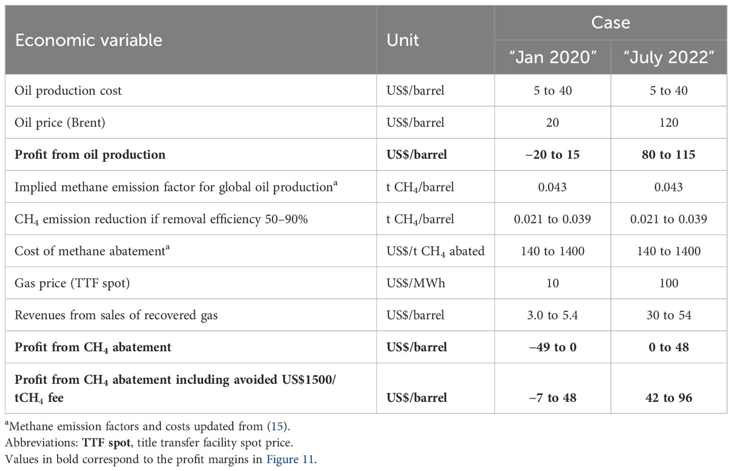
Table 3 Assumptions for the two fictive, illustrative cases “Jan 2020” and “July 2022”.
Figure 11
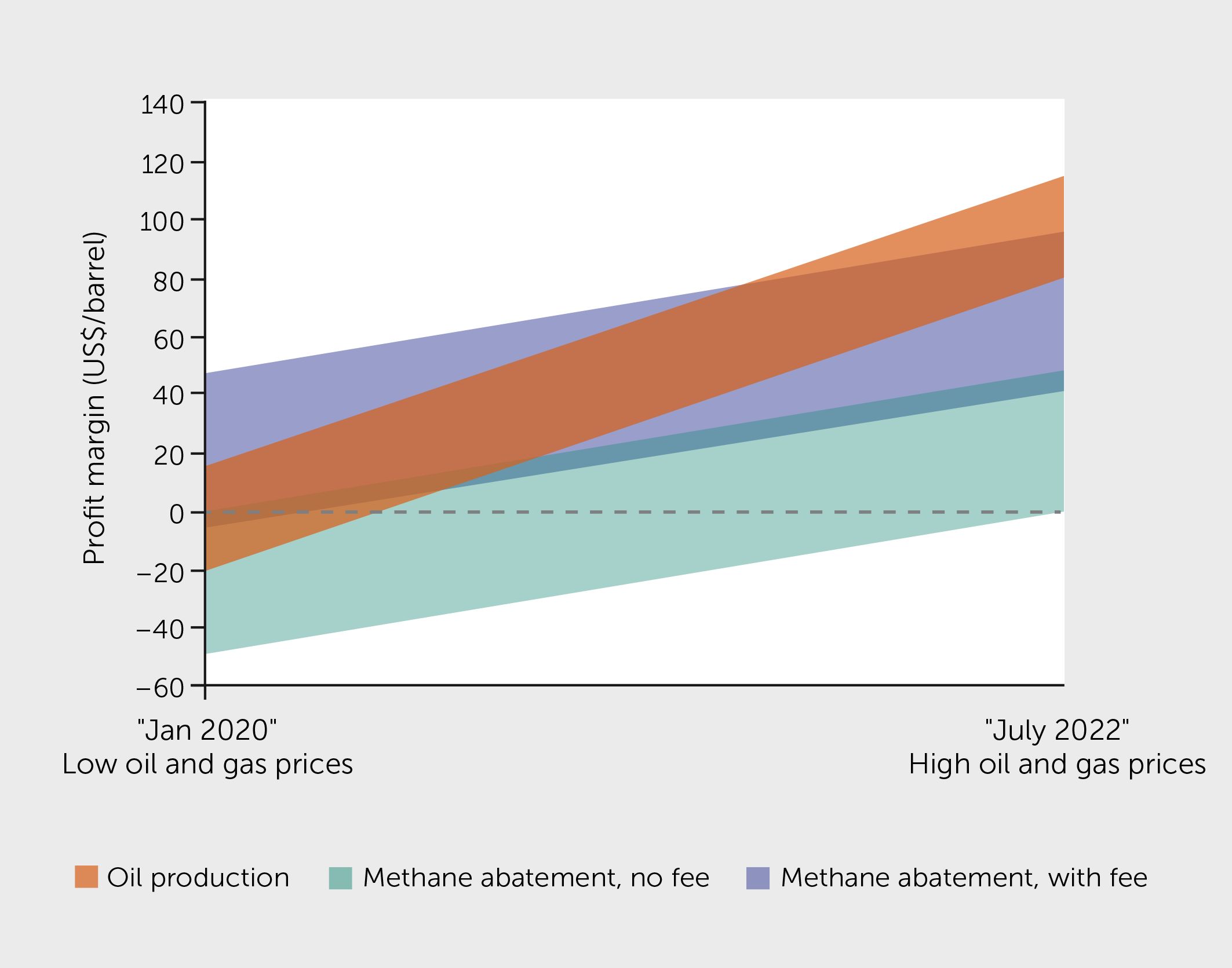
Figure 11 Variation in profit margins for oil production and methane abatement as fossil fuel prices change. Ranges for profit margins of oil production and methane abatement are shown for two illustrative cases “Jan 2020” and “July 2022” that correspond to historically low and high oil and gas prices, respectively (see Table 3 for assumptions). Profit margins for methane abatement are shown without a fee on emissions and with a US$1500 per tonne illustrative methane fee. See Methods (Analysis I) for further details.
This analysis helps explain the behavior of real-world markets, e.g., “Methane emissions remained stubbornly high in 2022 even as soaring energy prices made actions to reduce them cheaper than ever” (126). Profit-maximizing oil companies have a greater incentive to spend capital on increased production rather than voluntarily investing in methane control when prices are high, even though profits from such actions have increased. In such cases, oil companies can only be expected to invest in methane control if forced to do so through legally binding regulations. While actions to control methane from the fossil fuel sector entail substantial costs, the industry has ample resources compared with sectors such as waste or agriculture. For example, the IEA estimates that reducing energy-related methane emissions by 75% would require spending through 2030, which is <5% of the industry’s net 2023 income (127).
To reach abatement targets through private sector investments, policymakers need to ensure regulations are strong enough to overcome any competitive disadvantage of abatement investments relative to other operational investments. That measures are cost-effective from a societal perspective is no guarantee that abatement will happen without the introduction of additional regulations and policy incentives, such as requirements to use the best available technologies or a methane fee high enough to make abatement gains comparable to those available from new-source development from a private perspective (Figure 11). The imperatives to both reduce methane rapidly this decade and transition to net zero CO2 by the middle of the century imply that societies should consider granting companies social licenses to operate only if they are on course to both very low methane intensity by 2030 (including no routine venting or flaring) and to net zero CO2 by 2050.
Conclusions and next steps
The GMP has created enormous policy momentum. Alongside it, the Global Methane Hub (https://globalmethanehub.org/) links ~20 philanthropic organizations’ supporting action, and the CCAC links development banks with mitigation implementers. As such, there is an urgent need for expanded and improved knowledge of both the benefits of and opportunities for mitigation and access to finance to support the effective implementation of mitigation policies. This information can be provided with support tools that keep pace with rapidly advancing knowledge regarding current emission sources, especially via remote sensing.
Our analyses support three imperatives for methane mitigation. We illustrate how observations show increased methane concentration growth rates, which have recently reached the greatest values on record according to both ground-based and satellite data. Observed methane growth rates are now much higher than the mean predictions across models and far above levels consistent with Paris Climate Agreement goals. Human activities are predominantly responsible for the past ~15 years of growth—with contributions from increased emissions from wetlands due to anthropogenic global warming and from direct anthropogenic emissions. The first imperative is therefore to change course and reverse methane emission growth through stronger policy-led action targeting all major drivers of methane emissions as well as to greatly reduce CO2 emissions rapidly.
The second imperative is to align methane and CO2 mitigation. Major and rapid reductions in methane are integral to least-cost 1.5°C- and 2°C-consistent scenarios alongside the transformations needed to reach net zero CO2 by ~2050. However, net zero methane emissions is not the target owing to abatement challenges for some sources and its short lifetime. Nevertheless, since methane and CO2 each contribute to warming, maximizing reductions in methane emissions is important both for its own sake to ensure that 1.5°C- or 2°C-consistent CO2 trajectories are feasible and to reduce CDR requirements. Methane and CO2 mitigation actions are tightly interrelated: reducing methane emissions can directly contribute to reduced atmospheric CO2 via carbon cycle interactions. Focusing on land use, we quantify how decreased livestock numbers afforded by reduced consumption of cattle-based foods not only help reduce methane emissions but also free up land to help meet projected needs for CDR at levels required to achieve long-term climate goals. Rapid and deep cuts to CO2 and methane provide the strongest climate benefits across the century.
The third imperative highlights the need to optimize methane abatement policies. We show that both technological abatement options and systemic and behavioral choices must be addressed to reduce methane emissions. Our national-level analysis of methane mitigation opportunities highlights the need to address all subsectors when considering abatement options. We find that although many mitigation costs are low relative to real-world financial instruments and methane damage estimates, strong, legally binding regulations need to be in place even in the case of negative-cost options. To help policymakers and project funders, we created an online tool that explores different options and their cost-effectiveness. This tool supports policymakers by, for example, displaying (i) the most cost-effective options for countries to achieve a desired methane abatement objective economy-wide by sector or by subsector and (ii) the options in each country or countries that provide the largest abatement opportunities for a given spending level. Given substantial uncertainties in both emissions and costs, these data provide guidance for funders or policymakers who can then pursue more detailed studies. Funding equivalent to mitigation costs is not necessarily required since the cost analyses could support regulatory policies, e.g., by showing that they do not impose onerous burdens. For example, mitigation in the fossil sector is both large and low in cost in China and India, as are reductions in landfill methane in India, suggesting these two non-GMP countries have the potential to achieve major methane reductions with limited financial burdens.
The tool provides abatement potentials both as tonnes and percentages. The latter facilitates use with observations, for example, the identification of emission sources by satellites with global coverage but relatively low spatial resolution that are followed up by higher resolution site-specific quantification of emission rates (Figure 12). These data will soon be complemented by the satellite missions Carbon Mapper, MethaneSAT, GOSAT-GW, Sentinel-5, and Satlantis as well as datasets produced by the Integrated Global Greenhouse Gas Information System and the International Methane Emissions Observatory. Automated reporting based on satellite observations promises to provide rapid information on emissions and progress in abatement [e.g., (49), (107)] though updates to mitigation potentials and costs based on new data will take considerable time and effort.
Figure 12
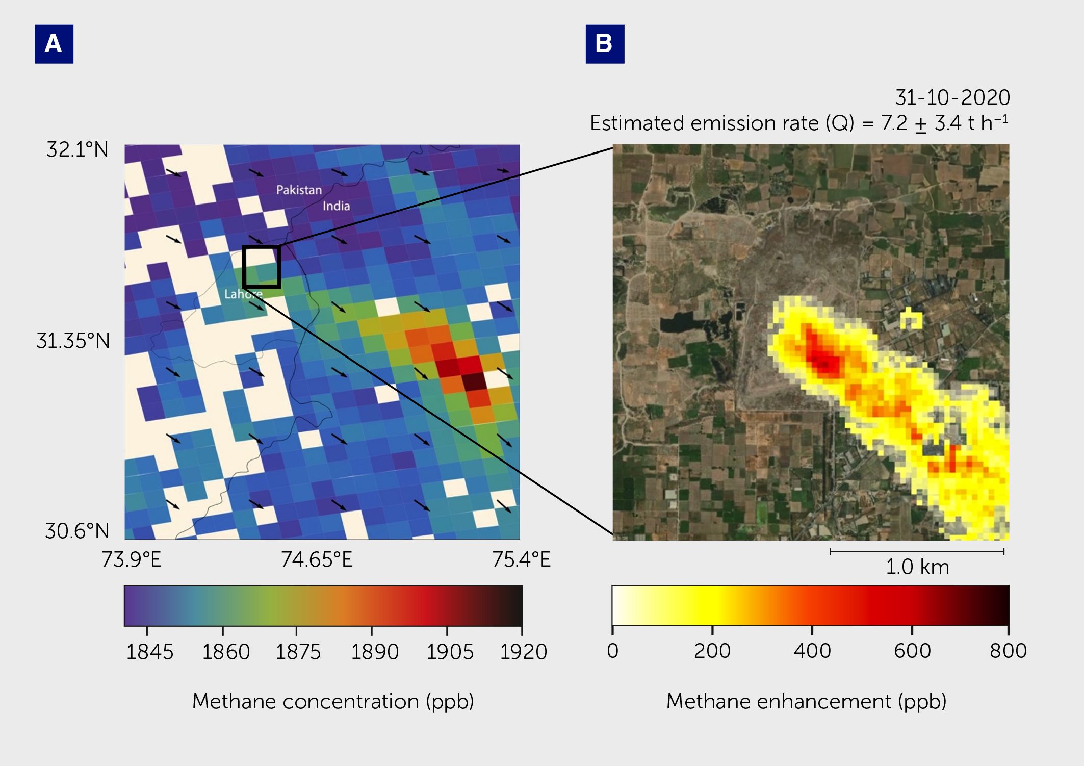
Figure 12 Example use of remote sensing to quantify methane emissions. (A) Methane observations from the TROPOMI instrument on 31 March 2019 over the region encompassing Lahore, Pakistan. (B) High-resolution measurement of methane enhancement over the northern part of the city observed by GHGSat on 31 October 2020. The emission source location matches the siting of the Lahore landfill, with Q indicating the estimated methane emission rate.
The new tool complements another showing the benefits of methane abatement (http://shindellgroup.rc.duke.edu/apps/methane/). That tool allows the user to select global or regional methane mitigation options by sector and cost and then displays national-level benefits including ozone effects on human health, yields for several major staple crops, heat-related labor productivity, and the economic valuation of these.
Though methane has similar environmental impacts wherever it is emitted, co-emissions affect those living near sources with environmental justice implications [e.g., (128, 129)]. These include hazardous hydrocarbons, such as benzene, that are frequently emitted by gas and oil facilities, black carbon from flaring, and ammonia from manure ponds. Methane-producing infrastructure is often in areas with high social vulnerability [e.g., (130)]. Accounting for co-emissions requires improved data on their spatial distribution and volume, especially in areas with nearby vulnerable populations.
There is also a need to improve understanding of several physical processes influencing the climate impacts of methane emissions. Methane-induced ozone increases affect the carbon cycle, amplifying the climate impact of methane, but the magnitude of this effect is highly uncertain (12). Additionally, methane affects particle formation via oxidants, producing aerosol-cloud interactions that may augment the climate impact of methane (131). Studies also report divergent results for the net cloud response to methane when the shortwave absorption of methane is accounted for (132, 133). A better understanding of the response of natural methane emissions to climate change is also needed. Improved capabilities to monitor emissions from difficult-to-access methane-source areas (e.g., wetlands) using remote sensing should help constrain changes in natural sources over the coming decade. A research agenda for methane removal technologies, which could be deployed in the unlikely event of a surge in natural emissions, has been called for [e.g., (134)] and is currently being assessed (https://www.nationalacademies.org/our-work/atmospheric-methane-removal-development-of-a-research-agenda).
Though additional observations and improved scientific understanding will be valuable, securing the benefits for climate, health, labor productivity, and crops (4, 79) that are the rationale for the GMP requires immediate implementation to achieve the emission reductions envisioned by 2030. Not only is our understanding of methane science and mitigation options sufficient to act upon, but political support is evidenced by the GMP, and financial support is growing. It is also becoming clearer how methane fees would achieve climate goals and enhance well-being. In the face of ever-increasing climate damages, including heat waves, flooding, storms, and fires, the world has a real opportunity to reduce the rate at which these effects grow between now and 2050 via methane action, with the main impediment being the will to implement the known solutions.
Methods
Analysis A: methane growth/emissions vs projections
Methane abundance growth rates during the 2020s are taken from “no climate policy” baseline scenarios from several recent multi-model intercomparison projects using integrated assessment models: ADVANCE (https://www.fp7-advance.eu/), NAVIGATE (https://www.navigate-h2020.eu/) (14), and ENGAGE (https://www.engage-climate.org/). NAVIGATE and ENGAGE scenarios are the most recent and include updates to actual trends in energy demand, costs, etc., and legislation through ~2020. This dataset includes results from the following IAMs: AIM/CGE 2.0, IMAGE (versions 3.0.1, 3.0.2, and 3.2), MESSAGE-GLOBIOM 1.0, MESSAGEix-GLOBIOM 1.1, POLES, REMIND 1.7, REMIND-MAgPIE (versions 1.5, 2.0–4.1, and 2.1–4.2), WITCH 5.0, and WITCH- GLOBIOM 4.2.
Baseline projections are also included from two “bottom-up” analyses by the International Institute for IIASA (15) and the EPA (16). The IIASA analysis uses their Greenhouse gas and Air pollution Interactions and Synergies (GAINS) model in which baseline emission estimates reflect expected impacts on emissions from current legislation to control emissions. Future methane emissions in GAINS by 2050 are developed based on macroeconomic and energy sector activity drivers from the IEA World Energy Outlook 2018 New Policies Scenario (135), agricultural sector activity drivers from the Food and Agricultural Organisation of the United Nations (FAO) (136), and IIASA’s own projections of solid waste and wastewater generation consistent with their relevant macroeconomic drivers. By incorporating policies projected forward by the IEA in 2018 in the energy scenario, these projections are expected to be similar to the NAVIGATE and ENGAGE baselines. The EPA’s projections are based on projected changes in underlying drivers taken from various globally available activity data sources depending on the source category. Trends in energy production and consumption are based on the United States Energy Information Administration 2017 International Energy Outlook Reference Case scenario. Growth rates in crop and livestock production are from International Food Policy Research Institute’s IMPACT model (International Model for Policy Analysis of Agricultural Commodities and Trade) (137). The full methodology is discussed in the documentation accompanying the EPA’s Global non-CO2 greenhouse gas emission projections & mitigation report (16). Neither the integrated assessment models nor the bottom-up analyses include changes in natural methane emissions.
A simple box model with a sink proportional to the atmospheric abundance of methane is used both to derive emission and sink estimates (Figure 1) and to convert scenario emissions to estimated concentration changes (Figure 2). The atmospheric residence time for methane is 9.1 years for 2020 methane concentrations in this model, consistent with the value reported in the IPCC AR6 (12).
Analysis B: projected methane emissions reductions under 1.5°C-consistent scenarios
This analysis utilizes the scenario dataset analyzed in the IPCC AR6 (59). We include all scenarios classified as being below 1.5°C in 2100 (>50% probability) with either no or limited overshoot and for which agricultural as well as total methane emissions were available. There are 53 scenarios from eight models that represent five separate model families: AIM/CGE 2.2 and AIM/Hub-Global 2.0; IMAGE 3.2; MESSAGE-GLOBIOM 1.1; REMIND 2.1, REMIND-MAgPIE 2.1–4.2 and 2.1–4.3; and WITCH 5.0. Data were obtained from the AR6 Scenario Database (86), release 1.1.
Analysis C: connection between land area use for BECCS and pasture
This analysis utilizes two sets of scenarios from the AR6 scenario database (86). We examine the relationship between the deployment of BECCS and the area used for pasture (area used for fodder was not available) using scenarios classified as keeping warming below 1.5°C with limited or no overshoot as well as those keeping warming below 1.5°C with high overshoot. The latter are included to obtain a larger sample of models given substantial intermodal variability in estimates of future BECCS deployment. Results are available from seven model families: AIM, GCAM, IMAGE, MESSAGE, REMIND, COFFEE, and WITCH. From these scenarios, we also analyze decadal changes in the multi-model means and individual scenarios for these two quantities from the 2040s (or 2030s) to 2090s.
A second set of scenarios is used to explore how land use trade-offs including land area used for afforestation vary across IAMs. We use an expanded set of scenarios classified as under 2°C as afforestation diagnostics were not available from as many models. Even using this larger dataset, we found only eight models that provided all the required outputs. As this analysis compares land used for carbon uptake (afforestation and bioenergy crops) with pasture area across multiple scenarios within a single model, we excluded three models that had six or fewer scenarios. One additional model, a variant of REMIND, has minimal changes in land deployed for carbon uptake so does not provide useful input for this analysis (though averages and ranges are not sensitive to the inclusion of that model). For the remaining four models (IMAGE 3.2, MESSAGEix-GLOBIOM 1.1, REMIND-MAgPIE 1.7–3.0, and WITCH 5.0), 22–106 scenarios were available (206 in total), allowing a robust characterization of the land use relationship for each of these models. In this analysis, afforestation is converted from the reported value in tCO2 to area using 12 tCO2 per ha (138).
Analysis D: climate impact of decarbonization and methane reduction
We analyzed the response of global mean annual average surface air temperatures to emissions under various scenarios to isolate the effects of decarbonization and targeted methane emission controls. The emissions scenarios are based upon the SSPs, using averages across 1.5°C scenarios (nominal 1.9 W m−2 forcing in 2100) under SSPs 1, 2, and 5 as 1.5°C was infeasible under SSP3 in four of four models and under SSP4 in two of three models. From those scenarios, we separate the effects of decarbonization from targeted methane abatement based on the methane abatement associated with decreasing fossil fuel use (4, 82, 95), which is classified as part of decarbonization, relative to all other methane reductions, which includes the remaining portion of fossil fuel-sector methane abatement and all methane abatement in the agriculture and waste sectors.
Temperature responses to those emissions relative to constant 2020 emissions were calculated using absolute global temperature potentials (AGTPs), as in prior work (4, 66, 78). The yearly AGTPs represent the global mean temperature change per kilogram of emission each year after those emissions based on an impulse-response function for the climate system, as is used in IPCC reports for selected example years, e.g., AGTP50 or AGTP100 (69). This analysis relies on AGTPs created using the transient climate response averaged over the last generation of climate models (CMIP5) (139), which is very similar to that reported from the latest generation (63). The response to methane is calibrated to match the global mean annual average temperature response from the full composition-climate models reported in the Global Methane Assessment’s climate simulations (4).
Analysis E: impact of methane abatement on temperature and health
This analysis presents global mean annual average temperature responses using the same methodology as Analysis D but in this case applied to scenarios based upon baseline and 1.5°C-consistent scenarios under the SSP2 pathway. SSP2 is chosen as it lies in the middle of the three for which models produced several 1.5°C consistent scenarios (SSPs 1, 2, and 5), consistent with its “middle-of-the-road” narrative description (96).
This analysis also presents health impacts based on changes in exposure to surface ozone. The GMA used five global composition-climate models to evaluate the effect of methane emissions on the maximum daily 8-hour ozone exposure averaged over the year (MDA8-annual). This was the metric most closely linked to increases in premature deaths from ozone in one of the largest epidemiological studies to date (140) as well as in a second large United States study that obtained very similar exposure-response results (141). This analysis utilizes the multi-model mean changes in this metric per unit methane emission change to derive the effect on human health due to reduced risk of both respiratory and cardiovascular premature mortality with decreasing ozone exposure.
We note that groups such as the EPA and Global Burden of Disease (GBD) do not include ozone-related cardiovascular premature deaths—the EPA’s expert panel reports that “evidence for long-term ozone exposure and cardiovascular effects is suggestive of, but insufficient to infer, a causal relationship” (142). However, a recent cohort study in China (143) reports a strong relationship and a much higher risk increment per unit exposure than that used here based on the United States studies. To characterize the range of potential methane-ozone-health impacts, we also evaluated the maximum daily 8-hour ozone exposure averaged over the 6-month period of maximum exposures (MDA8–6mon), the metric used in the Chinese epidemiological analysis. We apply the exposure–response relationship for cardiovascular disease of Niu et al. (143) using the same theoretical minimum risk exposure level (a threshold) as in the United States study [26.7 ppb (140)], as this value is below any exposures in Niu et al. The results are only modestly sensitive to the use of this threshold, however, with values ~20% less without the threshold, well within uncertainty ranges. We find 1930 [1110–2510: 95% confidence interval (CI)] deaths per Mt methane emission based on the exposure-response of Niu et al. (143), a best estimate value much larger than even the high end of the 690 (210–1120: 95% CI) deaths per MtCH4 found using the Turner et al. (140) relationship (4). Note that another large Chinese cohort study (144) reported more than double the increased risk of cardiovascular death due to increased ozone exposure relative to Niu et al. (143), suggesting that even our high-end estimate could be substantially too small.
In addition to the differing estimates of the effect of ozone on premature cardiovascular deaths, another recent analysis reports a strong relationship between ozone exposure and increased premature death in children aged under 5 years in low- and middle-income countries (145). Such an effect would be distinct from other effects analyzed here as the other studies included only populations aged 18 and older (143) or 30 and older (140). The impacts on children aged 0 to 5 were reported in response to MDA8–6mon, and we used this metric to again evaluate the effects of changing methane emissions for ozone exposures above 51 ppb, as reported in the epidemiological study. We find an additional 320 (125–485: 95% CI) premature deaths in children under 5.
Combining the 740 (460–990) adult respiratory deaths (4) with the adult cardiovascular deaths found here based on the Chinese cohort (143) and the under-5 age group deaths gives a total value of 3000 (2100–3600) per MtCH4. Using standard valuation methods (4), this leads to a valuation of US$5200 (3650–6250) per tCH4.
Human health impacts were calculated using 2015 population data from the Gridded Population of the World (GPW) version 4 (146) and 2015 baseline mortality rates from the GBD project (147) for each country of the world.
Analysis F: impact of methane abatement on heavy/outdoor labor
We assess the effects of changes in heat exposure due to mitigation of methane emissions on potential labor productivity within the heavy labor category, which primarily includes outdoor workers in agriculture, forestry and fisheries, and construction (100). The effects of methane abatement are evaluated relative to a “middle-of-the-road” SSP2 scenario, as in Analysis E. Uncertainties are characterized using multiple impact functions, namely those of Kjellstrom et al. (148), Foster et al. (149), and the International Organization for Standardization (ISO) Standard 7243 (150), using the approach of Bröde et al. (151). Analyses are performed for both the case of workers in the sun and in the shade.
Valuation of the avoided labor losses uses estimates from the International Labour Organization (ILO) of the fraction of the overall working-age population (ages 15–64) in each country that works in heavy labor (152), multiplied by the spatially gridded population ages 15–64 [Gridded Population of the World v4 data (146)] to estimate the number of workers in a given category and their spatial distribution. We then overlay the heavy labor hours lost by these workers to obtain total hours lost. We next calculate average value added per worker in agriculture, forestry and fisheries, and construction by dividing the total value added in 2017 (153) by the total working-age employment in a given category. This is then converted to value per hour assuming a 12-hour workday and 365 days/year (a maximalist assumption, though common in the labor economics literature, so the value of hours lost reported here is conservative). We then multiply the hourly value added per worker by the heavy labor hours lost to estimate the economic costs of heat-related productivity losses. Finally, values are converted from 2017 local currency units (LCU) to 2017 PPP-adjusted international dollars (2017 PPP$) by dividing a country’s LCU by its gross domestic product 2017 PPP conversion rate (LCU/US$). We sum the losses over all countries (n=163) to obtain the estimated global output loss.
Analysis G and H: national-level methane mitigation analysis of abatement potentials and costs
National mitigation potentials and their associated costs are evaluated primarily based on the data from the EPA (16) and from the IEA (90). The EPA data cover all sectors and include projected changes in both baseline emissions and mitigation. Mitigation potentials change over time due to factors such as projected technology turnover and improvements in technology over time. Potentials are estimated through 2050 and use a discount rate of 5% in cost estimates (e.g., for the value of captured gas). The IEA analysis includes only the fossil fuel sector and analyzes present-day abatement potentials associated with targeted control measures. This analysis uses a discount rate of 10% in its cost estimates.
Limited national data are also included from an analysis by IIASA, though this analysis is primarily done at the regional level (15). As with the EPA analysis, these mitigation potentials and costs cover all sectors and include time-dependent estimates of both changes in baseline emissions and mitigation. The latter include sector-specific assumptions about technology turnover times, based on the literature, improvements in technology over time, and the achievable pace of regulations. This analysis includes discount rates of 4% and 10% in their cost evaluation and also extends to 2050. EPA and IIASA data are evaluated for 2030 whereas IEA estimates are for 2022.
As presented in the main text, abatement options have been grouped into functionally similar categories to facilitate readability and allow comparison across estimates. An online tool facilitating analysis of the national level EPA and IEA has been created that allows users to sort the available national abatement options by sector according to their costs. The user can specify either a mitigation target or a spending target and can also compare across the EPA and IEA datasets (within the fossil fuel sector) and countries. The tool is available at https://github.com/psadavarte/Methane_mitigation_webtool.
Analysis I: profit/return from controlling methane emissions versus price (oil production)
To examine the implications of price fluctuations on oil companies’ incentives to invest in methane abatement, we compared two fictive cases called “Jan 2020” and “July 2022”. These approximate the situations in the global oil and gas markets in January 2020, when the world oil and gas prices stood at a historical low at ~US$20/barrel for oil (Brent) and about ~US$10/MWh for gas (title transfer facility [TTF] spot price), and July 2022, when the same prices stood at a historic high at about US$120/barrel for oil and US$100/MWh for gas. Our analysis assumes that there are no appreciable changes in the costs of oil production or methane abatement, the impact factors (methane released per barrel) for oil-related methane emissions, or the effectiveness of methane abatement to isolate the effects of commodity price changes.
Supplementary material
The Supplementary Material for this article can be found online at: https://www.frontiersin.org/articles/10.3389/fsci.2024.1349770/full#supplementary-material
Acknowledgments
We thank Katie Owens for analyses of AR6 scenarios and the Global Methane Hub for financial support.
Statements
Author contributions
DS: Conceptualization, Funding acquisition, Investigation, Supervision, Writing – original draft. PS: Investigation, Writing – review & editing. IA: Investigation, Visualization, Writing – review & editing. TB: Investigation, Writing – review & editing. GD: Writing – original draft. LH-I: Conceptualization, Investigation, Writing – original draft. BP: Investigation, Writing – review & editing. MS: Investigation, Writing – review & editing. GS: Investigation, Writing – review & editing. SS: Investigation, Writing – review & editing. KR: Data curation, Investigation, Visualization, Writing – review & editing. LP: Investigation, Writing – review & editing. ZQ: Writing – review & editing. GF: Writing – review & editing, Formal Analysis. JM: Investigation, Visualization, Writing – review & editing.
Data availability statement
The original contributions presented in the study are included in the article/Supplementary Material. Further inquiries can be directed to the corresponding author.
Funding
The author(s) declare financial support was received for the research, authorship, and/or publication of this article. This work was funded by the Global Methane Hub through Windward Fund Grant 016011-2022-01-01 and through the European Union FOCI program. The funders had no role in the study design; in the collection, analysis, and interpretation of data; in the writing of the report; and in the decision to submit the paper for publication.
Conflict of interest
The authors declare that the research was conducted in the absence of financial relationships that could be construed as a potential conflict of interest.
The reviewer FOC declared a past co-authorship with the author SS to the handling editor.
Publisher’s note
All claims expressed in this article are solely those of the authors and do not necessarily represent those of their affiliated organizations, or those of the publisher, the editors and the reviewers. Any product that may be evaluated in this article, or claim that may be made by its manufacturer, is not guaranteed or endorsed by the publisher.
References
1. Masson-Delmotte V, Zhai AP, Connors SL, Péan C, Berger S, Caud N, et al, editors. Climate Change 2021: The Physical Science Basis. Contribution of Working Group I to the Sixth Assessment Report of the Intergovernmental Panel on Climate Change. Cambridge: Cambridge University Press (2021). doi: 10.1017/9781009157896
2. Rosane P, Naran B, Ortega Pastor A, Conolly J, Wignarajah D. The landscape of methane abatement finance. Climate policy initiative (2022). Available at: https://www.climatepolicyinitiative.org/publication/the-landscape-of-methane-abatement-finance/.
3. Olczak M, Piebalgs A, Balcombe P. A global review of methane policies reveals that only 13% of emissions are covered with unclear effectiveness. One Earth (2023) 6(5):519–35. doi: 10.1016/j.oneear.2023.04.009
4. United Nations Environment Programme and Climate and Clean Air Coalition. Global Methane Assessment: Benefits and Costs of Mitigating Methane Emissions. Nairobi: UNEP (2021). Available at: https://www.unep.org/resources/report/global-methane-assessment-benefits-and-costs-mitigating-methane-emissions.
5. International Energy Agency. World Energy Outlook (2021) Paris: IEA. Available at: https://www.iea.org/reports/world-energy-outlook-2021/keeping-the-door-to-15–0c-open.
6. Shukla PR, Skea J, Slade R, Al Khourdajie R, van Diemen D, McCollum M, et al, editors. Climate Change 2022: Mitigation of Climate Change. Contribution of Working Group III to the Sixth Assessment Report of the Intergovernmental Panel on Climate Change. Cambridge: Cambridge University Press (2022). doi: 10.1017/9781009157926
7. Nisbet EG, Manning MR, Dlugokencky EJ, Fisher RE, Lowry D, Michel SE, et al. Very strong atmospheric methane growth in the 4 years 2014–2017: implications for the Paris Agreement. Global Biogeochem Cycles (2019) 33(3):318–42. doi: 10.1029/2018GB006009
8. Nisbet EG, Manning MR, Dlugokencky EJ, Michel SE, Lan X, Röckmann T, et al. Atmospheric methane: comparison between methane’s record in 2006–2022 and during glacial terminations. Global Biogeochem Cycles (2023) 37(8):e2023GB007875. doi: 10.1029/2023GB007875
9. Lan X, Thoning KW, Dlugokencky EJ. Trends in globally-averaged CH4, N2O, and SF6 determined from NOAA Global Monitoring Laboratory measurements. Version 2024–04. National Oceanic and Atmospheric Administration Global Monitoring Laboratory (2022). doi: 10.15138/P8XG-AA10.
10. World Meteorological Organization. WMO Greenhouse Gas Bulletin No. 19 – 15 November 2023. The State of Greenhouse Gases in the Atmosphere Based on Global Observations through 2022. Geneva: WMO (2023). Available at: https://library.wmo.int/idurl/4/68532.
11. Copernicus Atmospheric Monitoring Service. Greenhouse gas concentrations (2023). Available at: https://climate.copernicus.eu/climate-indicators/greenhouse-gas-concentrations.
12. Szopa S, Naik V, Adhikary B, Artaxo P, Berntsen T, Collins WD, et al. Short-lived climate forcers. In: Masson-Delmotte V, Zhai P, Pirani A, Connors SL, Péan C, Berger S, et al, editors. Climate Change 2021: the Physical Science Basis. Contribution of Working Group I to the Sixth Assessment Report of the Intergovernmental Panel on Climate Change. Cambridge: Cambridge University Press (2021) 817–922. doi: 10.1017/9781009157896.008
13. United Nations Environment Programme and Climate and Clean Air Coalition. Global Methane Assessment 2030 Baseline Report. Nairobi: UNEP (2022), Available at: https://www.unep.org/resources/report/global-methane-assessment-2030-baseline-report.
14. Harmsen M, Kriegler E, Van Vuuren DP, van der Wijst KI, Luderer G, Cui R, et al. Integrated assessment model diagnostics: key indicators and model evolution. Environ Res Lett (2021) 16(5):054046. doi: 10.1088/1748-9326/abf964
15. Höglund-Isaksson L, Gómez-Sanabria A, Klimont Z, Rafaj P, Schöpp W. Technical potentials and costs for reducing global anthropogenic methane emissions in the 2050 timeframe – results from the GAINS model. Environ Res Commun (2020) 2(2):025004, Available at: https://iopscience.iop.org/article/10.1088/2515-7620/ab7457. doi: 10.1088/2515-7620/ab7457
16. United States Environmental Protection Agency. Global Non-CO2 Greenhouse Gas Emission Projections & Mitigation [EPA-430-R-19-010]. Washington, DC: U.S. EPA (2019). Available at: https://www.epa.gov/sites/default/files/2019-09/documents/epa_non-co2_greenhouse_gases_rpt-epa430r19010.pdf.
17. Rogelj J, Shindell D, Jiang K, Fifita S, Forster P, Ginzburg V, et al. Mitigation pathways compatible with 1.5°C in the context of sustainable development. In: Masson-Delmotte V, Zhai P, Pörtner HO, Roberts D, Skea J, Shukla PR, et al, editors. Special Report on Global Warming of 1.5°C, Intergovernmental Panel on Climate Change. Cambridge: Cambridge University Press (2018) 93–174. doi: 10.1017/9781009157940.004
18. Jackson RB, Saunois M, Bousquet P, Canadell JG, Poulter B, Stavert AR, et al. Increasing anthropogenic methane emissions arise equally from agricultural and fossil fuel sources. Environ Res Lett (2020) 15(7):071002. doi: 10.1088/1748-9326/ab9ed2
19. Canadell JG, Monteiro PMS, Costa MH, Cotrim da Cunha L, Cox PM, Eliseev AV, et al. Global carbon and other biogeochemical cycles and feedbacks. In: Masson-Delmotte V, Zhai P, Pirani A, Connors SL, Péan C, Berger S, et al, editors. Climate Change 2021: The Physical Science Basis. Contribution of Working Group I to the Sixth Assessment Report of the Intergovernmental Panel on Climate Change. Cambridge: Cambridge University Press (2021) 673–816. doi: 10.1017/9781009157896.007
20. Zhang Z, Poulter B, Knox S, Stavert A, McNicol G, Fluet-Chouinard E, et al. Anthropogenic emission is the main contributor to the rise of atmospheric methane during 1993–2017. Natl Sci Rev (2022) 9(5):nwab200. doi: 10.1093/nsr/nwab200
21. Thanwerdas J, Saunois M, Berchet A, Pison I, Bousquet P. Investigation of the renewed methane growth post-2007 with high-resolution 3-D variational inverse modeling and isotopic constraints. Atmos Chem Phys (2024) 24(4):2129–67. doi: 10.5194/acp-24-2129-2024
22. Yin Y, Chevallier F, Ciais P, Bousquet P, Saunois M, Zheng B, et al. Accelerating methane growth rate from 2010 to 2017: leading contributions from the tropics and East Asia. Atmos Chem Phys (2021) 21(16):12631–47. doi: 10.5194/acp-21-12631-2021
23. Feng L, Palmer PI, Zhu S, Parker RJ, Liu Y. Tropical methane emissions explain large fraction of recent changes in global atmospheric methane growth rate. Nat Commun (2022) 13(1):1378. doi: 10.1038/s41467-022-28989-z
24. Oh Y, Zhuang Q, Welp LR, Liu L, Lan X, Basu S, et al. Improved global wetland carbon isotopic signatures support post-2006 microbial methane emission increase. Commun Earth Environ (2022) 3(1):1–12. doi: 10.1038/s43247-022-00488-5
25. Zhang Z, Poulter B, Feldman AF, Ying Q, Ciais P, Peng S, et al. Recent intensification of wetland methane feedback. Nat Clim Change (2023) 13(5):430–3. doi: 10.1038/s41558-023-01629-0
26. Gedney N, Huntingford C, Comyn-Platt E, Wiltshire A. Significant feedbacks of wetland methane release on climate change and the causes of their uncertainty. Environ Res Lett (2019) 14(8):84027. doi: 10.1088/1748-9326/ab2726
27. Thornhill G, Collins W, Olivié D, Skeie RB, Archibald A, Bauer S, et al. Climate-driven chemistry and aerosol feedbacks in CMIP6 Earth system models. Atmos Chem Phys (2021) 21(2):1105–26. doi: 10.5194/acp-21-1105-2021
28. Kleinen T, Gromov S, Steil B, Brovkin V. Atmospheric methane underestimated in future climate projections. Environ Res Lett (2021) 16(9):094006. doi: 10.1088/1748-9326/ac1814
29. Cheng CH, Redfern SAT. Impact of interannual and multidecadal trends on methane-climate feedbacks and sensitivity. Nat Commun (2022) 13(1):3592. doi: 10.1038/s41467-022-31345-w
30. Zhang Z, Zimmermann NE, Calle L, Hurtt G, Chatterjee A, Poulter B. Enhanced response of global wetland methane emissions to the 2015–2016 El Niño-Southern Oscillation event. Environ Res Lett (2018) 13(7):074009. doi: 10.1088/1748-9326/aac939
31. Froitzheim N, Majka J, Zastrozhnov D. Methane release from carbonate rock formations in the Siberian permafrost area during and after the 2020 heat wave. Proc Natl Acad Sci USA (2021) 118(32):e2107632118. doi: 10.1073/pnas.2107632118
32. Kleber GE, Hodson AJ, Magerl L, Mannerfelt ES, Bradbury HJ, Zhu Y, et al. Groundwater springs formed during glacial retreat are a large source of methane in the high Arctic. Nat Geosci (2023) 16(7):597–604. doi: 10.1038/s41561-023-01210-6
33. Chen Z, Balasus N, Lin H, Nesser H, Jacob DJ. African rice cultivation linked to rising methane. Nat Clim Change (2024) 14(2):148–51. doi: 10.1038/s41558-023-01907-x
34. Laughner JL, Neu JL, Schimel D, Wennberg PO, Barsanti K, Bowman KW, et al. Societal shifts due to COVID-19 reveal large-scale complexities and feedbacks between atmospheric chemistry and climate change. Proc Natl Acad Sci USA (2021) 118(46):e2109481118. doi: 10.1073/pnas.2109481118
35. Peng S, Lin X, Thompson RL, Xi Y, Liu G, Hauglustaine D, et al. Wetland emission and atmospheric sink changes explain methane growth in 2020. Nature (2022) 612(7940):477–82. doi: 10.1038/s41586-022-05447-w
36. Stevenson DS, Derwent RG, Wild O, Collins WJ. COVID-19 lockdown emission reductions have the potential to explain over half of the coincident increase in global atmospheric methane. Atmos Chem Phys (2022) 22(21):14243–52. doi: 10.5194/acp-22-14243-2022
37. Qu Z, Jacob DJ, Zhang Y, Shen L, Varon DJ, Lu X, et al. Attribution of the 2020 surge in atmospheric methane by inverse analysis of GOSAT observations. Environ Res Lett (2022) 17(9):094003. doi: 10.1088/1748-9326/ac8754
38. Feng L, Palmer PI, Parker RJ, Lunt MF, Bösch H. Methane emissions are predominantly responsible for record-breaking atmospheric methane growth rates in 2020 and 2021. Atmos Chem Phys (2023) 23(8):4863–80. doi: 10.5194/acp-23-4863-2023
39. Food and Agriculture Organization of the United Nations. FAOSTAT Online Statistical Service (2024). Available at: https://www.fao.org/statistics/en/.
40. CNBC. Mexico’s state oil company illegally flared more than US$342 million worth of hydrocarbons. CNBC (2023). Available at: https://www.cnbc.com/2023/01/18/Mexicos-pemex-illegally-flared-over-342-million-worth-of-hydrocarbons.html.
41. Lyon DR, Hmiel B, Gautam R, Omara M, Roberts KA, Barkley ZR, et al. Concurrent variation in oil and gas methane emissions and oil price during the COVID-19 pandemic. Atmos Chem Phys (2021) 21(9):6605–26. doi: 10.5194/acp-21-6605-2021
42. Plant G, Kort EA, Brandt AR, Chen Y, Fordice G, Gorchov Negron AM, et al. Inefficient and unlit natural gas flares both emit large quantities of methane. Science (2022) 377(6614):1566–71. doi: 10.1126/science.abq0385
43. Irakulis-Loitxate I, Guanter L, Maasakkers JD, Zavala-Araiza D, Aben I. Satellites detect abatable super-emissions in one of the world’s largest methane hotspot regions. Environ Sci Technol (2022) 56(4):2143–52. doi: 10.1021/acs.est.1c04873
44. Deng Z, Ciais P, Tzompa-Sosa ZA, Saunois M, Qiu C, Tan C, et al. Comparing national greenhouse gas budgets reported in UNFCCC inventories against atmospheric inversions. Earth Syst Sci Data (2022) 14(4):1639–75. doi: 10.5194/essd-14-1639-2022
45. Shen L, Gautam R, Omara M, Zavala-Araiza D, Maasakkers JD, Scarpelli TR, et al. Satellite quantification of oil and natural gas methane emissions in the US and Canada including contributions from individual basins. Atmos Chem Phys (2022) 22(17):11203–15. doi: 10.5194/acp-22-11203-2022
46. Sherwin ED, Rutherford JS, Zhang Z, Chen Y, Wetherley EB, Yakovlev PV, et al. US oil and gas system emissions from nearly one million aerial site measurements. Nature (2024) 627(8003):328–34. doi: 10.1038/s41586-024-07117-5
47. Duren RM, Thorpe AK, Foster KT, Rafiq T, Hopkins FM, Yadav V, et al. California’s methane super-emitters. Nature (2019) 575(7781):180–4. doi: 10.1038/s41586-019-1720-3
48. Lauvaux T, Giron C, Mazzolini M, d’Aspremont A, Duren R, Cusworth D, et al. Global assessment of oil and gas methane ultra-emitters. Science (2022) 375(6580):557–61. doi: 10.1126/science.abj4351
49. Schuit BJ, Maasakkers JD, Bijl P, Mahapatra G, Van den Berg A-W, Pandey S, et al. Automated detection and monitoring of methane super-emitters using satellite data. Atmos Chem Phys (2023) 23(16):9071–98. doi: 10.5194/acp-23-9071-2023
50. McNorton J, Bousserez N, Agustí-Panareda A, Balsamo G, Cantarello L, Engelen R, et al. Quantification of methane emissions from hotspots and during COVID-19 using a global atmospheric inversion. Atmos Chem Phys (2022) 22(9):5961–81. doi: 10.5194/acp-22-5961-2022
51. International Energy Agency. World Energy Investment 2022. Paris: IEA (2022). Available at: https://www.iea.org/reports/world-energy-investment-2022.
52. Oh Y, Bruhwiler L, Lan X, Basu S, Schuldt K, Thoning K, et al. CarbonTracker CH4 2023. National Oceanic and Atmospheric Administration Global Monitoring Laboratory (2023). doi: 10.25925/40JT-QD67
53. Hodson EL, Poulter B, Zimmermann NE, Prigent C, Kaplan JO. The El Niño–Southern Oscillation and wetland methane interannual variability. Geophys Res Lett (2011) 38(8):L08810. doi: 10.1029/2011GL046861
54. Zhu Q, Peng C, Ciais P, Jiang H, Liu J, Bousquet P, et al. Interannual variation in methane emissions from tropical wetlands triggered by repeated El Niño Southern Oscillation. Glob Change Biol (2017) 23(11):4706–16. doi: 10.1111/gcb.13726
55. Schaefer H, Smale D, Nichol SE, Bromley TM, Brailsford GW, Martin RJ, et al. Limited impact of el Niño–Southern Oscillation on variability and growth rate of atmospheric methane. Biogeosciences (2018) 15(21):6371–86. doi: 10.5194/bg-15-6371-2018
56. McNicol G, Fluet-Chouinard E, Ouyang Z, Knox S, Zhang Z, Aalto T, et al. Upscaling wetland methane emissions from the FLUXNET-CH4 eddy covariance network (UpCH4 v1. 0): model development, network assessment, and budget comparison. AGU Adv (2023) 4(5):e2023AV000956. doi: 10.1029/2023AV000956
57. Shaw JT, Allen G, Barker P, Pitt JR, Pasternak D, Bauguitte SJB, et al. Large methane emission fluxes observed from tropical wetlands in Zambia. Global Biogeochem Cycles (2022) 36(6):e2021GB007261. doi: 10.1029/2021GB007261
58. Pandey S, Houweling S, Lorente A, Borsdorff T, Tsivlidou M, Bloom AA, et al. Using satellite data to identify the methane emission controls of South Sudan’s wetlands. Biogeosciences (2021) 18(2):557–72. doi: 10.5194/bg-18-557-2021
59. Riahi K, Schaeffer R, Arango J, Calvin K, Guivarch C, Hasegawa T, et al. Mitigation pathways compatible with long-term goals. In: Shukla PR, Skea J, Slade R, Al Khourdajie R, van Diemen D, McCollum M, et al, editors. Climate Change 2022: Mitigation of Climate Change. Contribution of Working Group III to the Sixth Assessment Report of the Intergovernmental Panel on Climate Change. Cambridge: Cambridge University Press (2022) 295–408. doi: 10.1017/9781009157926.005
60. Allen MR, Peters GP, Shine KP, Azar C, Balcombe P, Boucher O, et al. Indicate separate contributions of long-lived and short-lived greenhouse gases in emission targets. npj Clim Atmos Sci (2022) 5:5. doi: 10.1038/s41612-021-00226-2
61. Arndt C, Hristov AN, Price WJ, McClelland SC, Pelaez AM, Cueva SF, et al. Full adoption of the most effective strategies to mitigate methane emissions by ruminants can help meet the 1.5°C target by 2030 but not 2050. Proc Natl Acad Sci USA (2022) 119(20):e2111294119. doi: 10.1073/pnas.2111294119
62. Ivanovich CC, Sun T, Gordon DR, Ocko IB. Future warming from global food consumption. Nat Clim Chang (2023) 13(3):297–302. doi: 10.1038/s41558-023-01605-8
63. Forster P, Storelvmo T, Armour K, Collins W, Dufresne J-L, Frame D, et al. The Earth’s energy budget, climate feedbacks, and climate sensitivity. In: Masson-Delmotte V, Zhai AP, Pirani A, Connors SL, Péan C, Berger S, et al, editors. Climate Change 2021: The Physical Science Basis. Contribution of Working Group I to the Sixth Assessment Report of the Intergovernmental Panel on Climate Change. Cambridge: Cambridge University Press (2021) 923–1054. doi: 10.1017/9781009157896.009
64. Collins WJ, Webber CP, Cox PM, Huntingford C, Lowe J, Sitch S, et al. Increased importance of methane reduction for a 1.5 degree target. Environ Res Lett (2018) 13(5):054003. doi: 10.1088/1748-9326/aab89c
65. Rogelj J, Lamboll RD. Substantial reductions in non-CO2 greenhouse gas emissions reductions implied by IPCC estimates of the remaining carbon budget. Commun Earth Environ (2024) 5:35. doi: 10.1038/s43247-023-01168-8
66. United Nations Environmental Programme. Emissions Gap Report. Nairobi: UNEP (2017). Available at: https://www.unep.org/resources/emissions-gap-report-2017.
67. Brazzola N, Wohland J, Patt A. Offsetting unabated agricultural emissions with CO2 removal to achieve ambitious climate targets. PloS One (2021) 16(3):e0247887. doi: 10.1371/journal.pone.0247887
68. Reisinger A, Geden O. Temporary overshoot: origins, prospects, and a long path ahead. One Earth (2023) 6(12):1631–7. doi: 10.1016/j.oneear.2023.11.008
69. Myhre G, Shindell D, Breon F-M, Collins W, Fuglestvedt J, Huang J, et al. Anthropogenic and Natural Radiative Forcing. In: Stocker TF, Qin D, Plattner GK, Tignor M, Allen SK, Boschung J, et al, editors. Climate Change 2013: The Physical Science Basis. Contribution of Working Group I to the Fifth Assessment Report of the Intergovernmental Panel on Climate Change. Cambridge: Cambridge University Press (2013) 659–740. Available at: https://www.cambridge.org/core/books/abs/climate-change-2013-the-physical-science-basis/anthropogenic-and-natural-radiative-forcing/63EB1057C36890FEAA4269F771336D4D.
70. Ocko IB, Hamburg SP, Jacob DJ, Keith DW, Keohane NO, Oppenheimer M, et al. Unmask temporal trade-offs in climate policy debates. Science (2017) 356(6337):492–3. doi: 10.1126/science.aaj2350
71. Shindell D, Borgford-Parnell N, Brauer M, Haines A, Kuylenstierna JCI, Leonard SA, et al. A climate policy pathway for near- and long-term benefits. Science (2017) 356(6337):493–4. doi: 10.1126/science.aak9521
72. Allen MR, Shine KP, Fuglestvedt JS, Millar RJ, Cain M, Frame DJ, et al. A solution to the misrepresentations of CO2-equivalent emissions of short- lived climate pollutants under ambitious mitigation. npj Clim Atmos Sci (2018) 1(1):16. doi: 10.1038/s41612-018-0026-8
73. Liu S, Proudman J, Mitloehner FM. Rethinking methane from animal agriculture. J Agric Biol Sci CABI (2021) 2(1):1–13. doi: 10.1186/s43170-021-00041-y
74. Ridoutt B. Climate neutral livestock production–A radiative forcing-based climate footprint approach. J Cleaner Prod (2021) 291:125260. doi: 10.1016/j.jclepro.2020.125260
75. Donnison CL, Murphy-Bokern D. Are climate neutrality claims in the livestock sector too good to be true? Environ Res Lett (2024) 19(1):011001. doi: 10.1088/1748-9326/ad0f75
76. Rogelj J, Schleussner C-F. Unintentional unfairness when applying new greenhouse gas emissions metrics at country level. Environ Res Lett (2019) 14(11):114039. doi: 10.1088/1748-9326/ab4928
77. West JJ, Fiore AM, Horowitz LW. Scenarios of methane emission reductions to 2030: abatement costs and co-benefits to ozone air quality and human mortality. Clim Change (2012) 114(3–4):441–61. doi: 10.1007/s10584-012-0426-4
78. Shindell DT, Fuglestvedt JS, Collins WJ. The social cost of methane: theory and applications. Faraday Discuss (2017) 200:429–51. doi: 10.1039/C7FD00009J
79. Mar KA, Unger C, Walderdorff L, Butler T. Beyond CO2 equivalence: the impacts of methane on climate, ecosystems, and health. Environ Sci Policy (2022) 134:127–36. doi: 10.1016/j.envsci.2022.03.027
80. Fu B, Gasser T, Li B, Tao S, Ciais P, Piao S, et al. Short-lived climate forcers have long-term climate impacts via the carbon–climate feedback. Nat Clim Change (2020) 10(9):851–5. doi: 10.1038/s41558-020-0841-x
81. Nzotungicimpaye CM, MacIsaac AJ, Zickfeld K. Delaying methane mitigation increases the risk of breaching the 2°C warming limit. Commun Earth Environ (2023) 4(1):250. doi: 10.1038/s43247-023-00898-z
82. Harmsen MJHM, van Vuuren DP, Bodirsky BL, Chateau J, Durand-Lasserve O, Drouet L, et al. The role of methane in future climate strategies: mitigation potentials and climate impacts. Clim Change (2019) 163(3):1409–25. doi: 10.1007/s10584-019-02437-2
83. Howarth RW, Jacobson MZ. How green is blue hydrogen? Energy Sci Eng (2021) 9(10):1676–87. doi: 10.1002/ese3.956
84. Ocko IB, Hamburg SP. Climate consequences of hydrogen emissions. Atmos Chem Phys (2022) 22(14):9349–68. doi: 10.5194/acp-22-9349-2022
85. Bertagni MB, Pacala SW, Paulot F, Porporato A. Risk of the hydrogen economy for atmospheric methane. Nat Commun (2022) 13(1):7706. doi: 10.1038/s41467-022-35419-7
86. Byers E, Krey V, Kriegler E, Riahi K, Schaeffer R, Jarmo K, et al. AR6 Scenarios Database hosted by International Institute for Applied Systems Analysis. (2022). Available at: doi: 10.5281/zenodo.5886911
87. Dooley K, Keith H, Larson A, Catacora-Vargas G, Carton W, Christiansen KL, et al. The Land Gap Report 2022. (2022). Available at: https://landgap.org/2022/report.
88. Hayek MN, Harwatt H, Ripple WJ, Mueller ND. The carbon opportunity cost of animal-sourced food production on land. Nat Sustain (2021) 4(1):21–4. doi: 10.1038/s41893-020-00603-4
89. Weber J, King JA, Abraham NL, Grosvenor DP, Smith CJ, Shin YM, et al. Chemistry-albedo feedbacks offset up to a third of forestation’s CO2 removal benefits. Science (2024) 383(6685):860–4. doi: 10.1126/science.adg6196
90. International Energy Agency. Global Methane Tracker 2023. Paris: IEA (2023). Available at: https://www.iea.org/reports/global-methane-tracker-2023.
91. Natural Resources Canada. Methane Centre of Excellence (2024). Available at: https://natural-resources.Canada.ca/climate-change/methane-centre-excellence/25656.
92. Andreae MO, Jones CD, Cox PM. Strong present-day aerosol cooling implies a hot future. Nature (2005) 435(7046):1187–90. doi: 10.1038/nature03671
93. Raes F, Seinfeld JH. New directions: climate change and air pollution abatement: a bumpy road. Atmos Environ (2009) 43(32):5132–3. doi: 10.1016/j.atmosenv.2009.06.001
94. Shindell D, Smith CJ. Climate and air-quality benefits of a realistic phase-out of fossil fuels. Nature (2019) 573(7774):408–11. doi: 10.1038/s41586-019-1554-z
95. Dreyfus GB, Xu Y, Shindell DT, Zaelke D, Ramanathan V. Mitigating Climate Disruption in Time: a self-consistent approach for avoiding both near-term and long-term global warming. Proc Natl Acad Sci USA (2022) 119(22):e2123536119. doi: 10.1073/pnas.2123536119
96. Riahi K, van Vuuren DP, Kriegler E, Edmonds J, O’Neill B, Fujimori S, et al. The Shared Socioeconomic Pathways and their energy, land use, and greenhouse gas emissions implications: an overview. Glob Environ Change (2017) 42:153–68. doi: 10.1016/j.gloenvcha.2016.05.009
97. Staniaszek Z, Griffiths PT, Folberth GA, O’Connor FM, Abraham NL, Archibald AT. The role of future anthropogenic methane emissions in air quality and climate. npj Clim Atmos Sci (2022) 5(1):1–8. doi: 10.1038/s41612-022-00247-5
98. Jones CD, Frölicher TL, Koven C, MacDougall AH, Matthews HD, Zickfeld K, et al. The Zero Emissions Commitment Model Intercomparison Project (ZECMIP) contribution to C4MIP: quantifying committed climate changes following zero carbon emissions. Geosci Model Dev (2019) 12(10):4375–85. doi: 10.5194/gmd-12-4375-2019
99. Palazzo Corner S, Siegert M, Ceppi P, Fox-Kemper B, Frölicher TL, Gallego-Sala A, et al. The Zero Emissions Commitment and climate stabilization. Front Sci (2023) 1:1170744. doi: 10.3389/fsci.2023.1170744
100. Parsons LA, Shindell D, Tigchelaar M, Zhang Y, Spector JT. Increased labor losses and decreased adaptation potential in a warmer world. Nat Commun (2021) 12:7286. doi: 10.1038/s41467-021-27328-y
101. Saunois M, Stavert AR, Poulter B, Bousquet P, Canadell JG, Jackson RB, et al. The global methane budget 2000–2017. Earth Syst Sci Data (2020) 12(3):1561–623. doi: 10.5194/essd-12-1561-2020
102. Nisbet EG, Fisher RE, Lowry D, France JL, Allen G, Bakkaloglu S, et al. Methane mitigation: methods to reduce emissions, on the path to the Paris agreement. Rev Geophys (2020) 58(1):RG000675:e2019. doi: 10.1029/2019RG000675
103. Willett W, Rockström J, Loken B, Springmann M, Lang T, Vermeulen S, et al. Food in the Anthropocene: the EAT–Lancet Commission on healthy diets from sustainable food systems. Lancet (2019) 393(10170):447–92. doi: 10.1016/S0140-6736(18)31788-4
104. Babiker M, Berndes G, Blok K, Cohen B, Cowie A, Geden O, et al. Cross-sectoral perspectives. In: Shukla PR, Skea J, Slade R, Al Khourdajie R, van Diemen D, McCollum M, et al, editors. Climate Change 2022: Mitigation of Climate Change. Contribution of Working Group III to the Sixth Assessment Report of the Intergovernmental Panel on Climate Change. Cambridge: Cambridge University Press (2022) 1245–1354 . Available at: https://www.ipcc.ch/report/ar6/wg3/.
105. Harrison MT, Cullen BR, Mayberry DE, Cowie AL, Bilotto F, Badgery WB, et al. Carbon myopia: the urgent need for integrated social, economic and environmental action in the livestock sector. Glob Change Biol (2021) 27(22):5726–61. doi: 10.1111/gcb.15816
106. Global Methane Hub and ClimateWorks Foundation. Global Innovation Needs Assessments: Food System Methane [Technical Report]. ClimateWorks Foundation (2023). Available at: https://www.climateworks.org/ginas-methane/.
107. Wang Y, Guo X, Huo Y, Li M, Pan Y, Yu S, et al. Toward a versatile spaceborne architecture for immediate monitoring of the global methane pledge. Atmos Chem Phys (2023) 23(9):5233–49. doi: 10.5194/acp-23-5233-2023
108. Pandey S, Gautam R, Houweling S, van der Gon HD, Sadavarte P, Borsdorff T, et al. Satellite observations reveal extreme methane leakage from a natural gas well blowout. Proc Natl Acad Sci USA (2019) 116(52):26376–81. doi: 10.1073/pnas.1908712116
109. Varon DJ, Jacob DJ, Jervis D, McKeever J. Quantifying time-averaged methane emissions from individual coal mine vents with GHGSat-D satellite observations. Environ Sci Technol (2020) 54(16):10246–53. doi: 10.1021/acs.est.0c01213
110. Sadavarte P, Pandey S, Maasakkers JD, Lorente A, Borsdorff T, Denier van der Gon H, et al. Methane emissions from superemitting coal mines in Australia quantified using TROPOMI satellite observations. Environ Sci Technol (2021) 55(24):16573–80. doi: 10.1021/acs.est.1c03976
111. de Foy B, Schauer JJ, Lorente A, Borsdorff T. Investigating high methane emissions from urban areas detected by TROPOMI and their association with untreated wastewater. Environ Res Lett (2023) 18(4):044004. doi: 10.1088/1748-9326/acc118
112. Maasakkers JD, Varon DJ, Elfarsdóttir A, McKeever J, Jervis D, Mahapatra G, et al. Using satellites to uncover large methane emissions from landfills. Sci Adv (2022) 8(31):eabn9683. doi: 10.1126/sciadv.abn9683
113. Chen Z, Jacob DJ, Nesser H, Sulprizio MP, Lorente A, Varon DJ, et al. Methane emissions from China: a high-resolution inversion of TROPOMI satellite observations. Atmos Chem Phys (2022) 22(16):10809–26. doi: 10.5194/acp-22-10809-2022
114. United States Environmental Protection Agency. Report on the Social Cost of Greenhouse Gases: Estimates Incorporating Recent Scientific Advances. Washington, DC: U.S. EPA (2023). Available at: https://www.epa.gov/environmental-economics/scghg.
115. Climate Impact Lab. Data-Driven Spatial Climate Impact Model User Manual. [Version 092022-EPA]. Climate Impact Lab (2022). Available at: https://impactlab.org/research/dscim-user-manual-version-092022-epa.
116. Rennert K, Errickson F, Prest BC, Rennels L, Newell RG, Pizer W, et al. Comprehensive evidence implies a higher social cost of CO2. Nature (2022) 610(7933):687–92. doi: 10.1038/s41586-022-05224-9
117. Howard PH, Sterner T. Few and not so far between: a meta-analysis of climate damage estimates. Environ Resour Econ (2017) 68(1):197–225. doi: 10.1007/s10640-017-0166-z
118. Wang T, Teng F. Damage function uncertainty increases the social cost of methane and nitrous oxide. Nat Clim Change (2023) 13(11):–1258–65. doi: 10.1038/s41558-023-01803-4
119. Melvin AM, Sarofim MC, Crimmins AR. Climate benefits of U.S. EPA programs and policies that reduced methane emissions 1993–2013. Environ Sci Technol (2016) 50(13):6873–81. doi: 10.1021/acs.est.6b00367
120. Sarofim MC, Waldhoff ST, Anenberg SC. Valuing the ozone-related health benefits of methane emission controls. Environ Resour Econ (2017) 66(1):45–63. doi: 10.1007/s10640-015-9937-6
121. Vandyck T, Keramidas K, Tchung-Ming S, Weitzel M, Van Dingenen R. Quantifying air quality co-benefits of climate policy across sectors and regions. Clim Change (2020) 163(3):1501–17. doi: 10.1007/s10584-020-02685-7
122. Sampedro J, Waldhoff S, Sarofim M, Van Dingenen R. Marginal damage of methane emissions: ozone impacts on agriculture. Environ Resour Econ (2023) 84(4):1095–126. doi: 10.1007/s10640-022-00750-6
123. California Air Resources Board. Cap-and-Trade Program (2023). Available at: https://ww2.arb.ca.gov/our-work/programs/cap-and-trade-program.
124. Parry I, Black S, Minnett D, Mylonas V, Vernon N. How to cut methane emissions. IMF Staff Climate Note 2022/008. Washington, DC: International Monetary Fund (2022).
125. Nordhaus W. Projections and uncertainties about climate change in an era of minimal climate policies. Am Econ J Econ Policy (2018) 10(3):333–60. doi: 10.1257/pol.20170046
126. International Energy Agency. Methane emissions remained stubbornly high in 2022 even as soaring energy prices made actions to reduce them cheaper than ever (2023). Available at: https://www.iea.org/news/methane-emissions-remained-stubbornly-high-in-2022-even-as-soaring-energy-prices-made-actions-to-reduce-them-cheaper-than-ever.
127. International Energy Agency. Global Methane Tracker 2024. Paris: IEA (2024). Available at: https://www.iea.org/reports/global-methane-tracker-2024.
128. Buonocore J, Reka S, Yang D, Chang C, Roy A, Thompson T, et al. Air pollution and health impacts of oil & gas production in the United States. Env Res Health (2023) 1(2):021006. doi: 10.1088/2752-5309/acc886
129. Chen C, McCabe DC, Fleischman LE, Cohan DS. Black carbon emissions and associated health impacts of gas flaring in the United States. Atmosphere (2022) 13(3):385. doi: 10.3390/atmos13030385
130. Emanuel RE, Caretta MA, Rivers IIIL, Vasudevan P. Natural gas gathering and transmission pipelines and social vulnerability in the United States. GeoHealth (2021) 5(6):e2021GH000442. doi: 10.1029/2021GH000442
131. O’Connor FM, Johnson BT, Jamil O, Andrews T, Mulcahy JP, Manners J. Apportionment of the pre-industrial to present-day climate forcing by methane using UKESM1: the role of the cloud radiative effect. J Adv Model Earth Syst (2022) 14(10):e2022MS002991. doi: 10.1029/2022MS002991
132. Smith CJ, Kramer RJ, Myhre G, Forster PM, Soden BJ, Andrews T, et al. Understanding rapid adjustments to diverse forcing agents. Geophys Res Lett (2018) 45(21):12–023. doi: 10.1029/2018GL079826
133. Allen RJ, Zhao X, Randles CA, Kramer RJ, Samset BH, Smith CJ. Surface warming and wetting due to methane’s long-wave radiative effects muted by short-wave absorption. Nat Geosci (2023) 16(4):314–20. doi: 10.1038/s41561-023-01144-z
134. Jackson RB, Abernethy S, Canadell JG, Cargnello M, Davis SJ, Féron S, et al. Atmospheric methane removal: a research agenda. Philos Trans A Math Phys Eng Sci (2021) 379(2210):20200454. doi: 10.1098/rsta.2020.0454
135. International Energy Agency. World Energy Outlook 2018. Paris: IEA (2018). Available at: https://www.iea.org/reports/world-energy-outlook-2018.
136. Alexandratos N, Bruisma J. World Agriculture Towards 2030/2050–The 2012 Revision, ESA Working Paper No. 12–03. Rome: Agricultural Development Economics Unit, Food and Agricultural Organization of the United Nations (2012). Available at: https://www.fao.org/4/ap106e/ap106e.pdf.
137. Robinson S, Mason d’Croz D, Islam S, Sulser TB, Robertson RD, Zhu T, et al. The International Model for Policy Analysis of Agricultural Commodities and Trade (Impact): model description for version 3 [IFRI discussion paper 1483]. Washington, DC: International Food Policy Research Institute (2015). Available at: https://www.ifpri.org/publication/international-model-policy-analysis-agricultural-commodities-and-trade-impact-model-0.
138. Bernal B, Murray LT, Pearson TRH. Global carbon dioxide removal rates from forest landscape restoration activities. Carbon Balance Manag (2018) 13(1):22. doi: 10.1186/s13021-018-0110-8
139. Geoffroy O, Saint-Martin D, Bellon G, Voldoire A, Olivié DJL, Tytéca S. Transient climate response in a two-layer energy-balance model. Part II: Representation of the efficacy of deep-ocean heat uptake and validation for CMIP5 AOGCMs. J Climate (2013) 26(6):1859–76. doi: 10.1175/JCLI-D-12-00196.1
140. Turner MC, Jerrett M, Pope CA, Krewski D, Gapstur SM, Diver WR, et al. Long-term ozone exposure and mortality in a large prospective study. Am J Respir Crit Care Med (2016) 193(10):1134–42. doi: 10.1164/rccm.201508-1633OC
141. Lim CC, Hayes RB, Ahn J, Shao Y, Silverman DT, Jones RR, et al. Long-term exposure to ozone and cause-specific mortality risk in the United States. Am J Respir Crit Care Med (2019) 200(8):1022–31. doi: 10.1164/rccm.201806-1161OC
142. United States Environmental Protection Agency. Integrated Science Assessment (ISA) for Ozone and Related Photochemical Oxidants (Final report, Apr 2020). Washington, DC: U.S. EPA (2020). Available at: https://cfpub.epa.gov/ncea/isa/recordisplay.cfm?deid=348522.
143. Niu Y, Zhou Y, Chen R, Yin P, Meng X, Wang W, et al. Long-term exposure to ozone and cardiovascular mortality in China: a nationwide cohort study. Lancet Planet Health (2022) 6(6):e496–503. doi: 10.1016/S2542-5196(22)00093-6
144. Liu S, Zhang Y, Ma R, Liu X, Liang J, Lin H, et al. Long-term exposure to ozone and cardiovascular mortality in a large Chinese cohort. Environ Int (2022) 165:107280. doi: 10.1016/j.envint.2022.107280
145. Xue T, Wang R, Tong M, Kelly FJ, Liu H, Li J, et al. Estimating the exposure–response function between long-term ozone exposure and under-5 mortality in 55 low-income and middle-income countries: a retrospective, multicentre, epidemiological study. Lancet Planet Health (2023) 7(9):e736–46. doi: 10.1016/S2542-5196(23)00165-1
146. Center for International Earth Science Information Network, Columbia University, Food and Agriculture Programme of the United Nations, and Centro Internacional de Agricultura Tropical. Gridded Population of the World, Version 4 (GPWv4): Population Count Grid. Palisades, NY: National Aeronautics and Space Administration Socioeconomic Data and Applications Center (2016). Available at: https://sedac.ciesin.columbia.edu/data/collection/gpw-v4.
147. Global Burden of Disease Collaborative Network. Global Burden of Disease Study 2017 (GBD 2017). Seattle, WA: The Institute for Health Metrics and Evaluation (2017).
148. Kjellstrom T, Freyberg C, Lemke B, Otto M, Briggs D. Estimating population heat exposure and impacts on working people in conjunction with climate change. Int J Biometeorol (2018) 62(3):291–306. doi: 10.1007/s00484-017-1407-0
149. Foster J, Smallcombe JW, Hodder S, Jay O, Flouris AD, Nybo L, et al. An advanced empirical model for quantifying the impact of heat and climate change on human physical work capacity. Int J Biometeorol (2021) 65(7):1215–29. doi: 10.1007/s00484-021-02105-0
150. International Organization for Standardization. Ergonomics of the Thermal Environment — Assessment of Heat Stress Using the WBGT (Wet Bulb Globe Temperature) index [ISO Standard 7243:2017]. Geneva: ISO (2017). Available at: https://www.iso.org/standard/67188.html.
151. Bröde P, Fiala D, Lemke B, Kjellstrom T. Estimated work ability in warm outdoor environments depends on the chosen heat stress assessment metric. Int J Biometeorol (2018) 62(3):331–45. doi: 10.1007/s00484-017-1346-9
152. International Labour Organization. Employment by sex and age — ILO modelled estimates. ILOSTAT Database (2023). Available at: https://ilostat.ilo.org/data.
153. World Bank. World Bank Open Data (2021). Available at: https://data.worldbank.org/.
Keywords: methane emissions, climate change mitigation, ozone, CO2 budget, mitigation costs, fossil fuels, net zero, livestock
Citation: Shindell D, Sadavarte P, Aben I, Bredariol TdO, Dreyfus G, Höglund-Isaksson L, Poulter B, Saunois M, Schmidt GA, Szopa S, Rentz K, Parsons L, Qu Z, Faluvegi G and Maasakkers JD. The methane imperative. Front Sci (2024) 2:1349770. doi: 10.3389/fsci.2024.1349770
Received: 05 December 2023; Accepted: 06 June 2024;
Published: 30 July 2024.
Edited by:
Euan Nisbet, Royal Holloway University of London, United KingdomReviewed by:
Fiona O’Connor, Met Office Hadley Centre (MOHC), United KingdomAndy Reisinger, Australian National University, Australia
Copyright © 2024 Shindell, Sadavarte, Aben, Bredariol, Dreyfus, Höglund-Isaksson, Poulter, Saunois, Schmidt, Szopa, Rentz, Parsons, Qu, Faluvegi and Maasakkers. This is an open-access article distributed under the terms of the Creative Commons Attribution License (CC BY). The use, distribution or reproduction in other forums is permitted, provided the original author(s) and the copyright owner(s) are credited and that the original publication in this journal is cited, in accordance with accepted academic practice. No use, distribution or reproduction is permitted which does not comply with these terms.
*Correspondence: Drew Shindell, ZHJldy5zaGluZGVsbEBkdWtlLmVkdQ==