 Chris Henry†
- Department of Earth Sciences, Simon Fraser University, Burnaby, BC, Canada
Groundwater recharge in southern Mali is investigated using interpretive recharge models and stable isotopes to identify the dominant recharge mechanism and explore how local variations in geological materials influence the recharge characteristics. At a regional scale, the groundwater level hydrographs from across southern Mali (1998–2002) are relatively consistent, showing seasonal variations, suggesting diffuse recharge is the dominant mechanism. Groundwater samples plot within the range of the weighted mean monthly δ18O and δ2H concentrations for July-August-September rainfall, and below the weighted mean annual δ18O and δ2H concentrations for rainfall, suggesting a dominantly rainy season source of recharge. Recharge is simulated for four representative unsaturated zone environments, each with varying soil, laterite and sedimentary bedrock layers, and three ranges of water table depths, for a total of 12 combinations. The simulated recharge response starts in July, 1 month after the arrival of the rainy season, and recharge is greatly accelerated through August to its peak in September. On an annual basis, ~72% of annual rainfall occurs between July and September, and nearly 60% of simulated recharge occurs between August and October. The simulated regional average annual recharge is 519 mm/year (479–560 mm/year range among models). By comparison, recharge estimated from the observed storage anomaly hydrographs using the water table fluctuation method is 384 mm/year (189–619 mm/year) using a specific yield of 0.05, although the range could be as high as 83–772 mm/year given the uncertainty in specific yield values (0.02–0.07). The simulated recharge also agrees with the timing of regional observed storage anomalies for all observation wells, but somewhat less so for the regional GRACE storage anomaly (2002–2008), which has a slower rate of rise in storage and a faster rate of recession compared to the observed storage anomalies and simulated recharge response.
Introduction
Long-term average groundwater recharge is the major limiting factor for the sustainable use of groundwater (Döll and Fiedler, 2008). Yet estimating recharge is very challenging because it cannot be measured directly (Healy, 2010), nor is there a widely applicable method for directly and accurately quantifying how much precipitation reaches the water table (Scanlon et al., 2002a; Healy, 2010). For this reason, studies often employ combinations of methods for estimating recharge, spanning numerical models at different spatial (global through local) and temporal (daily to multi-decadal) scales and in dimension (one-, two-, and three-dimensional), methods based on remote sensing data such as the Gravity Recovery And Climate Experiment (GRACE), and a wide range of field-based methods including the water table fluctuation (WTF) method, water balance methods, the chloride mass balance (CMB) method, methods employing environmental isotopes and tracers (including heat), methods based on surface water data, among others (Scanlon et al., 2002a; Healy, 2010). To guide the selection of recharge estimation method, it is important to develop a conceptual model of recharge processes, so that the most appropriate estimation techniques are used (Healy, 2010). Equally, it is important to consider the spatial scale of the estimation method. Global scale models, for example, have been shown to underestimate large decadal declining and rising water storage trends relative to GRACE data (Scanlon et al., 2018), and point estimates of recharge using the CMB method, for example, may not be easily reconciled with regional scale estimates (Pavlovskii et al., 2019). It is also important to consider the temporal scale of the estimation method. For example, in arid (and semi-arid) areas where annual precipitation is less than annual evapotranspiration, using a yearly or monthly time scale in a water balance can lead to an underestimation of the recharge (Chung et al., 2016).
Complicating the estimation of recharge is that there may be different recharge mechanisms, and many recharge estimation methods cannot distinguish which process dominates (MacDonald et al., 2021). While diffuse recharge tends to dominate in humid climates, and focused recharge tends to dominate in arid and semi-arid climates (Scanlon et al., 2006), recharge to a groundwater system can occur via both mechanisms in different areas or in the same area but at different times of the year, depending on climate (e.g., Meixner et al., 2016). Diffuse recharge is distributed across the landscape and results from precipitation infiltrating through the unsaturated zone to the saturated zone across a large area. Diffuse recharge is spatially variable and typically varies seasonally. Focused recharge is more localized and results from losses generated during episodic rain events from ephemeral streamflow or from water-filled topographic depressions in the land surface. Recent research has highlighted the complexity and episodic nature of focused recharge, and its large year-to-year variability (Taylor et al., 2013). In the case of depression-focused recharge, each depression may only occupy a small area (e.g., <100 m2), but collectively they can cover a sizable fraction (e.g., a few percent) of the landscape. Therefore, in regions with a high density of small depressions, depression-focused recharge can be the dominant recharge mechanism (e.g., Pavlovskii et al., 2019).
Chung et al. (2016) explored the main advantages and disadvantages of different recharge estimation methods used in semi-arid and humid regions of Africa. While they determined that the WTF, Recession-Curve Displacement, and CMB methods are perhaps the most reliable methods, they suggested that due to lack of basic data, remote sensing and watershed hydrological modeling should be used. However, field measurements are essential for ground-truthing remote sensing data and for calibrating hydrological models. In recent years, significant advancements have been made on estimating recharge in Africa using observational data. MacDonald et al. (2021) mapped the long-term (multi-decadal) average distributed groundwater recharge rates across Africa for the period 1970–2019 from 134 ground-based estimates. While that study represents a tremendous effort to integrate and interpret ground-based data, the distribution of data points (Figure 1 in MacDonald et al., 2021) remains relatively sparse, particularly given the wide range of climate zones across the African continent.
Cuthbert et al. (2019) used groundwater level hydrographs collated from across the African continent to explore the relationships between precipitation and recharge across a diverse range of climatic and geological contexts. They found that the transition from focused-dominated to diffuse-dominated recharge occurs around the boundary between semi-arid and sub-humid conditions, and that levels of aridity (i.e., the ratio of long-term precipitation to potential evapotranspiration, P/PET) dictates the predominant recharge processes, whereas local hydrogeology influences the type and sensitivity of precipitation–recharge relationships (Figure 4 in Cuthbert et al., 2019).
This study focuses on southern Mali. With a climate transitioning from semi-arid near Bamako to mid-humid, sub-tropical to the south near Bougouni (Figure 1), the dominant recharge mechanism could be either focused (episodic events) or diffuse (seasonal). Therefore, the purpose of the study is to explore the characteristics of recharge in southern Mali with the aim of identifying the dominant recharge mechanism and how local variations in geological materials influence the recharge characteristics.
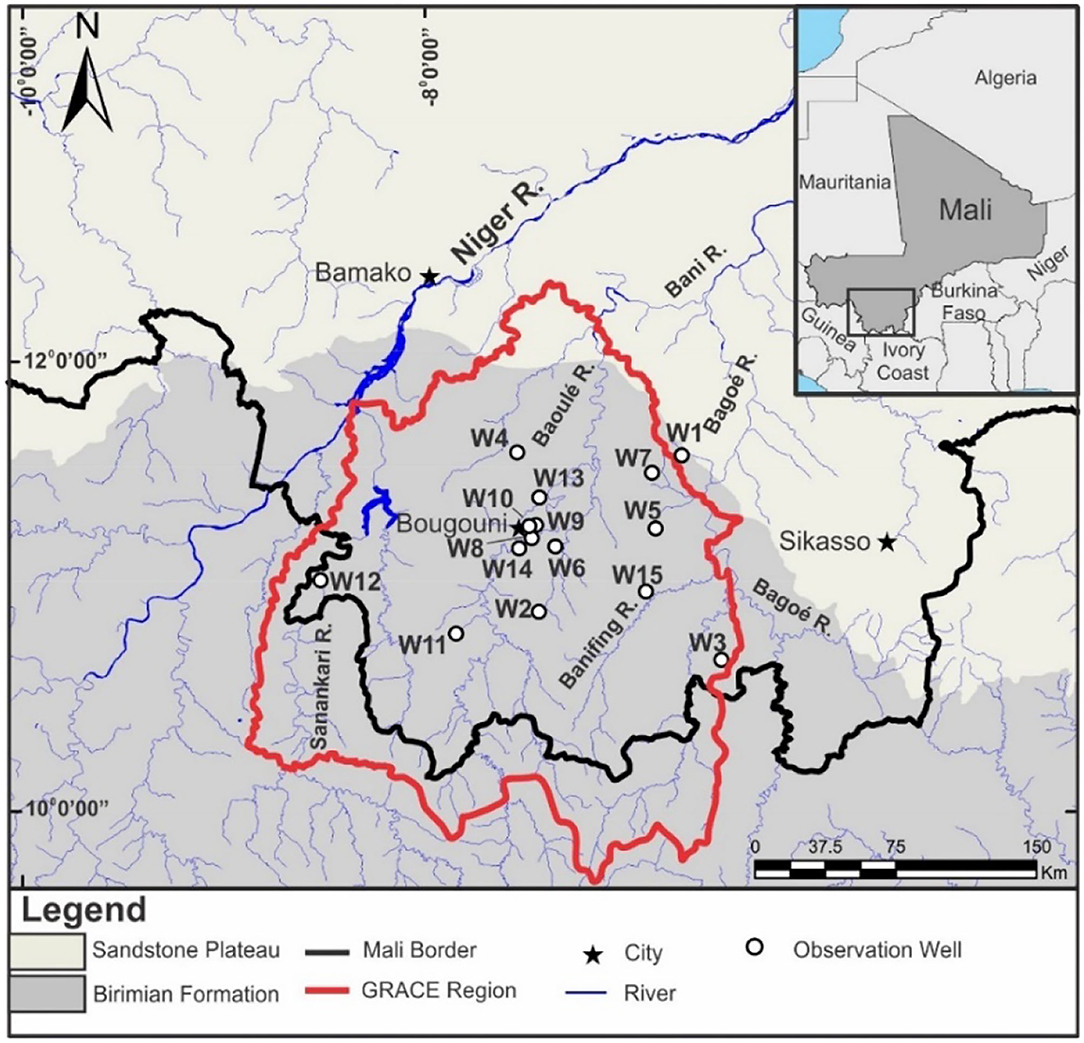
Figure 1. The study region in southern Mali showing the GRACE region (delineated with a thick red line), the observation wells (see Supplementary Table 1 for well details), and the major geological units including the Birimian Precambrian crystalline bedrock (south in gray) and the “Sandstone Plateau” Infra-Cambrian A Formation (north in beige). Insert map shows Mali in northwestern Africa.
The paper begins by presenting a conceptual model of recharge for southern Mali, based on the climate, geology and observed groundwater level records from 15 regional observation wells (Figure 1). Supplementary Table 1 shows the observation well details. Stable isotopes of groundwater samples collected in May 2008, as well as from rainwater collected in Bamako from 1962 to 1999, are used to constrain the source and timing of groundwater recharge. A series of interpretive models, thought to best represent the various recharge environments in the region based on the limited information in the available well logs, are used to simulate recharge in an exploratory manner. The simulated recharge results are averaged and compared to the timing and magnitude of recharge calculated by Henry et al. (2011) from: (1) the storage anomalies of water level records from the 15 regional observation wells, and (2) groundwater storage anomalies from Gravity Recovery And Climate Experiment (GRACE) data (1982–2002). Figure 1 shows the GRACE data region.
Materials and Methods
The Study Region
General Overview
The Republic of Mali, located in West Africa, covers an area of 1,240,000 km2 and has a population of just over 19 million (United Nations Department of Economic Social Affairs, 2019). Most of the country lies in the Sahara Desert. Southern Mali, the focus of this study, encompasses primarily the Sikasso Region to the south of the capital Bamako (Figure 1). The topography of southern Mali is generally flat with low hills (elevation 350–450 m above sea level), gentle slopes, and broad valleys. Natural vegetation consists of wooded savannas, shrublands, or grasslands of the Sudanian eco-zone (White, 1983); however, the region is increasingly cultivated. In the undisturbed areas, predominant vegetation is the wooded savanna, whereas the disturbed sites are more likely to be dominated by open shrub savannas (Tappan and McGahuey, 2007). Apart from the Niger River itself, only part of which lies in the study region just north of Bamako, the main surface water courses are its tributaries: the Sanankari, Baoulé, and Bagoé Rivers (Figure 1); all three flow northward into the Niger River.
The climate of southern Mali transitions from semi-arid near Bamako to mid-humid, sub-tropical to the south. There are three main seasons: a hot and dry period from February to May, a warm and rainy season from June to September, and a relatively cooler dry season from October to January. Average climate data (1981–2008) indicate slightly higher mean annual temperatures at Bamako (28°C) compared to Bougouni (27°C), and slightly lower annual rainfall at Bamako (879 mm) compared to Bougouni (1,044 mm) (Figure 2). Rainfall in the region is a result of the West African Monsoon, which is prone to long-term cycling between relatively wet and dry periods, although a comprehensive understanding of the intraseasonal variability remains lacking (Le Barbé et al., 2002; Janicot et al., 2011). Despite the rainy season extending over a 4- to 5-month period, precipitation events are sporadic (yet often intense) and concentrated in a period of 70–80 days (Tappan and McGahuey, 2007).
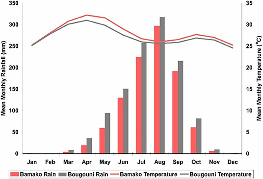
Figure 2. Average monthly rainfall (bars) and mean monthly temperature (lines) for Bamako (pink) and Bougouni (gray) as the averages from two sources (National Center for Atmospheric Research, 2009; Royal Netherlands Meteorological Institute, 2009). Period of record 1981–2008. Data from Henry (2011).
Geology
The geology of southern Mali consists predominantly of two bedrock units: the Birimian Precambrian weathered basement rock in the south and the Sandstone Plateau in the north (Figure 1). The Birimian is lithologically complex, of variable composition, and consists of metamorphosed sedimentary or igneous rocks—most commonly schists and greywackes (United Nations, 1988; ARP Développement, 2003). Overlying the Birimian are layers of sedimentary rock up to 50 m thick that consist either of poorly sorted sandstones, or more finely grained clay mineral dominated (argillaceous) sedimentary rocks (ARP Développement, 2003). The Infra-Cambrian A Formation, commonly referred to as the Sandstone Plateau is comprised of Lower Cambrian or Palaeozoic sediments and lies along the northern and eastern periphery of the Birimian (United Nations, 1988; ARP Développement, 2003). The Infra-Cambrian A is primarily comprised of sandstone, although the sandstones are sometimes inter-layered with metamorphosed clays (pelites) and Permian dolerites (British Geological Survey, 2002).
Laterites of varying ages and thicknesses commonly overlie both the Birimian and Infra-Cambrian A formations. Laterites overlying the Birimian unit more commonly have higher clay content due to the composition of the parent rock. Soils in the study region are mostly ferric luvisols, though gleyic luvisols, ferric acrisols, eutric nitosols, or lithosols are also present (Food Agricultural Organization of the United Nations, 2003; Supplementary Figure 1).
The aquifer system in southern Mali is conceptualized as consisting of a thin shallow aquifer (formed in the lateritic formations or underlying weathered bedrock zone), which overlies a relatively thick layer of argillaceous sedimentary rock overlying a fractured bedrock aquifer (Figure 3A). The shallow aquifers typically have a high porosity yet limited permeability due to the clay content of the laterite (ARP Développement, 2003). Groundwater within the shallow aquifers is obtained from traditional dug wells as the porosity is often too low to be extracted by drilled wells. The argillaceous sedimentary rock has been described as a semi-confining layer that keeps the underlying fractured bedrock aquifer hydraulically connected to the shallow aquifer through vertical or sub-vertical fractures (ARP Développement, 2003); it does not yield enough water for boreholes to be completed in it. The Birimian basement forms the fractured bedrock aquifer. Groundwater from the bedrock is pumped from drilled wells using hand or foot pumps. The productivity of the Birimian aquifers is highly variable; groundwater is most abundant where the uppermost weathered zone is thickest (United Nations, 1988; British Geological Survey, 2002). Permeability is generally low (United Nations, 1988), though dependent on the degree of fracturing (British Geological Survey, 2002). The majority of the groundwater is thought to be stored in the surface system due to its higher porosity, and drilled wells completed in the fractured bedrock indirectly exploit these reserves through hydraulic connections (ARP Développement, 2003). In Figure 3A, the borehole is shown to be cased through the soil layers, the laterite and the argillaceous sedimentary rock, and uncased in the fractured aquifer.
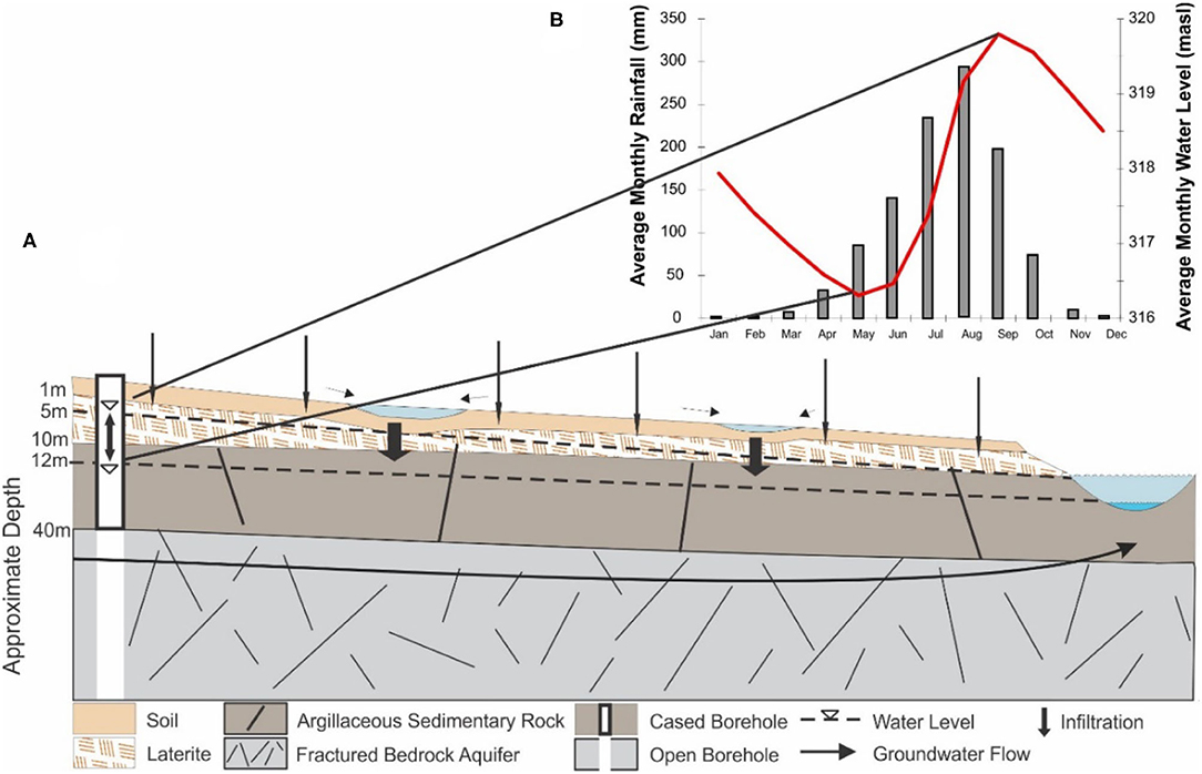
Figure 3. (A) Conceptual geological model and recharge environment in southern Mali. (B) Representative groundwater level hydrograph and regional average rainfall.
Many drilled wells in the study region underwent pumping tests following construction. In all, 805 wells were tested, of which 640 were step discharge pumping tests and 441 were constant discharge pumping tests (ARP Développement, 2003). Transmissivities for the Birimian range from 1.3 × 10⁻⁴ m2/s for granites and a diverse array of metamorphosed sedimentary rock formations (graywackes, quartzites, micaschists, gneiss, etc.) to 1.7 × 10⁻⁴ m2/s for schists, to 7.0 × 10⁻⁵ m2/s for dolorites (igneous intrusives) (ARP Développement, 2003). Specific yield (Sy) estimates for the Birimian in the study area are not available. Based on testing elsewhere in Mali and in the bordering Ivory Coast, Sy for bedrock aquifers overlain by laterite range from 0.03 to 0.07, and where the fractured bedrock is overlain by a confining layer, estimated storativity values from pumping tests range from 10−5 to 10−3 (ARP Développement, 2003). Cuthbert et al. (2019) report Sy values in the range of 0.02–0.06 for weathered metamorphic rocks in Ghana and Uganda. Henry et al. (2011) used a mid-range estimate of 0.05 for Sy for determining groundwater storage anomalies, which are compared with the recharge modeling results in this study. Section Hydraulic Properties discusses the hydraulic properties of the unsaturated zone as used in the recharge modeling.
The Recharge Environment
The climate in southern Mali consists of eight dry or relatively dry months and a 4 month long rainy season (June–September). During the rainy season, rain events occur irregularly, yet they may be very heavy when they do. Due to the aridity for most of the year, as well as the relatively impermeable clay laterite, it may be expected that much of the precipitation occurring early in the rainy season will be evapotranspired by vegetation, pool in depressions of the relatively flat topography, or runoff to nearby surface water courses where nearby (Figure 3A). As the rainy season continues, water will infiltrate the unsaturated zone directly from precipitation and perhaps locally from the pooled depressions. The laterite within the infiltration environment has a low hydraulic conductivity, is highly porous, and has a high storage capacity. These characteristics, coupled with the thickness of the unsaturated zone (~10 m deep), will cause a time lag in the response of the water table from the onset of the rainy season. However, once the infiltrating water reaches the water table, a rapid rise is expected due to the nature of the fractured aquifer at depth, which is less porous, has a lower capacity to store water, but is more permeable. The timing of the response will depend on the degree to which the shallow aquifer is in good hydraulic contact with the underlying fractured bedrock via vertical or sub-vertical fractures through the argillaceous sandstone dividing the two. In this study, it is assumed that the shallow and deep aquifer are in good hydraulic contact and that the fractured bedrock is unconfined given that the water level in the observation wells fluctuate about the laterite-sedimentary rock contact. It is possible, however, that depending on thickness and degree of fracturing of the sandstone, the confining nature of the argillaceous sedimentary rock may vary. Where thick and poorly fractured, it may act as a semi-confining layer to the fractured bedrock aquifer, and the observed water level fluctuations in the deep boreholes would be related to variations in a potentiometric surface (confined aquifer).
Water levels in the observation wells fluctuate by up to 6 m on an annual basis (Supplementary Table 1 provides the available groundwater level data for the observation wells). The groundwater level hydrographs from across southern Mali are relatively consistent, showing seasonal variations, suggesting diffuse recharge is the dominant mechanism (Cuthbert et al., 2019). The graph in Figure 3B represents the mean annual groundwater level hydrograph of all observation wells. Although significant amounts of rain historically fall in May, the water table is typically at its lowest at this time of the year; and while heavy rains have begun by June the water table rises only marginally. Not until after June does the water table begins to respond noticeably, suggesting a lag of 1–2 months from the onset of the rainy season. The rapid rise in water level caused by the low storage capacity of the fractured basement rock is evident following the heavy July rains, and peak water levels occur in September 1 month after the heaviest rain in August. The response time is thus reduced later in the rainy season from ~2 months to a few weeks. The rate of recession is related to the hydrogeology, specifically the system drainage to surface water bodies. Flow in the perennial rivers in the region is assumed to be sustained by groundwater discharge since the region is dry from November to May.
The tenets of this conceptualization of the recharge environment are examined in relation to the stable isotope data and interpretive recharge modeling results, as described in the following sections.
Stable Isotope Data
Sampling and Analysis
Twenty-three (23) groundwater samples were collected in southern Mali in May 2008, including 8 from the Birimian and 15 from the Sandstone (Figure 4). Additionally, five surface water samples were collected (Figure 4). Sample sites were crudely surveyed for geographical coordinates and elevation above mean sea level using a Magellan SporTrak portable GPS unit. If available, well-depths and well-yield estimates were recorded (Supplementary Table 2). All but two wells were hand or foot pumped; the two exceptions were hand-dug wells where water was drawn from a bucket. Wells were pumped prior to sampling to ensure the sample was representative of formation water rather than stagnant water in the hole, with three exceptions: the aforementioned two hand-dug wells, and one well that did not have a pump and was thus sampled with a clean glass bottle. Samples were stored in sealed 20 mL Nalgene bottles.
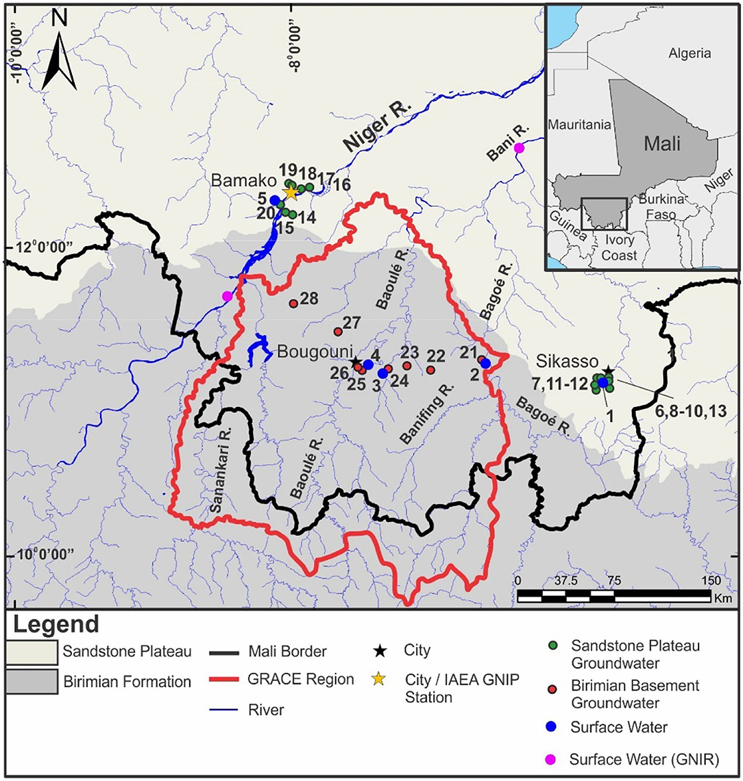
Figure 4. Location of groundwater samples in the Birimian and Sandstone Plateau and surface water samples collected in May 2008, and surface water samples from the Global Network of Isotopes in Precipitation (GNIP) for the Niger and Bani rivers.
δ2H and δ18O analysis was performed at the G.G. Hatch Stable Isotope Laboratory at the University of Ottawa using a Finnigan MAT Delta plus XP + Gasbench. Results were normalized to Vienna Standard Mean Ocean Water (VSMOW). The analytical precision was better than ± 0.04‰ for δ18O and better ± 0.58‰ for δ2H based on three blind sample duplicates.
δ2H and δ18O Content of Precipitation and Surface Waters
δ2H and δ18O isotope data for precipitation collected at Bamako (spanning 1962–1998) were obtained from the Global Network of Isotopes in Precipitation (GNIP), a joint program of the International Atomic Energy Agency (IAEA) and World Meteorological Organization (WMO) (International Atomic Energy Association, 2015). The original GNIP Bamako site was abandoned in 1998, and a new one established in 2014, with precipitation sampled until 2018. For this study only the original station data are used for consistency with the water samples collected in 2008 in this study. The reported data represent the δ2H and δ18O composition of precipitation integrated over a 1-month period, beginning on the first day of the month and continuing to the last. Data are provided with the total amount of precipitation accumulated over the 1-month period.
Mean monthly weighted δ18O and δ2H were calculated using:
where Pm is the precipitation accumulation in month m, and δ2Hm or δ18Om are the deuterium or oxygen-18 concentrations, respectively, for month m. Similarly, an integrated mean annual isotopic signature for Bamako precipitation was calculated by taking the sum of the weighted mean monthly signatures multiplied by the mean monthly precipitation accumulations, divided by the sum of the mean monthly precipitation accumulations.
In addition, a limited number of isotope data for surface waters (spanning 1990–1991) was obtained from the Global Network of Isotopes in Rivers (GNIR) for the Bani River at Douna and Niger River at Banankoro (International Atomic Energy Association, 2013) for comparison with the precipitation data, and the groundwater and surface water samples collected in this study.
Recharge Modeling
Approach
Interpretive recharge modeling was undertaken to gain insight into how geological variations might influence the rates and timing of recharge. The one-dimensional U.S. Environmental Protection Agency's HELP code (Schroeder et al., 1994) was used. HELP has been used in many recharge studies (e.g., Gogolev, 2002; Jyrkama et al., 2002; Scanlon et al., 2002b; Scibek and Allen, 2006; Jyrkama and Sykes, 2007; Toews and Allen, 2009; Allen et al., 2010; Croteau et al., 2010; Liggett and Allen, 2010; Benoit et al., 2014). It offers a practical means to explore different conceptualizations of recharge, particularly in data sparse regions, due to its low degree of parameterization. To the authors' knowledge, HELP has not been tested in a mid-humid, sub-tropical region, such as southern Mali, where rainfall is characterized by sporadic (yet often intense) events. In temperate regions, HELP appears to model recharge effectively (e.g., Gogolev, 2002; Allen et al., 2010), although in semi-arid regions it can over-estimate recharge by under-estimating evapotranspiration (Scanlon et al., 2002b; Liggett and Allen, 2010).
HELP simulates the water balance for an unsaturated column using three broad categories of data as input: a stochastically-generated daily time-series of meteorological data, unsaturated zone materials properties, and design (slope, vegetation, etc.). Infiltration into the column is calculated by subtracting runoff, surface storage, and surface evaporation from daily rainfall. Runoff is determined from a Soil Conservation Service (SCS) curve number, while surface storage and evaporation are calculated using a series of water and energy balance equations. Excess water is routed to runoff or surface storage if the calculated infiltration exceeds the storage and drainage capacity of the material. Soil evaporation and vegetative transpiration are calculated for the infiltrated water. Unsaturated vertical drainage is then computed under a unit gradient, and leakage (or recharge) through the base of the column is determined. The water table depth remains at a fixed depth throughout the simulation. Further detail regarding the HELP code's methods of solution can be found in the documentation (Schroeder et al., 1994).
Experimental Design
The dominant soil type and lithological logs from the 15 observation wells (Supplementary Table 1) were combined to create four groups of unsaturated zone columns thought to represent the main infiltration environments in the region (Figure 5). A total of 12 simulations were run. For each of the four groups, three different water table depths were considered: 5, 7.5, and 10 m below ground surface (mbgs) to reflect the range unsaturated zone depths (Supplementary Table 1). Each group was assigned different layers comprising combinations of soils, laterite, and argillaceous sedimentary rock as described below.
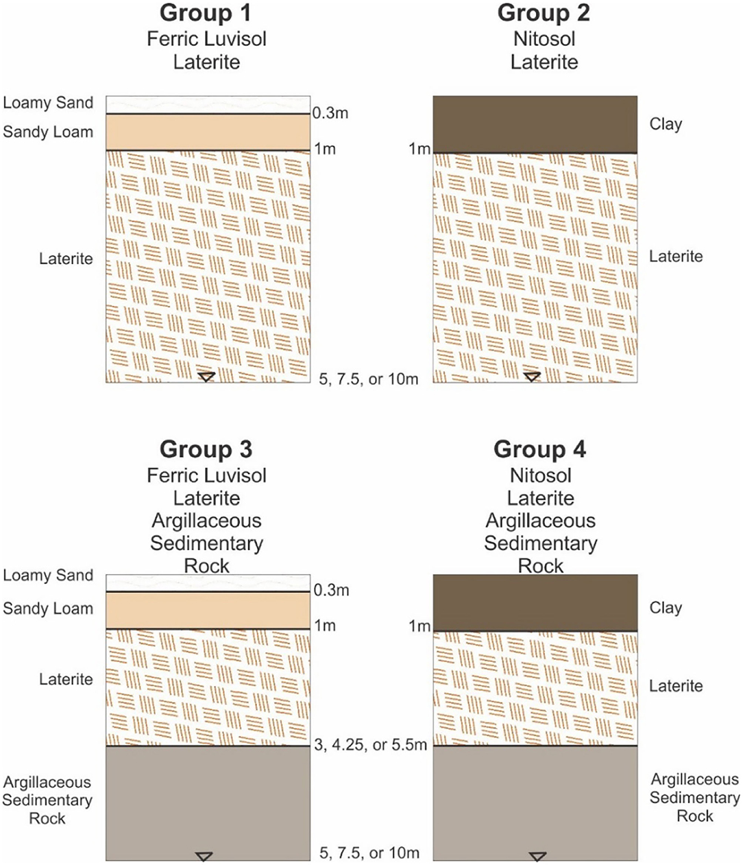
Figure 5. Conceptual models of the four unsaturated zone columns at three depth intervals (5, 7, and 10 m) thought to be most representative of the recharge environment of southern Mali based on the water levels and stratigraphy of the observation wells in the region.
Soils are assumed to be 1 m deep, with the upper 30 cm being top-soil and bottom 70 cm being sub-soil, in accordance with the world soil map produced by the (Food Agricultural Organization of the United Nations, 2003) (Supplementary Figure 1). Only the ferric luvisol and nitosol soils were considered for representing the soil horizon in the models, as these are the most abundant in the region and the properties of the other soils are within the spectrum between these two soil types. Ferric luvisol is a predominantly sandy soil, with 82% of the topsoil and 75% of the sub-soil being sand. Conversely, the nitosols are predominantly clay dominated, with ~60% of the topsoil and 70% of the sub-soil being clay for both the dystric and eutric nitosols (Food Agricultural Organization of the United Nations, 2003). The compositions of the top- and sub-soils for both the ferric luvisol and nitosol were classified into soil textures according Dingman (2002, Figures 6-3). The ferric luvisol top-soil thus has the texture of a loamy sand, while the sub-soil has a sandy loam texture, and is represented in Groups 1 and 3. The top- and sub-soils of both the dystric and eutric nitosols are classified as clay and are represented by one layer in Groups 2 and 4 (Figure 5).
Beneath the soil horizon, two scenarios were considered (Figure 5): (1) the entirety of the column is laterite (Groups 1 and 2), and (2) the remainder of the column is split evenly between laterite that overlies argillaceous sedimentary rock (Groups 3 and 4).
Hydraulic Properties
Estimates of saturated hydraulic conductivity (Ksat) for the soils were obtained from Dingman (2002, Tables 6-1) and for total porosity, wilting point and field capacity were chosen as the mid-point of the ranges shown in Dingman (2002, Figures 6-4) (Table 1).
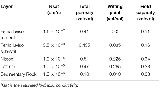
Table 1. Hydraulic properties for each layer of unsaturated zone material.
There are no estimates of the hydraulic properties of laterite in southern Mali. The Ksat of laterite is dependent on a number of factors, including the degree of weathering and the presence or absence of fractures or other macropores. Ksat values in literature range from 4.6 × 10⁻² cm/s (obtained from one of 106 infiltration tests of a lateritic catchment in Western Australia; Sharma et al., 1987) to 1.0 × 10⁻⁶ cm/s (from near the base of a laterite profile in Kerala in southwest India; Langsholt, 1992). Langsholt (1992) found that the Ksat for laterite ranged from ~1.0 × 10⁻² to 1.0 × 10⁻⁶ cm/s in the same profile between its top (higher Ksat) and its base (lower Ksat). As discussed in Section Geology, the laterite layer in southern Mali has a relatively low hydraulic conductivity and a high porosity. Therefore, the Ksat value for laterite was set to 1.0 × 10⁻⁵ cm/s and the porosity 0.47 (Table 1). Kew and Gilkes (2006) found clay-rich lateritic regolith in Western Australia had the highest water-retention characteristics amongst eight other regolith materials. Therefore, values of 0.265 and 0.38 were used for wilting point and field capacity, respectively.
The argillaceous sedimentary rock overlying the fractured bedrock is assumed to have a low hydraulic conductivity, but one high enough to allow water to pass between the laterite and fractured bedrock. Therefore, Ksat was set to 1.0 × 10⁻⁶ cm/s and the porosity 0.10 (Table 1). It was also assumed that the argillaceous sedimentary rock layer has poor moisture retention characteristics; thus, the wilting point and field capacity were set at the low values of 0.013 and 0.03, respectively. Given the uncertainties in the hydraulic properties of the argillaceous sedimentary rock a sensitivity analysis was conducted (see Section Model Calibration and Sensitivity Analysis).
Climate Parameters
The HELP code includes a weather generator (WGEN; Richardson and Wright, 1984) for simulating a daily stochastic weather series for input to the model. The weather generator uses monthly climate parameters (e.g., mean daily temperature, precipitation, and solar radiation), quarterly relative humidity, and a variety of statistical parameters that describe the precipitation distribution, occurrence of wet vs. dry days, etc.); WGEN includes a database of these statistical parameters for many climate stations around the world. The closest climate station listed in the weather generator database in southern Mali is Bamako. The monthly normals for mean daily temperature and precipitation in the database were adjusted to reflect the observed climate data used in this study from National Center for Atmospheric Research (2009) and Royal Netherlands Meteorological Institute (2009), which were averaged and used as input (Table 2). Relative quarterly humidity was obtained from the British Broadcasting Corporation (BBC) Weather Center (British Broadcasting Corporation, 2010). The other climate statistical parameters were left as the default values in the database (Table 2).
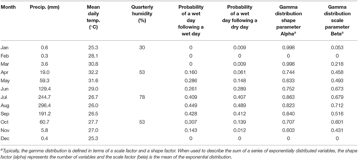
Table 2. Climate parameters used for weather generation.
Evapotranspiration Parameters
Temperature, relative humidity, wind speed, leaf area index (LAI), growing season length, and evaporative zone depth are used in the calculation of actual evapotranspiration (AET). LAI was estimated from several studies, notably the HAPEX (Hydrology-Atmosphere Pilot Experiment)—Sahel experiment, which was undertaken in the southern Sahel of neighboring Niger (Goutorbe et al., 1994; Prince et al., 1995). Vegetation at one fallow savanna site of the experiment consisted of small (1–3 m) shrubs (Guiera senegalensis) with a canopy cover of about 8% underlain by a continuous layer of annual grasses (Hanan et al., 1996). It was found that LAI averaged only 0.24 for the shrubs and 0.12 for the grass layer. Rapidel et al. (2006) showed that maximum LAI varied amongst six vegetation classes, between 1.3 and 3.3, and that the time that the LAI exceeds 1 is short, varying between just 37 and 86 days. These short time periods are relatively consistent with the short growing season period (59 days; Table 3). Therefore, a maximum LAI of 0 was used in these simulations. However, maximum LAI was explored in the sensitivity analysis.
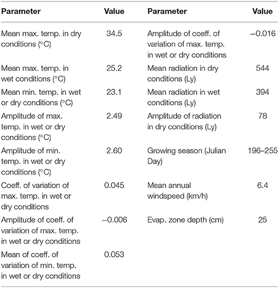
Table 3. Additional default parameters for Bamako in the weather generator.
The evaporative zone depth (EZD) is the depth to which water can be removed from the column by evaporation or transpiration (Schroeder et al., 1994). Three options are available: 25 cm for bare soil, 56 cm for a fair stand of grass, and 102 cm for an excellent stand of grass. The EZD was set to 25 cm in accordance with the LAI of 0 and generally bare soil conditions (Table 3). Accordingly, vegetation class was set to bare ground. Thus, the model represents a case of very low evapotranspiration. Observations in the field during May of 2008 confirms such low LAI values given the sparse vegetation and predominantly bare ground. However, EZD was explored in the sensitivity analysis for low, moderate, and high evapotranspiration scenarios.
Surface Water and Initial Moisture Settings
Runoff is calculated in HELP using the Soil Conservation Service (SCS) Curve Number (CN) where a maximum CN of 100 occurs when there is no runoff. As no CN estimate was available for the study region, the runoff method used in these simulations was model-calculated CN. The runoff area (the percentage of the surface that allows runoff) was set to 100%, and the slope set to zero to reflect the generally flat topography of the region. However, the effect of slope was considered in a sensitivity analysis.
The initial moisture was set to model-calculated, whereby HELP assigns realistic initial moisture storage values for each layer and simulates the water balance for 1 year (Schroeder et al., 1994). The layer's moisture content at the end of that year is then used as the initial moisture storage for the next year. Model output was only examined for the last 30 years of a 100-year simulation to allow for sufficient model spin up time. Therefore, the initial moisture content is not a concern.
Model Calibration and Sensitivity Analysis
The recharge models are interpretive and so were not subject to calibration. Therefore, a sensitivity analysis was performed to determine the effect of (1) maximum LAI, vegetation class, and evaporative zone depth, (2) slope, and (3) the uncertain hydraulic properties of the argillaceous sedimentary rock unit of Groups 3 and 4.
For each of Groups 1 and 2 (representing the two main soil types) for column depths of 7.5 m, three scenarios of varying evapotranspiration parameters were considered:
• Low AET scenario—maximum LAI = 1, vegetation class = poor stand of grass, evaporative zone depth = 25 cm
• Moderate AET scenario—maximum LAI = 3, vegetation class = fair stand of grass, evaporative zone depth = 56 cm
• High AET scenario—maximum LAI = 5, vegetation class = excellent stand of grass, evaporative zone depth = 102 cm
All other input data were left the same as the input parameters for Groups 1 and 2.
The sensitivity analysis for slope was conducted Groups 1 and 2 for 7.5 m column depths:
• “Flat” —slope = 5% and slope length = 10 m
• “Rolling” —slope = 15% and slope length = 10 m
The sensitivity analysis for the argillaceous sandstone considered an alternative conceptualization of a more weathered material (i.e., argillaceous regolith material as opposed to structurally in-tact rock), with properties similar to the regolith studied in Western Australia by Kew and Gilkes (2006). Five scenarios were considered (the base model used a Ksat = 1.0 × 10⁻⁶ cm/s):
• Ksat = 1.0 × 10⁻³ cm/s, porosity = 0.10, wilting point = 0.013, field capacity = 0.03
• Ksat = 1.0 × 10⁻⁵ cm/s, as above
• Ksat = 1.0 × 10⁻⁷ cm/s, as above
• Ksat = 1.0 × 10⁻⁶ cm/s (base model value), porosity = 0.47, wilting point = 0.265, field capacity = 0.378
• Ksat 1.0 × 10⁻⁶ cm/s, porosity = 0.40, wilting point = 0.024, field capacity = 0.062.
Recharge Estimation From Observed Storage Anomalies
Henry et al. (2011) estimated recharge using the water table fluctuation (WTF) method (Healy and Cook, 2002):
where R is recharge, Sy is specific yield, Δh is the change in the height of the water table and Δt is the time interval. In this instance, Δh is the difference between the peak and trough measured at an annual timestep on a water level hydrograph. Henry et al. used a Sy value of 0.05.
Cuthbert (2010, 2014) proposed that system drainage rate (D) should be accounted for in the WTF method:
where D can be estimated for each hydrograph using the steepest recession observed during a period where there is little recharge. This drainage term accounts for the fact that as the aquifer is being replenished it is continually draining, and so the water level does not reach as high a peak as it would if there were no drainage.
Accordingly, the mean annual hydrographs for all 15 observation wells were re-analyzed in this study to correct for D. The months of November to March have essentially no precipitation (Figure 2); therefore, the difference in water level over this 5-month period was multiplied by Sy to obtain D for each well. Ideally, the drainage should be calculated for each year to account for interannual variability; however, for simplicity D was estimated using the average annual hydrograph for each well, over a period of 5 months (November–March). The same Sy value of 0.05 as used by Henry et al. (2011) was also used, but in addition, a range of Sy values (0.02–0.07) for similar settings and rock type were explored.
Results
Stable Isotopes
The isotope results are provided in Supplementary Table 2. The weighted mean monthly (12 discrete points) and mean annual (single point) δ18O and δ2H of Bamako precipitation (δ2H = 6.15δ18O – 0.49; R2 = 0.97) are plotted in Figure 6, along with the isotopic composition of the groundwater samples (δ2H = 7.43δ18O + 1.55; R2 = 0.93), distinguished as being sampled from the Sandstone and the Birimian, and the surface waters sampled in this study (δ2H = 3.41δ18O – 7.12; R2 = 0.84).
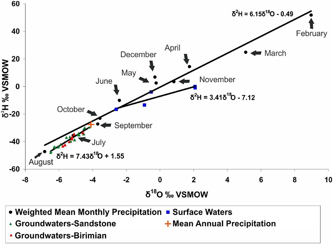
Figure 6. Weighted mean monthly and mean annual δ18O and δ2H signatures of Bamako precipitation, with the δ18O and δ2H content of groundwaters in the Sandstone and Birimian, and surface waters sampled in May of 2008.
Rainfall occurring earlier in the year is the most isotopically enriched (Figure 6). Note that there is no value for January because no precipitation events occurred in that month throughout the period of record (1962–1998). As the rainy season begins (in May/June), the precipitation gradually becomes more isotopically depleted, with the most depleted rainfall occurring in August (which is also historically the wettest month). Following August, the precipitation becomes more enriched. Supplementary Figure 2 shows the isotopic composition of monthly precipitation (from GNIP); notably there are some precipitation samples (mostly August values) that are more depleted than the weighted mean monthly value for August.
All of the groundwater samples (collected in May) exhibit isotopic signatures within the range of July, August, and September precipitation. These results suggest two things: (1) groundwater is of meteoric origin, and (2) the majority of groundwater recharge is derived from rainfall during these months. This result was somewhat unexpected because the rainy season begins in May/June, and rainfall during these months was expected to contribute to recharge. One possible explanation for the lack of a May-June isotopic composition for groundwater recharge is that the annual isotopic signature of precipitation is dominated by July-August-September rainfall (71% of annual Bamako rainfall on average), such that it likewise affects the groundwater composition. However, the mean annual isotopic signature, which integrates precipitation over all months, is slightly more enriched than any of the groundwater samples (see + symbol in Figure 6), suggesting that early rainy-season rainfall may contribute little to recharge. This may be due to the soil zone being desiccated at the end of the dry season such that the majority of precipitation occurring early in the rainy season is lost to evaporation during depression storage or is evapotranspired from what little vegetation exists. Alternatively, the groundwater isotopic compositions may reflect mixing between early summer and late summer precipitation.
The five surface waters sampled in this study are more enriched, particularly in δ18O, compared to the local meteoric water line (Figure 6). The slope of the surface water samples is indicative of water that has undergone evaporation under low-humidity conditions (0–25%; Clark and Fritz, 1997). This is reasonable in consideration of the time of sampling—May, a transition month from the dry to rainy seasons—which follows a long, dry period. For comparison, Supplementary Figure 3 shows the isotopic composition of the Bani and Niger rivers in 1990–1991 (from GNIR; see Figure 4 for sampling locations) alongside the surface waters sampled in this study in May 2008.
Recharge Modeling Results
Annual Water Budget
The annual water budget results for the last 30 years of the simulation were compiled for each of the 12 column simulations. The results are arranged in Supplementary Table 3 by group and unsaturated zone depth (5, 7.5, and 10 mbgs) (see Figure 5). Climate is the same for all 12 simulations. Rainfall varied over the 30 years between 712 and 1,418 mm/yr, with an average of 1,027 ± 147.8 mm/yr. Runoff and actual evapotranspiration (AET) are the same at all depths for groups with the same soils (i.e., Groups 1 and 3 which have ferric luvisol soils, and Groups 2 and 4 which have nitosol). A small amount of runoff occurs in the groups with nitosol soils; the clayey nitosol has a sufficiently low permeability to generate runoff if there is enough rainfall, even in the absence of topographic slope. Average, runoff was ~6 mm/yr (or 0.6% of annual rainfall) in these groups, ranging from 0 to 70.8 mm/yr.
AET did not vary amongst groups with the same soils because the soils are deeper (at 1 m) than the evaporative zone depth (25 cm). In Groups 1 and 3 with the sandier ferric luvisol soil, AET ranged from 338 to 632 mm/yr, averaging 465 ± 68 mm/yr (46% of rainfall). In Groups 2 and 4, AET ranged from 401 to 723 mm/yr, averaging 534 ± 72 mm/yr (53% of rainfall). More water was evapotranspired in the groups with the nitosol soil since the high clay content stores more water and does not transmit it downward as quickly as the sandier ferric luvisol.
The total amount of recharge (R) amongst each group varied little with column depth, with average amounts being greater by ~3–4 mm/yr in the 10 m deep columns than the 5 m deep ones. This is likely because during the 30-year simulation period the amount of water stored (S) within the columns remains constant (the highest standard deviation of soil water storage in any simulation is 0.01). Thus, the only factor affecting recharge from year to year is the amount of precipitation that infiltrates the surface without evapotranspiring, pushing the water held in storage through the bottom layer (piston flow). Rather, the effect of depth on recharge is evident in the timing and the amount of recharge amplitude (as the difference between the highest and lowest monthly recharge amounts), as discussed later.
Average annual recharge ranged from 552 to 555 mm/yr for Group 1 and 557 to 560 mm/yr for Group 3, while for Groups 2 and 4, recharge ranged from 478 to 482 mm/yr and 483 to 486 mm/yr, respectively. The ranges and standard deviations for annual recharge amounts are high for all 12 simulations, reflecting the variability of the precipitation (Supplementary Table 3). With respect to the influence of the layers' hydraulic properties of each group on recharge, two general observations can be made from the annual water budget: (1) in Groups 1 and 3 with ferric luvisol soil, more water percolates through the bottom layer than Groups 2 and 4 with nitosol soil, and 2) Groups 3 and 4 with 50% sedimentary rock underlying the 1 m soil layer experienced slightly more recharge than Groups 1 and 2 with only laterite beneath the soil layer. The difference in recharge between groups that have ferric luvisol rather than nitosol soil is ~70 mm/yr, while the difference between those groups that have sedimentary rock present and those that are only laterite below the soil is only 5–6 mm/yr. Thus, the presence of the top 1 m soil layer exerts a much greater influence on annual recharge amounts than the presence or absence of sedimentary rock.
Monthly Recharge
Mean monthly simulated recharge graphs were created by averaging the recharge for each month for all 30 years (Figure 7). While the average annual simulated recharge was approximately the same for all three depth simulations within a group (Supplementary Table 3), the timing of recharge throughout the year was affected by the depth of the column, such that the recharge response was delayed with increasing column depth.
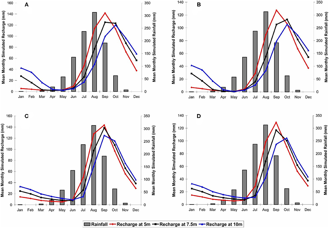
Figure 7. Mean monthly recharge (left y-axis) and mean monthly precipitation (right y-axis) at three depths for 30 years of simulation for (A) Group 1, (B) Group 2, (C) Group 3, and (D) Group 4.
A composite graph of mean monthly simulated recharge for all simulations was generated by averaging the results from the 12 simulations (Figure 8). By incorporating the stratigraphic sequences of all four groups, this composite graph encompasses all the principal recharge scenarios that typically occur in the study area, thereby enabling a comparison with the regional groundwater level storage anomaly and GRACE satellite results from Henry et al. (2011), as discussed later. The peak recharge for this composite plot occurs in September, 1 month after the heaviest rains in August (Figure 8). The lowest monthly recharge occurs in May, although the graph shows nearly as little recharge from April through June. The recharge response starts in July, 1 month after the arrival of the rainy season, and recharge is greatly accelerated through August to its peak in September. Monthly recharge is still very high in October, and then recession occurs rapidly up to December. Continued recession—from January on—occurs more slowly.
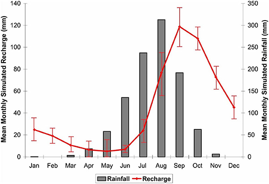
Figure 8. Mean monthly precipitation (right axis) and recharge (left axis) for the average of all four groups at all three depth intervals (12 simulations). Standard deviation shown as bars.
Sensitivity Analysis
The results of the sensitivity analysis for evapotranspiration parameters are provided in Supplementary Table 4. In the following summary, percentages are with respect to the annual simulated rainfall and relative to base model [very low AET scenario: LAI set to 0, vegetation class set to “bare ground,” and an evaporative zone depth (EZD) of 25 cm]. The sensitivity analysis showed that there was minimal impact on the annual water balance under a “low AET” scenario with the maximum LAI set to 1, vegetation class set to “poor stand of grass,” and an EZD of 25 cm for columns with either ferric luvisol (Group 1) or nitosol (Group 2) soils. The columns with ferric luvisol soils were slightly more sensitive to the evapotranspiration parameters than those with nitosol soils. A “moderate AET” scenario (maximum LAI of 3, vegetation class of “fair stand of grass,” EZD of 56 cm) increased annual AET and decreased recharge for the columns with ferric luvisol soils by 9.4%, while AET increased by 3.7% and recharge decreased by 3.1% for the nitosol-soil columns. In the ferric luvisol columns, the “moderate AET” scenario shifted the monthly recharge peak 1 month later. In columns of either soil type, there was little difference between the moderate AET scenario and the “high AET” scenario (maximum LAI of 5, vegetation class of ‘excellent stand of grass', EZD of 102 cm), although the high AET scenario did shift the monthly recharge peak of the nitosol columns later by 1 month. Given that there is little difference between the low AET and base model scenarios, it is concluded that AET is simulated adequately by HELP for the study region.
The sensitivity analysis for slope showed that columns with ferric luvisol are moderately impacted by the presence of a gentle slope, while columns with nitosol soil are strongly affected (Supplementary Table 5). A 10 m long slope of 5% increases annual runoff by 7.5% and decreases annual recharge by 8% in the ferric luvisol columns, as well as shifts the monthly recharge peak later by 1 month. For the less permeable nitosol columns, the same slope scenario increases annual runoff of the by 31.8% and decreases annual recharge by 29.7%, shifting the monthly recharge peak by 1 month. Increasing the slope to 15% had little effect on columns with either soil type, as the results were largely similar to the simulations at a slope of 5%. The slope simulations did not noticeably alter the AET calculated by HELP, as the effect on the water budget was observed only in runoff and recharge variations. Introducing a slope to the model therefore could reduce the simulated recharge 8 to 30%. However, the generated runoff would likely accumulate in small topographic depressions and infiltrate unless evaporated.
The sensitivity analysis also tested the effect of various saturated hydraulic conductivities and water retention characteristics of the argillaceous sedimentary rock unit. The results (see Henry, 2011) showed that no change to any of these parameters affected the amount of annual recharge totals. A slight impact on the timing of monthly recharge was observed—for instance, a very low hydraulic conductivity of 1.0 × 10⁻⁷ cm/s caused a more rapid response of recharge to rainfall and more rapid drainage, while increasing the water retention characteristics to those more representative of clay or laterite caused a slower response of recharge to rainfall and slower drainage. These changes to the timing of recharge can alter the amount of average annual recharge amplitude by up to 1.9%. However, overall the sensitivity analysis showed that there was minimal impact of the sedimentary rock hydraulic parameters on the recharge results, and these are not considered to be a great source of uncertainty.
Discussion
Isotopic Evidence in Support of Recharge Source and Timing
The δ2H and δ18O isotopes show groundwater samples plotting within the range of the weighted mean monthly δ18O and δ2H concentrations of July-August-September rainfall, and below the weighted mean annual δ18O and δ2H signal for precipitation in Bamako (Figure 6). This strongly suggests that the source of recharge is July to September rainfall. If the groundwater were recharged from precipitation from all months, the samples should cluster about the mean annual isotopic signature of precipitation, because the annual composition is weighted according to monthly precipitation amount.
Jasechko and Taylor (2015) evaluated δ18O and δ2H in rainfall and groundwater in tropical regions throughout the world, including Bamako, and found that groundwater recharge is dominated by high-intensity rainfall events. While this study did not explicitly examine the association between rainfall intensity and the isotopic compositions of rainwater and groundwater, the rainy season (from June to September) is characterized by sporadic and often intense precipitation events (Tappan and McGahuey, 2007). These months have the greatest rainfall amounts, with 72% (742 mm) of the simulated annual rainfall (1,027 mm) falling in the months of July, August, and September. The recharge modeling suggests that, on average across all 12 simulations, 303.7 mm of recharge occurs during the months of August, September and October, accounting for 58.5% of the total 519.0 mm that recharges annually.
Comparing Simulated Recharge With Storage Anomalies From Observation Wells and GRACE Satellite Data
One of the goals of this study was to compare the simulated recharge results to the timing and magnitude of recharge calculated from the storage anomalies of the observed regional water level records and GRACE. Before delving into this comparison, it is important to acknowledge that the storage anomaly datasets (from both the observation wells and GRACE) are not directly comparable with the recharge modeling results. The HELP simulations give estimates of recharge as the amount of water percolating through the bottom layer of the unsaturated zone. HELP does not directly simulate fluctuations of the water table; rather it simulates the net water input to the saturated groundwater system at the base of the unsaturated zone. The water table is assumed to remain at a constant depth throughout the simulation as defined by the base of the column. An unmovable water table depth is not considered a limitation in this study because the water table historically remained below surface (>1 m) in all observation wells, allowing for continued infiltration. In contrast, the observed storage anomaly records are based on measurements of the water level fluctuation within the fractured rock aquifer. These are converted to a storage anomaly by multiplying the regionally averaged groundwater level anomaly by Sy following a similar approach to Rodell et al. (2007) and Strassberg et al. (2009). Henry et al. (2011) used a value of Sy = 0.05, acknowledging the uncertainty in this value. Terrestrial water storage (TWS) anomalies from GRACE data, which were corrected for soil moisture (SM) variations using the Global Land Data Assimilation System (GLDAS) model, represent monthly groundwater storage anomalies (GRACE minus SM) (details on the approach can be found in Henry et al., 2011). Thus, the GRACE—SM also reflect changes in groundwater storage, and not recharge. Nevertheless, similarities between the recharge response and the storage anomalies can be expected if the simulations are sufficiently realistic and some assumptions are made. Particularly, the response of the storage anomaly hydrographs to recharge should correspond to the timing of simulated recharge events. The recharge amount should also be similar if the Sy used to calculate the storage fluctuations and the hydraulic parameters of the unsaturated zone assigned in the simulations are realistic.
Figure 9 (modified from Figure 7 in Henry et al., 2011) shows the observed monthly groundwater storage anomaly over the period of available data (1982–2002) plotted as the regional average of the 15 observation wells (see Figure 1 for well locations), and the monthly storage anomalies of GRACE TWS, modeled soil water storage (SM), and interpreted groundwater storage (GRACE – SM) for the period 2002–2008. The monthly storage anomalies fluctuate consistently about the 0 mm mark by ±~75 mm. The decrease in groundwater storage observed prior to 1985 may not be representative, as this portion of the record is based on only three wells. Otherwise, no long-term trends are evident.
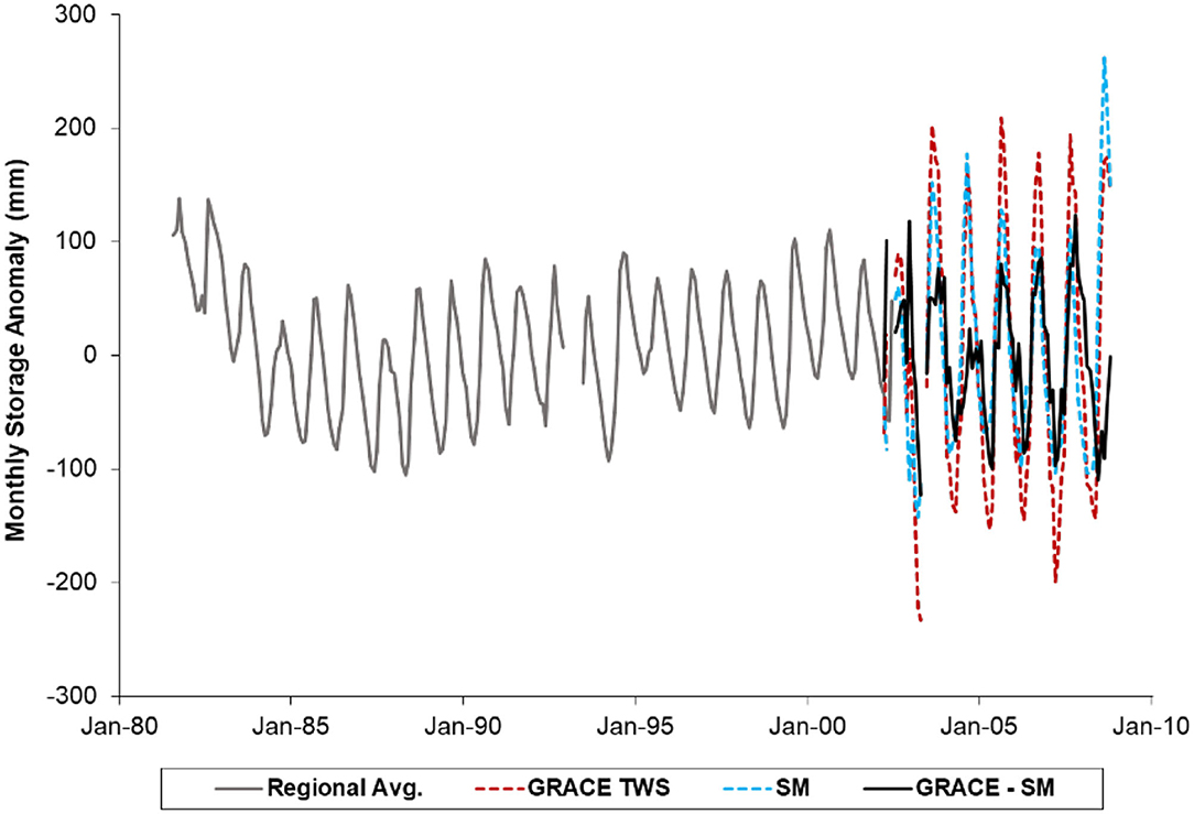
Figure 9. Mean monthly storage anomaly hydrographs of the regionally averaged observed groundwater storage (1982–2002), GRACE measured TWS (2002–2008), GLDAS predicted SM (2002–2008), and interpreted GRACE – SM groundwater storage (2002–2008).
Recharge results were first compared by recharge group. Mean monthly simulated recharge graphs were generated for the 12 simulations (4 groups with 3 water table depths) by averaging the recharge amounts for each month for all 30 years. The simulated recharge for each of the three depths are shown in Figure 10 (the same graphs are shown in Figure 7) along with the observed storage anomaly hydrographs for individual wells within each group. Importantly, the primary and secondary y-axis scales are not the same, so the amplitudes should not be compared, just the pattern. It is clear from Figure 10 that there is considerable variability among the storage anomaly hydrographs within each group. This is because the groundwater system is heterogeneous and the properties of the fractured aquifer and unsaturated zone at individual well locations are variable. In contrast, the simulations were designed to generalize this complex recharge environment based on the stratigraphy of the observation well logs, water level depth, and soil cover.
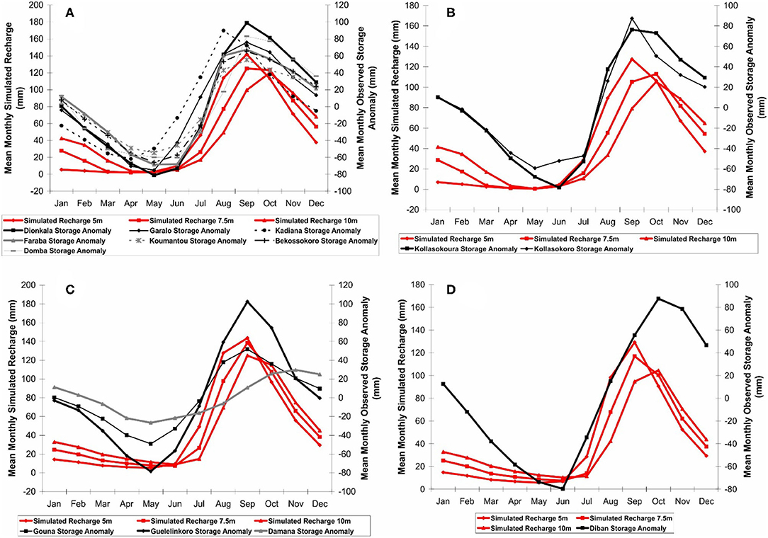
Figure 10. Mean monthly simulated recharge (left y-axis) and mean monthly storage anomalies (right y-axis) for observation wells characteristic of (A) Group 1, (B) Group 2, (C) Group 3, and (D) Group 4.
To regionalize the simulated recharge results, the 12 individual recharge simulation results were combined to determine the regional recharge response, and this regional response was compared to the regional observed and GRACE—SM storage anomaly hydrographs as shown in Figure 11.
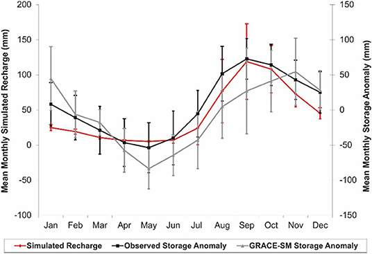
Figure 11. Mean monthly simulated recharge for the average of all four unsaturated zone groups at three depth intervals (12 simulations) (left y-axis), with the mean monthly storage anomalies for the entire region compiled from all observation wells and interpreted groundwater storage GRACE – SM (right y-axis). Error bars represent the standard deviation in each dataset.
Overall, there is generally good agreement between the timing and magnitude of the mean monthly simulated recharge and the regional mean monthly storage anomaly hydrograph generated from all observation wells (Figure 11). The troughs and peaks of both the modeled recharge and regional observed storage anomaly curves occur in May and September, respectively. The initial response to rainfall occurs somewhat earlier in the observed regional storage curve than in the simulated recharge results, as the rise from May to June and from June to July is more significant. However, following the initial response, both curves rise through the rainy season at a similar rate, peaking in September. The initial recession following the peak (up to December) is similar as well, although the drainage from the HELP unsaturated zone columns occurs a little more rapidly and there is a greater reduction in monthly recharge in this period than there is a storage loss. In the dry season, during the early part of the year, the regional observed storage loss continues due to drainage within the groundwater system. The apparent “flatline” simulated recharge response during the late recession (from March to June) is caused by the unsaturated column having no further stored water to continue to provide recharge to the deeper groundwater system. Thus, recharge approaches and remains close to zero. These flatline recharge responses are particularly evident for the shallowest water table simulations at 5 m (see Figure 10).
The GRACE – SM storage anomalies do not, however, compare well with the regional observed monthly storage anomalies and the recharge simulations (Figure 11). All experience lows in May and show similar initial response to rainfall, with increases in recharge amount or storage anomaly of ~70–100 mm between May to August. However, the GRACE – SM curve continues to rise steadily at a lower rate after August, peaking in November, 2 months later than the modeled and observed peak. Following the peak, the loss of groundwater storage seen in GRACE – SM is much faster and more significant than the recession of observed storage anomaly. Henry et al. (2011) concluded that the GLDAS land surface model used to estimate changes in soil moisture storage poorly resolved the timing of the soil moisture storage changes, despite a strong correlation between the GRACE total water storage (TWS) changes and the observed regional storage anomalies.
Comparing Simulated Recharge Other Recharge Estimates
MacDonald et al. (2021) place the region of southern Mali in a recharge range of 100–250 mm/yr based on recharge estimates reported in various studies and using a variety of methods from across Africa; note that the field study cited for southern Mali is Henry et al. (2011). As described in Section Recharge Estimation from Observed Storage Anomalies, Henry et al. (2011) estimated annual recharge as the difference between mean monthly storage anomaly peaks and troughs but did not account for drainage in the WTF method (Equation 3). They reported an average annual historical (1982–2002) recharge from the observed storage anomalies at 149.1 mm (or 16.4% of annual rainfall), and from the interpreted GRACE–derived recharge (2002–2008) at 149.7 mm (or 14.8% of annual rainfall. If drainage is accounted for (Equation 4), and using a Sy value of 0.05, recharge from the observed storage anomalies ranged from 189 to 619 mm/yr (ave. 384 mm/yr). For comparison, in neighboring Burkina Faso (a similar climate region), a study using the WTF method gave a recharge range of 160–400 (ave. 266 mm/yr) (Filippi et al., 1990).
Henry et al. (2011) argued that an Sy value of 0.05 gave the best match to the GRACE – SM storage anomaly amplitudes and thus considered it a realistic value for the entire region. However, to address uncertainty in Sy, a range of Sy values is considered here. Using Sy = 0.02, recharge from the observed storage anomalies ranged from 83 to 390 mm/yr (ave. 243 mm/yr), and using Sy = 0.07, recharge ranged from 233 to 772 mm/yr (ave. 478 mm/yr). Thus, the full range of uncertainty in recharge estimated from the observed storage anomalies is 83–772 mm/year due to uncertainty in Sy, and the regional average annual simulated recharge is 519 mm/yr (479–560 mm/yr range among the 12 models).
Limitations
There are several main limitations to this study. First, is that the water level records were all acquired from boreholes completed in the fractured bedrock aquifer of the Birimian basement, and it was assumed that water table fluctuations coincide with fluctuations in the water level for the deep aquifer. However, both the timing and magnitude of the fluctuations may differ due to the physical separation (via the sandstone) between the fractured aquifer and the shallow aquifer and the potential for the sandstone to act as a semi-confining unit. While it is assumed that the shallow and deep systems are in close connection, if the sandstone does function as a semi-confining layer, a potentiometric response in the deeper aquifer could be delayed relative to the water table response. This scenario would also invalidate the WTF method as it is intended for use in unconfined aquifers. However, the water levels in the observation wells do fluctuate about the laterite-sedimentary rock contact suggesting unconfined conditions.
The observed water level fluctuations may also be influenced by factors other than recharge. Ideally, observation wells used for recharge analysis should be situated in recharge areas, up-gradient from any boundary effects. For example, the water level in observation wells situated nearby streams may be influenced by stream levels, rising at times of the year when streamflow is high. Nearby pumping can lower groundwater levels, while irrigation can raise the water table. In this study, it is assumed that the observation wells are not to be influenced by these factors.
Given the lack of data with which to parameterize the models, some uncertainty in the modeling results is inevitable. The interpretive modeling approach attempted to use the best (or only) estimates of hydraulic properties for the material types present. There are also uncertainties related to the parameters needed for the calculation of actual evapotranspiration (AET); maximum LAI, vegetation class, and evaporative zone depth. The sensitivity analysis suggested that the evapotranspiration settings were reasonable. Slope, however, was shown to be important. Even a gentle slope can have large effect on recharge amounts, especially if the soil has a high clay content, because considerably more runoff is generated. Recharge could be reduced by as much as 30% if a 5% slope is introduced with a clay soil. The one-dimensional columns used for the recharge modeling were assigned a zero slope so as to maximize infiltration. However, if a slope had been assigned in the one-dimensional models the simulated recharge would have been reduced by up to 30%. This suggests that the average simulated recharge would be 363 rather than 519 mm/yr. However, even if slope were assigned in the models, the runoff process would not be captured using a one-dimensional recharge model—i.e., the model does not route surface water runoff.
So, why then was a fully integrated land surface—subsurface regional scale model not used in this study? Such a model would incorporate topographic variations and enable infiltration excess overland flow to be routed to streams; although, the small scale variations in topography associated with depression-focused recharge would not be captured in a regional scale model. Indeed, to compare groundwater storage anomalies averaged over a region of a suitable size for GRACE, a regional scale hydrological model would be needed. The problem is that such models are highly parameterized and require a good observational dataset for calibration. Even for this study, estimates of most of the model parameters had to be estimated from the literature. Thus, there was a need to explore how local variations in geological materials, specifically the layering of soils, laterite and argillaceous sandstone could influence the recharge characteristics, so that more complex models could be developed in future studies. This study showed that such geological variations do influence the timing and magnitude of recharge. The difference in recharge between groups that have ferric luvisol rather than nitosol soil is ~70 mm/yr, while the difference between those groups that have sedimentary rock present and those that have only laterite below the soil is only 5–6 mm/yr. Thus, the presence of the top 1 m soil layer exerts a much greater influence on annual recharge amounts than the presence or absence of sedimentary rock. This finding is important for future modeling efforts at the watershed scale because it suggests that a robust soil database is more important than accurately representing the spatial variability (both lateral and vertical) of the deeper geological units.
Conclusions
This study focused on investigating groundwater recharge in southern Mali. The recharge environment in southern Mali is one controlled by a complex system of shallow unconfined aquifers formed within laterite that are hydraulically connected to fractured semi-confined aquifers through vertical fracturing of a sedimentary rock layer that separates the two. Recharge is sourced directly from rain or perhaps from rainwater pooled in local topographic depressions. At a regional scale, the groundwater level hydrographs from across southern Mali are relatively consistent, showing seasonal variations, suggesting diffuse recharge is the dominant mechanism. Groundwater levels rise relatively rapidly after the onset of the rainy season due to the nature of the fractured aquifer at depth, which has a low storage capacity. However, there is a lag between the onset of the rainy season and the water level response, as the water percolates through the relatively thick unsaturated zone (~5–10 m), which has a high storage capacity and low hydraulic conductivity. Following the peak, water levels decline steadily throughout the long dry season until the onset of the next wet season.
Stable isotope data support this conceptual model. Analysis of 36 years of δ2H and δ18O isotopes in Bamako precipitation, obtained from the IAEA's GNIP programme, and δ2H and δ18O isotopes in groundwater samples obtained in May of 2008 provide a constraint on groundwater isotopic composition and the source and timing of recharge. The groundwater samples plot along the Bamako meteoric water line and within the range of the weighted mean monthly δ18O and δ2H concentrations for July-August-September rainfall and are more depleted than the weighted mean annual δ18O and δ2H concentrations for precipitation in Bamako. This suggests that the source of recharge is rainfall that falls primarily in the months of July–September.
Interpretive recharge was modeled using the US EPA HELP code by constructing four representative groups of unsaturated zone columns at three different depths (5, 7.5, and 10 m). The modeled recharge results, averaged over all 12 simulations, correlate well with the regional observed groundwater storage anomaly hydrograph. The timing of simulated recharge peaks and troughs correspond to the observed monthly highs and lows in groundwater storage, and a similar response to rainfall and early recession is observed in each curve. The simulated average annual recharge of 519 mm/yr (479–560 mm/yr range among models) is higher than the average annual recharge (384 mm/yr; range of 189–619 mm/yr) estimated from the water level hydrographs for 15 observation wells across the study regional but lies within the range of uncertainty associated with the Sy value used in the WTF method (83–772 mm/year).
The simulation results are also largely corroborated by the isotopic evidence. On an annual basis, ~72% of annual rainfall occurs between July and September, and nearly 60% of simulated recharge occurs between August and October. These results are consistent with a July-September rainfall recharge source and a 1-month time lag. The isotopic evidence is also consistent with the regional observed groundwater storage (from observation well hydrographs) and GRACE TWS hydrographs, where the highest storage anomalies occur in August, September, and October (Henry et al., 2011). High anomalies in these months would occur if rain that fell between July and September reached the saturated zone after a short (1 month) time lag.
Data Availability Statement
The datasets generated and analyzed for this study can be found in the Supplementary Materials and in the Thesis Appendices of Henry (2011).
Author Contributions
DA and CH conceptualized the study, carried out the sampling, and drafted the manuscript. CH performed the analysis and designed the figures. DA and DK supervised the work. All authors discussed the results and commented on the manuscript.
Funding
This research was funded by a Sciences and Engineering Research Council of Canada (NSERC) Discovery Grant to DA and a NSERC post-graduate scholarship to CH. The former Global Aquifer Development Foundation assisted with field travel costs. NCAR was supported by grants from the National Science Foundation.
Conflict of Interest
CH is currently employed by SNC Lavalin. However, he carried out the research while he was a graduate student at Simon Fraser University; SNC Lavalin was not involved in the research.
The remaining authors declare that the research was conducted in the absence of any commercial or financial relationships that could be construed as a potential conflict of interest.
Publisher's Note
All claims expressed in this article are solely those of the authors and do not necessarily represent those of their affiliated organizations, or those of the publisher, the editors and the reviewers. Any product that may be evaluated in this article, or claim that may be made by its manufacturer, is not guaranteed or endorsed by the publisher.
Acknowledgments
The authors thank the staff of the Direction Nationale de l'Hydraulique of Mali for providing access to groundwater level data from the observation well network. The NCAR rainfall data were provided by the Data Support Section of the Computational and Information Systems Laboratory at the National Center for Atmospheric Research. The KMNI rainfall data were provided by the Royal Netherlands Meteorological Institute (Royal Netherlands Meteorological Institute, 2009). The authors also acknowledge Jianliang Huang from Natural Resources Canada who was a co-author of the original GRACE paper by Henry et al. (2011).
Supplementary Material
The Supplementary Material for this article can be found online at: https://www.frontiersin.org/articles/10.3389/frwa.2022.778957/full#supplementary-material
References
Allen, D. M., Cannon, A. J., Toews, M. W., and Scibek, J. (2010). Variability in simulated recharge using different GCMs. Water Resour. Res. 46:W00F03. doi: 10.1029/2009WR008932
ARP Développement (2003). Synthese des connaissances sur les ressources en eau souterraine dans la zone de l'ex-programme d'hydraulique villageoise Mali-Suisse (Summary of Knowledge on Groundwater Resources in Villages of Southern Mali Resulting From a Mali-Swiss Partnership Project). Technical report for the Direction Nationale de l'Hydraulique. Bamako: Ministere des Mines, de l'Energie et de l'Eau, 85.
Benoit, N., Nastev, M., Blanchette, D., and Molson, J. (2014). Hydrogeology and hydrogeochemistry of the Chaudière River watershed aquifers, Québec, Canada. Canad. Water Res. J. 39, 32–48. doi: 10.1080/07011784.2014.881589
British Broadcasting Corporation (2010). BBC Weather Centre. Available online at; http://news.bbc.co.uk/weather/ (accessed November 1, 2010).
British Geological Survey (2002). Groundwater Quality: Mali. WaterAid Information Sheet. Natural Environmental Research Council. Available online at: https://q-eau-mali.net/media/water-aid-groundwater-quality-information-mali/ (accessed January 11, 2022).
Chung, I.-M., Sophocleous, M. A., Mitiku, D. B., and Kim, N. W. (2016). Estimating groundwater recharge in the humid and semi-arid African regions: review. Geosci. J. 20, 731–744. doi: 10.1007/s12303-016-0001-5
Clark, I. D., and Fritz, P. (1997). Environmental Isotopes in Hydrogeology. Boca Raton FL: Lewis Publishers, 328.
Croteau, A., Nastev, M., and Lefebvre, R. (2010). Groundwater recharge assessment in the Chateauguay River Watershed. Canad. Water Resour. J. 35, 451–468. doi: 10.4296/cwrj3504451
Cuthbert, M. O. (2010). An improved time series approach for estimating groundwater recharge from groundwater level fluctuations. Water Resour. Res. 46:W09515. doi: 10.1029/2009WR008572
Cuthbert, M. O. (2014). Straight thinking about groundwater recession. Water Resour. Res. 50, 2407–2424. doi: 10.1002/2013WR014060
Cuthbert, M. O., Taylor, R. G., Favreau, G., Todd, M. C., Shamsudduha, M., Villholth, K. G., et al. (2019). Observed controls on resilience of groundwater to climate variability in sub-Saharan Africa. Nature 572, 230–234. doi: 10.1038/s41586-019-1441-7
Döll, P., and Fiedler, K. (2008). Global-scale modeling of groundwater recharge. Hydrol. Earth Syst. Sci. 12, 863–885. doi: 10.5194/hess-12-863-2008
Filippi, C., Milville, F., and Thiery, D. (1990). Evaluation of natural recharge to aquifers in the Sudan-Sahel climate using global hydrogeological modelling: application to ten sites in Burkina Faso. Hydrol. Sci. 35, 29–49. doi: 10.1080/02626669009492403
Food Agricultural Organization of the United Nations (2003). The Digital Soil Map of the World, Version 3.6. Available online at http://www.fao.org/geonetwork/srv/en/metadata.show?id=14116 (accessed February 17, 2021).
Gogolev, M. I. (2002). Assessing groundwater recharge with two unsaturated zone modeling technologies. Environ. Geol. 42, 248–258. doi: 10.1007/s00254-001-0494-7
Goutorbe, J.-P., Lebel, Y., Tinga, A., Bessemoulin, P., Brouwer, J., Dolman, A. J., et al. (1994). HAPEX-Sahel: a large-scale study of land-atmosphere interactions in the semi-arid tropics. Ann. Geophys. 12, 53–64. doi: 10.1007/s00585-994-0053-0
Hanan, N. P., Elbers, J. A., Kabat, P., Dolman, A. J., and de Bruin, H. A. R. (1996). CO2 flux and photosynthesis of a Sahelian savanna during HAPEX-Sahel. Phys. Chem. Earth 21, 135–141. doi: 10.1016/S0079-1946(97)85574-7
Healy, R. W. (2010). Estimating Groundwater Recharge. Cambridge: Cambridge University Press. doi: 10.1017/CBO9780511780745
Healy, R. W., and Cook, P. G. (2002). Using groundwater levels to estimate recharge. Hydrogeol. J. 10, 91–109. doi: 10.1007/s10040-001-0178-0
Henry, C. (2011). An integrated approach to estimating groundwater storage variability and recharge in southern Mali, Africa (MSc Thesis), Department of Earth Sciences, Simon Fraser University, Burnaby, BC. Availale online at: http://summit.sfu.ca/item/11759 (accessed January 11, 2022).
Henry, C., Allen, D. M., and Huang, J. (2011). Groundwater storage variability and annual recharge using well hydrograph and GRACE satellite data. Hydrogeol. J. 19, 741–755. doi: 10.1007/s10040-011-0724-3
International Atomic Energy Association (2013). Global Network for Isotopes in Rivers. Available online at: http://www-naweb.iaea.org/napc/ih/IHS_resources_gnir.html (accessed November 10, 2020)
International Atomic Energy Association (2015). Global Network for Isotopes in Precipitation. Available online at: http://www-naweb.iaea.org/napc/ih/IHS_resources_gnip.html (accessed November 10, 2020)
Janicot, S., Caniaux, G., Chauvin, F., de Coetlogon, G., Fontaine, B., Hall, N., et al. (2011). Intraseasonal variability of the West African monsoon. Atmos. Sci. Let. 12, 58–66. doi: 10.1002/asl.280
Jasechko, S., and Taylor, R. G. (2015). Intensive rainfall recharges tropical groundwaters. Environ. Res. Lett. 10:124015. doi: 10.1088/1748-9326/10/12/124015
Jyrkama, M. I., and Sykes, J. F. (2007). The impact of climate change on spatially varying groundwater recharge in the grand river watershed (Ontario). J. Hydrol. 338, 237–250. doi: 10.1016/j.jhydrol.2007.02.036
Jyrkama, M. I., Sykes, J. F., and Normani, S. D. (2002). Recharge estimation for transient ground water modeling. Ground Water 40, 638–648. doi: 10.1111/j.1745-6584.2002.tb02550.x
Kew, G., and Gilkes, R. (2006). Classification, strength and water retention characteristics of lateritic regolith. Geoderma 136, 184–198. doi: 10.1016/j.geoderma.2006.03.025
Langsholt, E. (1992). A water balance study in lateritic terrain. Hydrol. Proc. 6, 11–27. doi: 10.1002/hyp.3360060103
Le Barbé, L., Lebel, T., and Tapsoba, D. (2002). Rainfall variability in West Africa during the years 1950-90. J. Climate 15, 187–202. doi: 10.1175/1520-0442(2002)015<0187:RVIWAD>2.0.CO;2
Liggett, J. E., and Allen, D. M. (2010). Comparing approaches for modeling spatially-distributed direct recharge in a semi-arid region. Hydrogeol. J. 18, 339–357. doi: 10.1007/s10040-009-0512-5
MacDonald, A. M., Lark, R. M., Taylor, R. G., Abiye, T., Fallas, H. C., Favreau, G., et al. (2021). Mapping groundwater recharge in Africa from ground observations and implications for water security. Environ. Res. Lett. 16:034012. doi: 10.1088/1748-9326/abd661
Meixner, T., Manning, A. H., Stonestrom, D. A., Allen, D. M., Ajami, H., Blasch, K. W., et al. (2016). Implications of projected climate change for groundwater recharge in the western United States. J. Hydrol. 534, 124–138. doi: 10.1016/j.jhydrol.2015.12.027
National Center for Atmospheric Research (2009). Research Data Archive of the Computational and Information Systems Laboratory at the National Center for Atmospheric Research. Available online at: http://dss.ucar.edu/datasets/ds512.0/ (accessed November 01, 2009).
Pavlovskii, I., Hayashi, M., and Cey, E. E. (2019). Estimation of depression-focussed groundwater recharge using chloride mass balance: problems and solutions across scales. Hydrogeol. J. 27, 2263–2278. doi: 10.1007/s10040-019-01993-2
Prince, S. D., Kerr, Y. H., Goutorbe, J.-P., Lebel, T., Tinga, A., Bessemoulin, P., et al. (1995). Geographical, biological and remote sensing aspects of the Hydrologic Atmospheric Pilot Experiment in the Sahel (HAPEX-Sahel). Rem. Sens. Environ. 51, 215–234. doi: 10.1016/0034-4257(94)00076-Y
Rapidel, B., Defèche, C., Traor,é, B, Lançon, J., and Wery, J. (2006). In-field development of a conceptual crop functioning and management model: a case study on cotton in southern Mali. Euro. J. Agron. 24, 304–315. doi: 10.1016/j.eja.2005.10.012
Richardson, C. W., and Wright, D. A. (1984). WGEN: A Model for Generating Daily Weather Variables. Springfield, VA: U.S. Department of Agriculture, Agricultural Research Service, National Technical Information Service NTIS distributor. 83.
Rodell, M., Chen, J., Kato, H., Famiglietti, J. S., Nigro, J., and Wilson, C. R. (2007). Estimating groundwater storage changes in the Mississippi River basin (USA) using GRACE. Hydrogeol. J. 15, 159–166. doi: 10.1007/s10040-006-0103-7
Royal Netherlands Meteorological Institute (2009). The Royal Netherlands Meteorological Institute Climate Explorer. Available online at: http://climexp.knmi.nl/register.shtml (accessed November 1, 2009).
Scanlon, B. R., Christman, M., Reedy, R. C., Porro, I., Simunek, J., and Flerchinger, G. N. (2002b). Intercode comparisons for simulating water balance of surficial sediments in semiarid regions. Water Resour. Res. 38:1323. doi: 10.1029/2001WR001233
Scanlon, B. R., Healy, R. W., and Cook, P. G. (2002a). Choosing appropriate techniques for quantifying groundwater recharge. Hydrogeol. J. 10, 18–39. doi: 10.1007/s10040-001-0176-2
Scanlon, B. R., Keese, K. E., Flint, A.l, Flint, L. E., Gaye, C. B., Edmunds, W. M., and Simmers, I. (2006). Global synthesis of groundwater recharge in semiarid and arid regions. Hydrol. Process. 20, 3335–3370. doi: 10.1002/hyp.6335
Scanlon, B. R., Zhang, Z., Savec, H., Sun, A. Y., Schmied, H. M., van Beek, L. P. H., et al. (2018). Global models underestimate large decadal declining and rising water storage trends relative to GRACE satellite data. Proc. Natl Acad. Sci. U.S.A. 115, E1080–E1089. doi: 10.1073/pnas.1704665115
Schroeder, P. R., Dozier, T. S., Zappi, P. A., McEnroe, B. M., Sjostrom, J. W., and Peyton, R. L. (1994). The Hydrologic Evaluation of Landfill Performance (HELP) Model: Engineering Documentation for Version 3. Software Documentation EPA/600/R-94/168b. Washington, DC: U.S. Environmental Protection Agency Office of Research and Development, 126.
Scibek, J., and Allen, D. M. (2006). Modeled impacts of predicted climate change on recharge and groundwater levels. Water Resour. Res. 42:W11405. doi: 10.1029/2005WR004742
Sharma, M. L., Barron, R. J. W., and Fernie, M. S. (1987). Areal distribution of infiltration parameters and some soil physical properties in lateritic catchments. J. Hydrol. 94, 109–127. doi: 10.1016/0022-1694(87)90035-7
Strassberg, G., Scanlon, B. R., and Chambers, D. (2009). Evaluation of groundwater storage monitoring with the GRACE satellite: case study of the High Plains aquifer, central United States. Water Resour. Res. 45:W05410. doi: 10.1029/2008WR006892
Tappan, G., and McGahuey, M. (2007). Tracking environmental dynamics and agricultural intensification in southern Mali. Agric. Syst. 94, 38–51. doi: 10.1016/j.agsy.2005.07.011
Taylor, R. G., Scanlon, B., Döll, P., Rodell, M., van Beek, R., Wada, Y., et al. (2013). Ground water and climate change. Nat. Clim. Change 3, 322–329. doi: 10.1038/nclimate1744
Toews, M. W., and Allen, D. M. (2009). Evaluating different GCMs for predicting spatial recharge in an irrigated arid region. J. Hydrol. 374, 265–281. doi: 10.1016/j.jhydrol.2009.06.022
United Nations (1988). “Mali,” in Ground Water in North and West Africa, Natural Resources/Water Series No. 18 (New York, NY: United Nations), 247–264.
United Nations Department of Economic Social Affairs (2019). World Population Prospects 2019. Available online at: https://population.un.org/wpp/Download/Standard/Population/ (accessed November 29, 2021).
Keywords: recharge, stable isotopes, recharge modeling, well hydrograph, GRACE storage anomaly, southern Mali
Citation: Henry C, Allen DM and Kirste D (2022) Characterizing Recharge in Southern Mali Using a Combination of Modeling and Stable Isotopes. Front. Water 4:778957. doi: 10.3389/frwa.2022.778957
Received: 17 September 2021; Accepted: 04 January 2022;
Published: 07 February 2022.
Edited by:
Marc Leblanc, University of Avignon, FranceReviewed by:
Mustafa El-Rawy, Minia University, EgyptMauro Sulis, Luxembourg Institute of Science and Technology (LIST), Luxembourg
Copyright © 2022 Henry, Allen and Kirste. This is an open-access article distributed under the terms of the Creative Commons Attribution License (CC BY). The use, distribution or reproduction in other forums is permitted, provided the original author(s) and the copyright owner(s) are credited and that the original publication in this journal is cited, in accordance with accepted academic practice. No use, distribution or reproduction is permitted which does not comply with these terms.
*Correspondence: Diana M. Allen, dallen@sfu.ca
†Present address: Chris Henry, SNC Lavalin, Burnaby, BC, Canada