Modeling Longitudinal Dispersion in Variable Porosity Porous Media: Control of Velocity Distribution and Microstructures

Hydrodynamic dispersion process in relation with the geometrical properties of the porous media are studied in two sets of 6 porous media samples of porosity θ ranging from 0.1 to 0.25. These two sets of samples display distinctly different evolutions of the microstructures with porosity but share the same permeability trend with porosity. The methodology combines three approaches. First, numerical experiments are performed to measure pre-asymptotic to asymptotic dispersion from diffusion-controlled to advection-controlled regime using Time-Domain Random Walk solute transport simulations. Second, a porosity-equivalent network of bonds is extracted in order to measure the geometrical properties of the samples. Third, the results of the direct numerical simulations are interpreted as a Continuous Time Random Walk (CTRW) process controlled by the flow speed distribution and correlation. These complementary modeling approaches allow evaluating the relation between the parameters of the conceptual transport process embedded in the CTRW model, the flow field properties and the pore-scale geometrical properties. The results of the direct numerical simulations for all the 12 samples show the same scaling properties of the mean flow distribution, the first passage time distribution and the asymptotic dispersion vs. the Péclet number than those predicted by the CTRW model. It allows predicting the asymptotic dispersion coefficient D^* from Pe = 1 to the largest values of Pe expected for laminar flow in natural environments (Pe≈ 4,000). D^*∝Pe^2−α for Pe≥Pe^crit, where α can be inferred from the Eulerian flow distribution and Pe^crit depends on porosity. The Eulerian flow distribution is controlled by the distribution of fractions of fluid flowing at each of the pore network nodes and thus is determined mainly by the distribution of the throat radius and the coordination number. The later scales with the number of throats per unit volume independently on the porosity. The asymptotic dispersion coefficient D^* decreases when porosity increases for all Péclet values larger than 1 due to the increase with porosity of both α and the flow speed decorrelation length.

1. Introduction

Modeling transport of solute in porous media is a prerequisite for many environmental and engineering applications, ranging from aquifers contaminant risk assessment to industrial reactors, filters and batteries design. The solutes can be pollutants, reactants and products involved in solute-solute or solute-mineral reactions, but also (bio-)nanoparticles or nutriments involved in the growth of bio-mass. The mechanism under consideration is the spatial dispersion which leads to the spreading and the mixing of dissolved chemicals, thus controlling the potential reactions in the flowing fluid and between the fluid and the porous media (Bear, 1972; Brenner and Edwards, 1993; Dentz et al., 2011). The dispersion process has been, and still is, a largely studied topic in the field of geosciences because rocks at depth are, as a general rule, porous media saturated with fluid(s) that move due to natural or artificial pressure gradients, and display a large spectrum of heterogeneities. In all these domains, reliable predictive models that can be parameterized by direct measurements are necessary, for example, to monitor and assess risks linked to the use of underground water resources, or in the course of industrial operations, such as hydrocarbon exploitation and CO₂ or underground nuclear waste storage.

Hydrodynamic dispersion is the macroscopic result of the mass transfers by diffusion and advection that occurs at the pore scale (Whitaker, 1967; Sahimi, 2011; De Anna et al., 2013). Together, diffusion and advection of solute produce a large spectrum of dispersion features because (natural) porous media display complex structures inducing a large diversity of velocity fields, and thus distinctly different speed distributions and spatial correlations. Probably the most obvious behavior that illustrates the complexity of dispersion mechanisms in porous media is the variably-lasting pre-asymptotic dispersion regime that cannot be modeled by a single Fickian dispersion coefficient. Pre-asymptotic, or non-Fickian, dispersion is commonly observed in laboratory experiments (Moroni and Cushman, 2001; Levy and Berkowitz, 2003; Seymour et al., 2004; Morales et al., 2017; Carrel et al., 2018; Souzy et al., 2020), and numerical simulations (Bijeljic et al., 2011, 2013; De Anna et al., 2013; Icardi et al., 2014; Kang et al., 2014; Li et al., 2018; Puyguiraud et al., 2019c). It is characterized by heavy-tailed arrival time distributions f_t(t) and super-diffusive growth of the longitudinal displacement variance σ²(t). For a given porous medium, the duration of the non-Fickian regime is controlled by solute particles that move the slowest, which emphasizes the determinant role of both the regions where the velocity is low and the tortuosity of the flow paths. Asymptotically, dispersion converges toward Fickian behavior, characterized by the constant longitudinal dispersion coefficient D^* (Bear, 1972; Brenner and Edwards, 1993).

Evaluating the longitudinal asymptotic dispersion coefficient D^* is a fundamental issue, because most operational modeling tools have been constructed around the Fickian advection-dispersion equation that reads for transport in the direction of the mean flow, here the z-direction (Bear, 1972):

$\begin{array}{ll}\frac{\partial \theta c(z,t)}{\partial t}-\frac{\partial }{\partial z}\left[\theta D^{*}\frac{\partial c(z,t)}{\partial z}+u_z(z)c(z,t)\right]=0,& (1)\end{array}$

where c is the solute concentration, θ is the connected porosity, u_z = θ〈v_z〉 denotes Darcy's velocity, with 〈v_z〉 being the mean pore velocity.

Many experimental studies and mathematical developments on dispersion using mainly simple porous media have been performed since the pioneering works of Danckwerts (1953). The reader will find an exhaustive review of the different results and models of both longitudinal and transverse dispersion in Delgado (2006). A main well-observed feature of longitudinal dispersion D^* is its non-linear increase with the mean flow velocity. It is recognized since the pioneering works of Saffman (1959) and then Bear (1972). It is generally expressed in terms of $D^{*}/d_m$ vs. the Péclet number Pe = 〈v_e〉ℓ/d_m, where ℓ is a characteristic length, d_m is the molecular diffusion coefficient and 〈v_e〉 is the mean Eulerian flow speed ($v_e=\sqrt{v_x^2+v_y^2+v_z^2}$, with v_i denoting the flow velocity component i, see section 2.2). Simulations in networks of constant velocity tubes (Sahimi and Imdakm, 1988) of radius r following distributions such as P(r)∝re^−r2 (Chatzis and Dullien, 1985) indicated a relation of the form

$\begin{array}{ll}{D}^{*}/d_m\propto P{e}^{\beta },& (2)\end{array}$

with β = 1.2∓0.1 (Sahimi, 2011), while for instance β = 2 in a single tube (Taylor, 1953). For infinite Pe, experimental particle tracking results (e.g, Souzy et al., 2020) give the relation $D^{*}/d_m\approx Pe$, where the characteristic length ℓ is of the order of the pore length. However, it is worth noticing that in Souzy et al. (2020)'s experiments the lowest velocities cannot be measured because they use finite-size particles that cannot access to the vicinity of the solid. Interestingly, the behavior (Equation 2) with β≃1.2 was cited in numerous studies concerning bead-packs and homogeneous sand-packs for intermediate Péclet numbers (Pfannkuch, 1963; Han et al., 1985; Sahimi et al., 1986; Seymour and Callaghan, 1997; Bijeljic et al., 2004). For instance, particle tracking simulations in pore-networks reported in Bijeljic and Blunt (2006) gave β = 1.2, for Pe < 400 and β = 1, for Pe>400. Conversely, similar numerical simulations (using random walk particle tracking) performed by Puyguiraud et al. (2021) using digitized images of consolidated sandstone, gave a value of β = 1.65 for 10 ≤ Pe ≤ 10⁵. The few experimental data on rocks (obviously more heterogeneous than bead-packs) displayed a broader range of behaviors; for example Kinzel and Hill (1989) reported 1.30 ≤ β ≤ 1.33. However, it is worth noticing that evaluating dispersion in rocks, for a large range of Pe values, either at laboratory or field scale from tracer tests is challenging. For instance, controlling the boundary conditions and verifying that the tracer is conservative are some of the known issues that may introduce errors in the estimation. Yet, the main issue is probably linked to the fact that, by definition, the experimental results are interpreted using the Fickian model, whereas it is difficult to prove that dispersion is asymptotic without being able to measure the tracer breakthrough curves over several orders of magnitude in order to capture the low speed fraction of the solute transport (Gouze et al., 2008). We will show in section 3.4 that measuring asymptotic dispersion for large values of Pe in natural porous media is in fact virtually impossible using cm- or even meter-scale experiments.

While measuring dispersion experimentally is burdensome, modeling approaches are now mature to perform numerical experiments. Direct numerical simulations (DNS) are unique tools for investigating both the pre-asymptotic and the asymptotic behavior in a common frame. They can be used to accurately measure D^*, but also to study the mechanisms that produce dispersion in relation with the measurable (average) properties of the material, and to test upscaling theories. Recent works (Bijeljic and Blunt, 2006, 2007; De Anna et al., 2013; Puyguiraud et al., 2020, 2021) showed that hydrodynamic transport in porous media can be adequately conceptualized and modeled by a continuous time random walk (CTRW) that models streamwise transport through particle transitions over fixed spatial distance with a transition time given by the local flow speed and diffusion. The spatial distance at which particles speed changes corresponds to the decorrelation distance ℓ_c of the mean flow speed. The CTRW integrates in a statistical framework parameters that are similar to the classical representation of porous media as a network of throats and pores. As such one can be tempted to investigate how ℓ_c, which is a major ingredient of the CTRW model, is related to the topological and geometrical properties of the real 3-dimensional pore network. Moreover, the CTRW model predicts that asymptotic dispersion is controlled by the dispersion evolution during the pre-asymptotic regime which itself is controlled by the flow speed distribution. How the later is related to the properties of the pore network is a further issue that requires investigation.

The main objective of the present study, is to investigate the relation between the longitudinal dispersion D^* (and its evolution with the mean flow rate) and the porous media microstructural properties in the frame of the theory proposed by Puyguiraud et al. (2021) which gives a generalized explanation of longitudinal dispersion (from pre-asymptotic to asymptotic regimes) and a formal relation between dispersion and the properties of the flow field (velocity distribution, velocity spatial decorrelation and flow path tortuosity).

The core of this study is a set of about 150 numerical experiments designed to measure pre-asymptotic to asymptotic dispersion from diffusion-controlled to advection-controlled regime in 12 sandstone-like samples of porosity ranging from 10 to 25%. For that, one first computes the steady-state Stokes flow field from which, the flow speed distribution and the decorrelation distance as well as advective tortuosity are derived. Then, the direct numerical simulation (DNS) of solute transport at pore scale, involving diffusion and advection, are performed using Time-Domain Random Walk (TDRW). The dispersion mechanisms are characterized from the time-resolved particles displacement variance and the first passage time distribution (FPT) given as outputs of the TDRW simulations. In parallel, the geometrical properties of the porous samples are evaluated from the computation of the bonds network model (BNM) for each of the samples, that is obtained from the medial axis transform, or squeletonization, of the connected porosity. This gives us the unique opportunity to characterize the topology of the connected porosity including the number of throats (bonds) and pores (network nodes) and the coordination (number of throats per pore), as well as the throat radius and length. Then, the results of the direct numerical simulations are analyzed in the light of the CTRW theory proposed by Puyguiraud et al. (2021) which provides quantitative links between the tail behaviors of the FPT distribution f_t(t), the distribution of flow speeds v_e, the particles displacement variance σ²(t) and the asymptotic dispersion coefficient D^* scaling with the Pe value.

The methodology, including the conceptual and numerical tools used in this study are detailed in section 2. The geometrical and topological characteristics of the samples and the flow field properties are presented in section 3. The results of the direct numerical simulation of solute transport and the calculation of the dispersion coefficient for a large range of values of Pe are discussed in section 3.4. The conclusions of this study are exposed in section 4.

2. Methodology

2.1. Porous Media Samples

The porous media are binary images made of 480³ regular voxels (cubes) that are either void or solid. The first set of 6 samples, noted FSxx, were xx is replaced by the porosity value expressed in percent (ex: FS13 for the sample with θ = 0.13) was downloaded from the Digital Rocks Portal (Berg, 2016a). They were generated with the commercial software e-Core following a methodology described in Oren (2002), in order to mimic Fontainebleau sandstone at different porosity (Berg, 2016b). The op. cit. author indicated that they use identically parameterized silica grain sedimentation and compaction processes typical for Fontainebleau sandstones, the different porosity values (0.10, 0.13, 0.15, 0.21, and 0.25) being obtained by varying the amount of silica cement. As such, this process mimics the progressive diagenetic cementation by silica precipitation (from FS25 to FS10) of an initially poorly cemented sandstone. Conversely, we made the second set of samples by step-by-step homogeneous erosion of the solid phase starting from FS10. By removing 1 to 6 layers of solid at the solid-void interface we obtain 6 samples, denoted FSDxx of porosity 0.12, 0.15, 0.17, 0.20, 0.23, and 0.25. This process mimics homogeneous dissolution of the silica material. The top panel in Figure 1 displays the three-dimensional structure of the lowest porosity sample FS10, and the highest porosity samples FS25 and FSD25. It can be qualitatively appraised that the cement precipitation model used to construct FS25 increases the number of pores compared FS10, while the pore size is kept roughly similar. In contrast, the dissolution process producing FS25 from FS10 acts as increasing strongly the pore size, while the number of pores remains roughly unchanged. This set of sample is viewed as ideal for investigating dispersion of end-members of natural sandstones.

FIGURE 1

Figure 1. Three-dimensional structure of FS10 (left), FS25 (middle), FSD25 (right) samples. The top row displays the void space. The lines in the bottom panel show particle paths, the color scheme indicating the particle speed from white (u/〈u〉 ≤ 7 × 10⁻⁴) to dark blue (u/〈u〉 = 10).

2.2. Flow

Flow simulations are performed on the three-dimensional binary images. The mesh used for solving the flow is obtained by dividing each of the image voxels by 2 in each of the directions so that 1 voxel of the raw image is represented by 8 cubic cells of size Δx = Δy = Δz = 2.85 × 10⁻⁶ m. This procedure is applied for improving the resolution of the flow field in the smallest throats (Gjetvaj et al., 2015). The resulting discretization for the regular grid consists of 960³ cubic cells. We are considering steady-state flow of an non-compressible Newtonian fluid at low Reynolds number so that the pore-scale flow velocity v(x) is given by the Stokes equation

$\begin{array}{ll}\mu {\nabla }^2\text{v}(\text{x})-\nabla p(\text{x})=0,& (3)\end{array}$

where p(x) is the fluid pressure. Stokes flow is solved using the finite volume SIMPLE (SemiImplicit Method for Pressure Linked Equations algorithm) scheme implemented in the SIMPLEFOAM solver of the OpenFOAM platform (Weller et al., 1998). Twenty layers are added at the inlet and outlet in order to minimize boundary effects (Guibert et al., 2016). The main flow direction is considered in the z-direction all over this study. We prescribe (1) a macroscopic pressure gradient ∇^*p between the inlet (z = 0) and the outlet (z = Lz) boundary conditions such that the Reynolds number Re is smaller than 10⁻⁶, i.e., laminar flow and (2) no-slip conditions at the void-solid interfaces and at the remaining boundaries of the sample. After convergence, that is, once the normalized residual of the pressure and velocity components is below 10⁻⁵ between two consecutive steps, we extract the components of the velocity at the voxel interfaces (v_x, v_y, v_z). The results of the flow simulations allow us to extract the three properties that control dispersion according to Puyguiraud et al. (2019b): (1) the Eulerian speed distribution p_e(v) (2) the decorrelation distance ℓ_c and (3) the advective tortuosity χ_a. These fundamental flow properties are respectively displayed in Figures 5–7, and discussed in section 3.

2.3. Solute Transport

Pore-scale hydrodynamic transport is classically modeled by the advection-diffusion equation

$\begin{array}{ll}\frac{\partial c(\text{x},t)}{\partial t}-\nabla ·\left[d_m\nabla +\text{v}(\text{x})\right]c(\text{x},t)=0,& (4)\end{array}$

where c(x, t) is the solute concentration at position x and time t, d_m is the molecular diffusion coefficient which is set equal to $d_m=10^{-9}$ m²/s, and v(x) is the flow velocity at position x which is obtained by solving the Stokes problem (see section 2.2). Here we use the time domain random walk (TDRW) method that is based on a finite volume discretization of Equation (4) (Delay et al., 2005). A detailed description of the TDRW method, its derivation and implementation using voxelized binary images can be found in Dentz (2012) and Russian et al. (2016); the main features of the method are given below. A study of the performance and accuracy of the TDRW method for a large range of values of the Péclet number can be found in Gouze et al. (2021). The domain discretization used for transport is that used for computing the flow, i.e., 960³ cubic voxels .

The TDRW method is a grid-based method that models the displacement of particles in space and time according to the master equation that results from a finite volume discretization of the advection-diffusion equation. The ensemble average of the particle displacement gives the solution of the transport equation. A particle transition corresponds to a single transition of a constant length ξ = Δx from the center of a voxel j to the center of one of the 6 face-neighboring voxels i. The direction and the transition duration are random variables ruled by the local values of the fluid velocity at the voxel interface embedded into the local coefficients b_ij (Russian et al., 2016).

$\begin{array}{ll}{b}_{ij}=\frac{d_m}{{\xi }^2}+\frac{\left|{\text{v}}_{ij}\right|}{2\xi }\left(\frac{{\text{v}}_{ij}}{\left|{\text{v}}_{ij}\right|}+1\right),& (5)\end{array}$

where v_ij is the velocity component of v_j in the direction of voxel i, v_ij = v_j·ξ_ij. Voxel i is downstream from voxel j if v_ij>0, as a convention. The velocity at the solid-void interface is zero and d_m = 0 if voxel i is a solid voxel. The recursive relations that describe the random walk from position x_j to position x_i of a given particle transition n are

$\begin{array}{ll}{\text{x}}_i(n+1)={\text{x}}_j(n)+\xi ,t(n+1)=t(n)+{\tau }_j.& (6)\end{array}$

The probability p_ij for a transition of length ξ from voxel j to voxel i is

$\begin{array}{ll}{p}_{ij}=\frac{b_{ij}}{{\displaystyle {\sum }_{\left[jk\right]}}{b}_{kj}},& (7)\end{array}$

where $\sum _{\left[jk\right]}$ denotes the summation over the nearest neighbors of voxel j. The transition time τ_j is independent on the transition direction and is exponentially distributed ${\psi }_{{\tau }_j}(t)={\overline{\tau }}_{j}exp(-t/{\overline{\tau }}_j)$ with ${\overline{\tau }}_j$ the mean transition time from voxel j;

$\begin{array}{ll}{\overline{\tau }}_j=\frac{1}{{\displaystyle {\sum }_{\left[jk\right]}}{b}_{kj}}.& (8)\end{array}$

The algorithm consists in computing once the probability p_ij (Equation 7) and the mean transition time ${\overline{\tau }}_j$ (Equation 8) for each of the voxels belonging to the pore space and then solving the random walk (Equation 6) in which the direction for each particle transition is drawn from the p_ij vector and the transition time is drawn from the exponential distribution of mean ${\overline{\tau }}_j$.

2.3.1. Simulation Setup

For each sample, we performed simulations for different values of the Péclet number. The Péclet number is defined as Pe = 〈v_e〉λ/d_m where λ is the mean throat length that is displayed for the 12 samples in Figure 2 and ranges from 6.5 × 10⁻⁵m to 8.8 × 10⁻⁵m. The different flow fields used for the TDRW simulations at different Péclet numbers are obtained by multiplying the raw flow field resulting from the Stokes simulation by a constant.

FIGURE 2

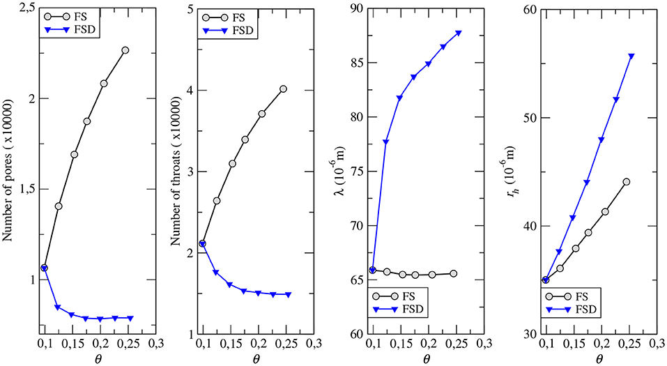
Figure 2. From left to right: number of pores; number of throats; mean throat length λ; mean throat radius r_h vs. porosity θ for the FS and FSD samples.

A pulse of constant concentration at the sample inlet (z = 0) is applied at t = 0 by locating particles in a flux weighted injection mode. Note that the pulse is formally an exponential distribution function of characteristic time τ_j|_{z = 0} whose mean value is negligible compared to the mean time required for the particles to move through the sample (Russian et al., 2016). Flux weighted injection means that the number of particles injected at a location is proportional to the local velocity. This corresponds to a constant concentration Dirichlet boundary condition. Particles that reach the sample outlet with a speed v_out are reinjected randomly at the inlet plane at a position x satisfying the condition |v_x−v_out|≪〈v〉.

The distribution (PDF) of first passage times at a given distance Z from the injection location, that denotes the solute breakthrough curve (BTC) usually measured in laboratory or field tracer tests, is noted f_t(t) (Figure 8). The apparent longitudinal dispersion coefficient D(t) is evaluated from the displacement variance ${\sigma }_z^2(t)$ of the particles (Fischer, 1966):

$\begin{array}{ll}D(t)=\frac{1}{2}\frac{d{\sigma }_z^2(t)}{dt},& (9)\end{array}$

with ${\sigma }_z^2(t)=\langle {(z(t)-\langle z\rangle )}^2\rangle -{\langle z(t)-\langle z\rangle \rangle }^2$. The asymptotic longitudinal dispersion coefficient $D^{*}={\sigma }_z^2(t)/2t$ is obtained for t>t^*, where t^* is the time required for all the particles to sample the entire heterogeneity, i.e., when ${\sigma }_z^2(t)~t$ (see for example Figure 10).

2.4. The Equivalent Bond Network Model

We compute the bond network model (BNM) for each of the FS and FSD samples in order to extract the geometrical and topological characteristics of the connected porosity. The methodology to obtain the network representation of the connected porosity of the sample includes two main steps. The first one is the extraction of the void space skeleton which is the one-dimensional continuous object centrally located (and spatially referenced) inside the pore space. The skeleton can be computed using different approaches; here we used a thinning algorithm inspirited from the works of Lee et al. (1994) that provides the local medial-axis. The coordinate of the skeleton is known with a spatial resolution equivalent to that of the original 3D-image and associated with the local hydraulic radius r_l normal to the local medial axis that is evaluated using a pondered 45 degree multi-ray method. Thus, the skeleton keeps the relevant geometrical and topological features of the pore space (Siddiqi and Pizer, 2008). The second step consists in transforming the skeleton into a network of bonds and nodes that connect three or more bonds. This yields an irregular lattice. The length λ of a given bond is the sum of the length of the skeleton components used to built this bond, so that the local tortuosity of the skeleton is embedded into λ. For each bond, the radius r_h is obtained from the harmonic means (noted 〈〉_H) of the local conductance, so that $r_h={({\langle r_l\rangle }_H)}^{1/4}$. The algorithm is non-parametric; there is no assumption on any of the characteristics of the obtained lattice.

2.5. Upscaled CTRW Model

The central assumption of this model is that transition times at subsequent CTRW steps are independent identically distributed random variables. Furthermore, it is assumed that particles move at the mean pore velocity, that is, it is assumed that during a transition particles are able to diffusively sample the velocities across pore conducts. The scale ℓ_c is set equal to the decorrelation distance of particle speeds so that subsequent particle speeds can be considered statistically independent. The distribution of the Eulerian mean flow speeds p_m(v) is obtained from the Eulerian speed PDF as

$\begin{array}{ll}{p}_m(v)=-2v\frac{d{p}_e(2v)}{dv}.& (10)\end{array}$

As particles move at equidistant spatial steps, they sample flow speeds in a flux-weighted manner. This is due to the fact that particles are distributed at pore intersections according to the relative downstream fluxes. Thus, the distribution p_v(v) of subsequent particle speeds are related to the distribution of Eulerian mean flow speeds through flux-weighting as (Puyguiraud et al., 2021).

$\begin{array}{ll}{p}_v(v)=\frac{v{p}_m(v)}{\langle v_m\rangle }.& (11)\end{array}$

At each turning point of the CTRW, particles are assigned a random speed from p_v(v). The particle transition time distribution ψ(t) reflects both advection and diffusion. It is cut-off at times larger than ${\tau }_D={\ell }_c^2/d_m$, the diffusion time over the decorrelation distance. For times small compared to the cut-off time, ψ(t) can be approximated by

$\begin{array}{ll}\psi (t)=\frac{{\ell }_c^2}{t^3\langle v_m\rangle }{p}_m({\ell }_c/t).& (12)\end{array}$

At times larger than τ_D it is cut-off exponentially fast.

The flow speed distribution is at the center of the transport process. In porous media, such as rocks, the mean flow speed can often be approximated by a Gamma-type distribution (Dentz et al., 2018; Puyguiraud et al., 2019b; Souzy et al., 2020) and displays a power-law scaling $p_e(v)~v^{\alpha -1}$ for v < 〈v_m〉. For sphere packs and simple structures such as sand-pack the linear flow profile close to the grains (due to the no-slip boundary condition) implies that p_e(v) is flat at low velocities, so that α≃1 (Dentz et al., 2018). In more heterogeneous porous media, other values of α are expected. For example, Puyguiraud et al. (2021) found α≈0.35 for a Berea sandstone sample. For such Gamma-type distributions, $p_e(v)~v^{\alpha -1}$ at small flow speeds, ψ(t) behaves for high Péclet numbers as ψ(t)~t^−2−α before the exponential cut-off at times larger than τ_D. The tortuosity of particle trajectories in this framework is given by the ratio of the mean asymptotic particle speed ℓ_c/〈τ〉≡〈v_e〉 (where 〈τ〉 denotes the particle mean travel time) and the mean streamwise flow velocity 〈v_z〉. Furthermore, for this type of flow speed distributions, the CTRW approach predicts some further interesting scaling laws that can be verified from direct numerical simulations. The behavior of particle breakthrough curves f(t, Z) at a control plane located at the streamwise location Z is analogous to the behavior of ψ(t). They show a power-law dependence as f(t, Z)~t^−2−α if Z/v_z≪τ_D (i.e., the peak time is much smaller than the cut-off time), and exponential decay for times larger than the cut-off time τ_D. The predicted dependence of the asymptotic longitudinal dispersion coefficients on the Péclet number is for Pe≫1

$\begin{array}{ll}\frac{D^{*}}{d_m}~P{e}^{2-\alpha }& (13)\end{array}$

for 0 < α <1 and

$\begin{array}{ll}\frac{D^{*}}{d_m}~PelnPe& (14)\end{array}$

for α = 1, see also Saffman (1959) and Koch and Brady (1985).

To sum-up, this upscaled model, constructed on the representation of the hydrodynamic transport as a CTRW process in a 1-dimensional network of bonds, is fully constrained, for any values of Pe>1 by the knowledge of the distribution of Eulerian flow speeds p_e(v) and the decorrelation distance ℓ_c of particle speeds.

From here one can recognize on one hand the complementarity of the BNM and the DNS to explore the relation between the dispersion and the pore network characteristics, and on the other hand the conceptual framework that links the CTRW model and the BNM representation of the porous medium. This emphasizes the possibility of (1) relating the distribution of the Eulerian flow speed to the large scale transport behavior and (2) characterizing dispersion for different porous media based on the knowledge of the flow speed distribution. Indeed, the BNM gives us the information on the real topology of the pore network as well as the distribution and the average of bond properties (radius and length), while the DNS provides the information on the flow field (speed distribution and decorrelation distance as well as the advective tortuosity).

3. Pore Network Properties, Flow Fields, and Dispersion

The top row in Figure 1 illustrates the 3-dimensional structure of sample FS10 (θ = 0.1) and of both FS25 and FSD25 sharing the same porosity θ = 0.25. The bottom row in Figure 1 displays flow lines (and the local velocity) within the connected porosity for these three samples and gives a qualitative appraisal of the dissimilarities between the lowest porosity and the highest porosity samples on one hand, and on the other hand those occurring between the highest porosity sample of each of the two sets in relation with the pore network structures. In the following we will quantify these differences and their implications on dispersion.

3.1. Connected Porosity Geometrical Properties Retrieved From the BNM

As explained in section 2.1, we computed the Bond Network Model (BNM) for each of the 12 samples, in order to evaluated the topology and the geometry of the connected porosity and specifically how these characteristics change with the sample porosity for the FS and the FSD sets of samples. The main properties vs. porosity are summarized in Figures 2, 3. The topology of the connected porosity is characterized by the number of throats (network bonds) and pores (network nodes) per volume of rock (here the reference is the sample volume) as well as the coordination number κ that denotes the mean number of throats connected to a given pore. The bonds are characterized by the mean of the radius r_h and length λ and by the radius r_h distribution displayed in Figure 4.

FIGURE 3

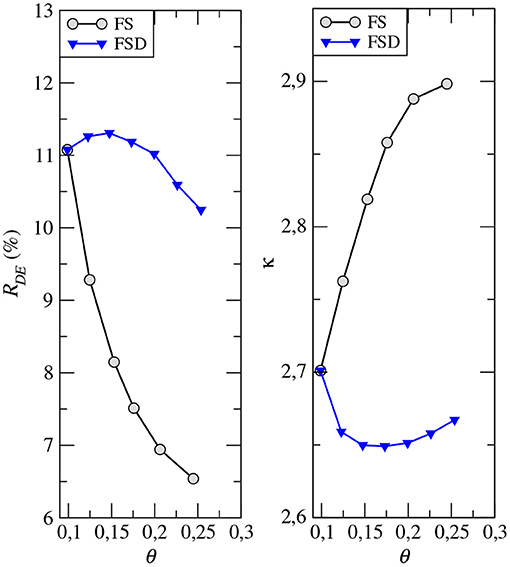
Figure 3. Left: Ratio (in %) of the number of dead-ends to the number of throats. Right: Mean number of throats per pore κ vs. porosity θ for the FS and FSD samples.

FIGURE 4

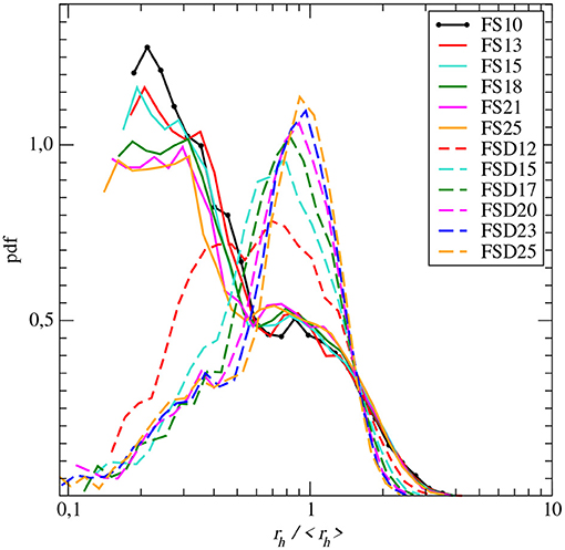
Figure 4. Normalized distribution of r_h for the FS and FSD samples.

For the FS set, decreasing porosity from the highest to the lowest porosity values is obtained by allocating increasing amounts of cement into localized clusters that acts as increasingly closing connections and thus decreasing the number of pores and throats and the coordination number. The fixed distribution of the cement clusters determines the length of the bonds independently of the porosity (λ≈65μm), but volume conservation imposes that the hydraulic radius r_h increases with porosity. The distribution of r_h/〈r_h〉 is wide, decreases almost monotonically from small to high r_h and does not depends on porosity.

For the FSD set, increasing porosity from the lowest to the highest is obtained by homogeneous erosion of the solid phase, i.e., both the grains and the cement. The number of pores and throats as well as κ first decreases for θ ≤ 0.15 caused by merging of adjacent throats following a process which is roughly the opposite of that described for the FS set of samples. Then, the number of pores and throats stays almost constant for θ>0.15. As a result, the increase of porosity is mainly due to the increase of the throat length λ and radius r_h. The distribution of r_h/〈r_h〉 is almost Gaussian around the mean value, and independent of the porosity for θ>0.15. The transition from the original sample FS10 to the FSD12 and then FSD15 is well visible the r_h distribution. Note that, as soon as the throats are widely distributed like for the FS set of samples, κ is an indicator of the potential local flow rate disorder at the network nodes because the probability of having upstream and downstream bonds of distinctly different flow rates is high.

Altogether, these results show that the two sets of samples are very different in terms of (1) the topology of the network; for the FSD set, the topology is almost similar for all the porosity range, while it is increasingly complex (with increasing tortuosity, see discussion below) as porosity decreases for the FS set of samples, and (2) the characteristic size of the throats which is almost independent of the porosity for the FD set whereas it increases with porosity for the FSD set.

3.2. Permeability and Flow Field Properties

Permeability values k for the 12 samples computed using Darcy's law ($k={\overline{v}}_z\mu /{\nabla }^{*}p$) are plotted in the left panel of Figure 5. Permeability increases from 1.4 × 10⁻¹³m² for sample SF10 to 6.04 × 10⁻¹²m² (6.08 × 10⁻¹²m²) for sample SF25 (SFD25) and are all aligned with the relation k~θ⁴ independently on geometrical characteristics of the pore space. The permeability computed on the BNM (solving a Kirchhoff problem) is also reported Figure 5 in order to evaluate the accuracy of the BNM.

FIGURE 5

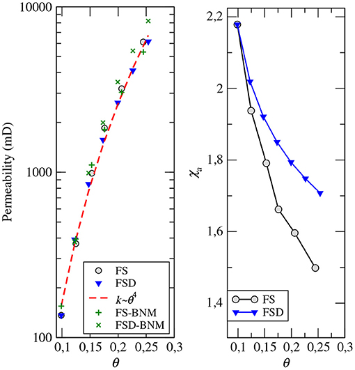
Figure 5. Permeability (left) and advective tortuosity χ_a (right) vs. porosity θ for the FS and FSD samples.

The right panel of Figure 5 displays the advective tortuosity χ_a, i.e., the mean tortuosity of the flow lines. The advective tortuosity is obtained from the ratio of the mean Eulerian speed v_e to the mean velocity in the direction of the flow v_z (Koponen et al., 1996; Ghanbarian et al., 2014; Puyguiraud et al., 2019c): χ_a = 〈v_e〉/〈v_z〉. For both the sets of samples, χ_a decreases when porosity increases, but it is more pronounced for the FS set of samples. These trends seem to be mainly controlled by the increase of the throat radius as porosity increases, while the topological characteristic of the network plays a minor role which is probably resulting from a complex coupling of the geometrical and topologically parameters discussed above. This makes the advective tortuosity, which is one of the three parameters of the CTRW model proposed by Puyguiraud et al. (2021), an intrinsic characteristic of the hydrodynamic system that is essentially porosity-dependant.

The distributions of the Eulerian mean speed for the 12 samples are plotted in Figure 6. The dissimilarity of the p_m(v) curves between the FS and the FSD sets is clearly visible. The FSD samples are displaying almost the same mean speed distributions with power-law trend $p_m(v)~v^{\alpha -1}$ for v < 〈v_m〉 with α = 0.245±0.05. For the FS set, the evolution of p_m(v) with porosity includes two features. First, p_m(v) gradually diverges from a Gamma distribution as porosity increases, with the occurrence of increasingly marked transition between the values of speed larger than the mean (v>〈v_m〉) and the power-law slope for the slower speed values. Second, the power-law slope for v≪〈v_m〉 increases when porosity decreases, ranging from β = α−1 = 1.63 for θ = 0.25 to β = 1.75 for θ = 0.10. These values are in agreement with the value of 1.65 found by Puyguiraud et al. (2021) for the Beara sandstone. As far as we know, they have been very few studies of the correlation between the flow speed distribution and the properties of the pore space microstructures (Siena et al., 2014; Matyka et al., 2016; Alim et al., 2017). For instance, Alim et al. (2017) investigated this issue using numerical simulations in 2-dimensional simple artificial porous media made of circular or elliptical discs placed on a square or triangular lattices with increasing disorder. By extracting and analyzing the corresponding network of tubes, following a procedure quite similar to that implemented for extracting the BNM (section 2.4), they concluded that the flow distribution is mainly determined by the distribution of fractions of fluid flowing at each of the network node and not by the overall tube size distribution. Our results lead us to a similar conclusion for the complex 3-dimensional porous media studied here. The evolution of the mean flow speed with porosity for the FS set in comparison with the weak evolution of the mean flow speed with porosity for the FSD set appears to be correlated to the noticeable increase with porosity of the number of throats as well as the mean number of throats per pore κ (Figure 3) measured for the FS set, whereas both the number of throats and κ are almost constant for the FSD set of samples.

FIGURE 6

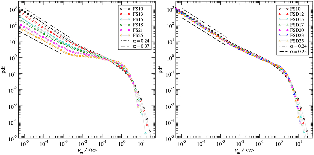
Figure 6. Distribution of the Eulerian mean speeds p_m(v) normalized to its mean, for the FS (left) and the FSD (right) samples.

3.3. Speed Decorrelation Distance Length

The decorrelation distance ℓ_c is evaluated from the Lagrangian flux weighted speed autocorrelation function ${{\rm Y}}_{vv}(l)=\langle (v_v(s)-\langle v_v\rangle )(v_v(s+l)-\langle v_v\rangle )\rangle /{\sigma }_{v_v}^2$, where l denotes the lag. The decorrelation distance ℓ_c is given by the value of the lag corresponding to Υ_vv(l) = 1/e. The two panels at left of Figure 7 display the Lagrangian flux weighted speed autocorrelation function Υ_vv(l) for the two set of samples. The corresponding values of the decorrelation distance ℓ_c vs. porosity are given in the third panel of Figure 7, and the ratio of the decorrelation distance to the mean throat length η = ℓ_c/λ vs. porosity is given in the right panel.

FIGURE 7

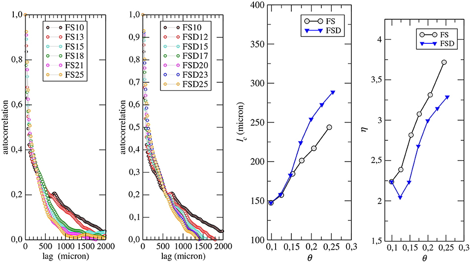
Figure 7. Flux weighted Langrangian speed auto-correlation function Υ_vv(l) for the FS (left) and the FSD (middle-left) samples. The middle-right panel displays the decorrelation length ℓ_c and the right panel displays the ratio η = ℓ_c/λ vs. porosity.

For both the sample sets, the decorrelation distance ℓ_c increases with porosity from about 150 μm at θ = 0.1 to about 240 μm for FS and 290 μm for FSD. The slight increase of ℓ_c for the FSD set for θ>0.15 compared to the FS set is caused by the increase of the throat radius and the decrease of tortuosity with porosity that are more important for FSD than for FS. The ratio η also displays an increase with porosity following a similar trend for both the FS and the FSD set of samples, the values for FSD being smaller of ~0.5 unit than for FS. Thus, in average, the number of bond lengths traveled before losing the memory of the initial speed ranges from about 2 to 4. These values are in good agreement with the value of 4 obtained by Puyguiraud et al. (2021) by fitting DNS and CTRW for Berea sandstone of porosity 0.18.

3.4. Dispersion

In this section, we are presenting the results of the transport DNS, discussing them in the frame of the scaling properties derived from the CTRW model proposed by Puyguiraud et al. (2021) and of the properties retrieved from the BNM (section 3.1).

The first passage time distributions f_t(t) (or breakthrough curves) at a distance of 20 times the sample size are given in Figure 8 for Pe = 100 and also for purely advective transport (d_m = 0;Pe = ∞). For the latter, all the curves display the power-law tailing that characterize pre-asymptotic (non-Fickian) regime over 3 to 4 orders of magnitude. The scaling $f_t(t)~t^{-2-\alpha }$ predicted by Puyguiraud et al. (2021) with the values of α corresponding to those measured on the mean speed distribution is confirmed for all the samples. The comparison of the value of α (0.24 ≤ α ≤ 0.37) for the FS set of samples is given in Figure 9. For Pe = 100, even if it can be considered a quite large value for natural porous media, diffusion acts as increasing the rate at which f_t(t) decreases with time and the α-dependent power-law trend is not present. Note that the beginning of the exponential decrease is visible for FSD25 at t≈5τ_D, where ${\tau }_D={\ell }_c^2/d_m\approx 80s$.

FIGURE 8

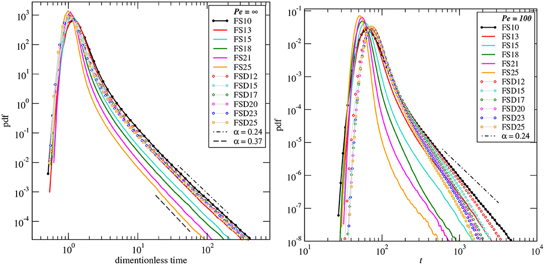
Figure 8. First passage time PDF f_t at Z = 5.47 × 10⁻²m from the inlet. Left: results for infinite Pe vs. dimensionless time Z/v. Right: results for Pe = 100 vs. time.

FIGURE 9

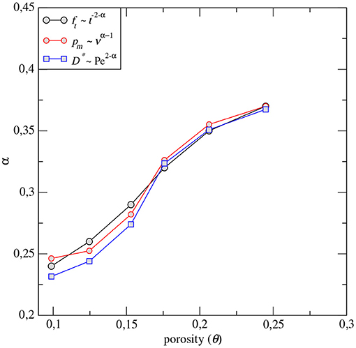
Figure 9. Comparison of the value of α for the FS samples evaluated from (1) the slope of the first passage time plotted in the left panel, (2) the slope of the mean speed PDF plotted in Figure 6 and (3) the slope of the $D^{*}/d_m$ vs. Pe plotted in Figure 11.

We now focus on determining the asymptotic dispersion coefficient D^* from the asymptotic regime of the displacement variance. Figure 10 displays, as an example, the displacement variance normalized to the throat length (σ²/λ²) for the 12 samples in the case Pe = 100, but the following comments apply for all values of Pe larger than 1. All curves converge to the asymptotic regime (σ²/λ²~t) for time t≥t_a, where t_a is independent of the value of Pe but depends on porosity; $t_a\approx 10^3$s for θ = 0.1 and $t_a\approx 10^4$s for θ = 0.25, i.e., about 40 and 120 times τ_D, respectively. This point is important regarding the possibilities of measuring the asymptotic dispersion from laboratory experiments, deriving D^* from the breakthrough curves, for instance. For Pe = 100, that corresponds to a mean flow speed of 1.5 × 10⁻³ m/s for FS10, a sample of about 1.5 m long displaying the same properties of the mm-scale sample would be necessary to measure D^*; a distance of 60 m would be necessary for Pe = 4,000. This indicates that experimental measurement of D^* can be performed only for low values of Pe, typically of the order Pe ≤ 10. However, for such low values of Pe it is not possible to measure α and thus determine the trend D^*(Pe).

FIGURE 10

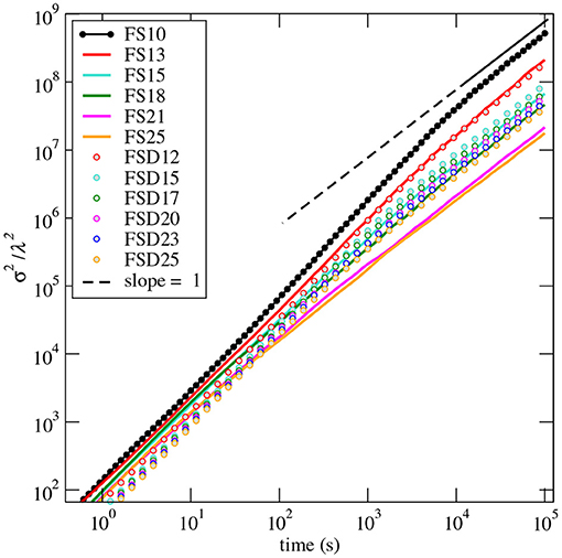
Figure 10. Normalized z-direction displacement variance vs. time for Pe = 100.

Conversely, the DNS allows us to perform numerical experiments over large range of Pe values; Figure 11 displays the value of D^* vs. Pe for the 12 samples from diffusion-dominant regime (Pe = 10⁻³) to advection-dominant (Pe = 2 × 10⁴). These curves can be commented in terms of their slope and of their scaling with porosity, for Pe≫1. Note that for Pe → 0 the ratio $D^{*}/d_m$ is equal to the inverse of the diffusive tortuosity ($D^{*}/d_m={\chi }_d^{-1}$). For both the FS and FSD sets of samples, the relation $D^{*}/d_m\propto P{e}^{2-\alpha }$ predicted by the CTRW model for Pe≫1 is observed. The values of α compared to those measured using the speed distribution and the tailing of f_t(t) are given in Figure 9. The minimum value Pe_c at which $D^{*}/d_m\propto P{e}^{2-\alpha }$ is effectively observed, is correlated with the shape of the mean speed distribution (Figure 6). For FS10, the trend $p_m(v)~v^{\alpha -1}$ with α = 0.24 extends up to $5\times 10^{-3}v/\langle v_m\rangle$, while for FS25 the trend α = 0.37 extends up to $3\times 10^{-4}v/\langle v_m\rangle$ only. This gives values of Pe_c ranging from 1,000 for FS10 to 50 for FS25. The same trend is observed for the FSD set of samples. These results demonstrate the clear control of the particle mean speed distribution on the evolution of D^* with the Péclet number. However, both the two sets of samples display a scaling of D^* with porosity, independently of the slope determined for Pe≥Pe_c. The expected decrease of D^* for all values of Pe>1 when porosity increases, corresponding to a decrease of the slope of p_m(v) for v≪〈v_m〉 is clearly visible for the FS set of samples. But, the results for the FSD set, that share the same mean speed distribution (Figure 6), show also a clear decrease of D^* as porosity increases, which indicates that the dispersion scaling with porosity is not solely controlled by p_m(v) for v≪〈v_m〉. Indeed, the increase of D^* with porosity is also related to the increase of the speed decorrelation distance ℓ_c with porosity. In the frame of the CTRW model l_c denotes the length at which a new velocity is drawn from the mean speed distribution, and as such ℓ_c determines the rate at which the speed changes.

FIGURE 11

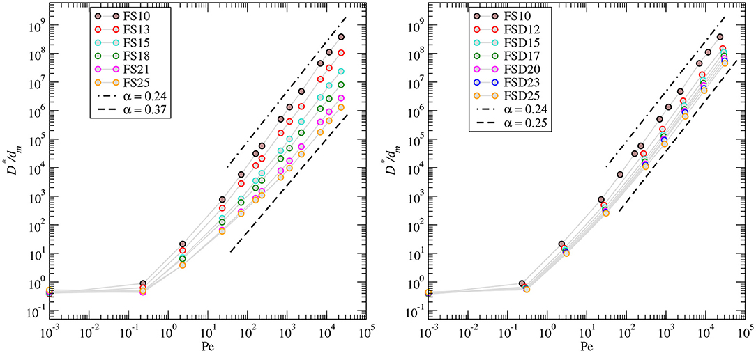
Figure 11. Asymptotic dispersion coefficient vs. Pe for the FS and FSD samples.

Furthermore, we observe in Figure 11 that D^* shows different power-law behaviors for Pe < Pe_c that can be related to the scaling behavior of the distribution of mean flow speeds and the transition time distribution. In the limit of infinite Pe, the transition time distribution is given by (Equation 12). For finite Pe, it is cut-off at the diffusion time τ_D. The log-slope of ψ(t) at the cut-off time depends on the average flow speed 〈v_m〉. This is shown in Figure 12, which displays the distribution of purely advective transition times rescaled by τ_v = ℓ_c/〈v_m〉 for FS10 and FS25. The behavior of D^* for Pe < Pe_c corresponds to the power-law scaling of ψ(t) at dimensionless times equal to Pe. The slope of the ψ(t) curves display the power-law behaviors t^−2−α′ for Pe < Pe_c with α′ = 0.38 and 0.79 for FS10 and FS25, respectively. For Pe≥Pe_c the values of α are similar to those reported in Figure 9 for f_t(t), p_m(v) and D^*(Pe), i.e., α = 0.23 and 0.37 for FS10 and FS25, respectively.

FIGURE 12

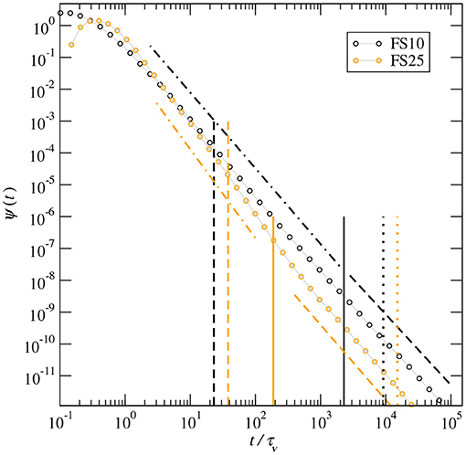
Figure 12. Distribution of advective transition times rescaled by τ_v for FS10 and FS25. The dimensionless cut-off time is Pe = τ_D/τ_v. The vertical lines denote Pe = 10 (dashed lines), Pe = Pe_c (solid lines) and Pe= 4,000 (dot line). The sloped lines denote the power-law behaviors t^−2−α′ for Pe < Pe_c with α′ = 0.38 and 0.79 for FS10 and FS25, respectively, and t^−2−α for Pe≥Pe_c with α = 0.23 and 0.37 for FS10 and FS25, respectively.

4. Summary and Conclusions

We performed numerical experiments of passive solute transport for two sets of porous media mimicking a large range of porosity and microstructures expected in sandstones. The aim was to test the validity of the CTRW model, to explore how the flow field characteristics are linked to the porous media geometrical properties and to determine the scaling of asymptotic dispersion coefficient D^* with the Péclet number. The two sets of six samples share similar porosity, ranging from 0.1 to 0.25, and the same permeability-porosity trend k(θ) but displays distinctly different microstructures and thus dispersion evolution.

The conceptual CTRW model of solute transport in porous media, as the one proposed by Puyguiraud et al. (2021), infers that solute spreading along particle paths is controlled by the transition time of the solute particles which is determined by the distribution of solute particle mean speeds p_m(v), the velocity decorrelation distance ℓ_c and diffusion. The effective tortuosity factor that depends on Pe and on the advective tortuosity χ_a (that can be also easily evaluated form the flow field) allows mapping dispersion in the streamwise direction which is aligned with the mean pressure gradient. With decreasing Pe, the effective tortuosity of the solute particles increases and the control of p_m(v) on dispersion decreases but remains important up to high values of Pe because of the wide distribution of the particles speeds toward low speed values. This means that for heterogeneous media, such as sandstones, the pre-asymptotic (non-Fickian) dispersion regime is likely to persist over long time scales.

We found that the scaling properties, measured by the coefficient α, predicted by Puyguiraud et al. (2021)'s model are effectively measurable for all the 12 studied samples. For instance, results shows that at high Pe, the tail of the breakthrough curves, that is controlled by the low flow speeds, scales as $f_t(t)~t^{-2-\alpha }$ where α is given by the slope of the mean speed distribution $p_m(v)~v^{\alpha -1}$, for v < 〈v_m〉. As Pe decreases, diffusion eventually dominates over low flow speeds, thus cuts off the power-law tail of the breakthrough curves and leads to Fickian behavior from which the asymptotic dispersion coefficient D^* can be theoretically evaluated (Van Genuchten and Wierenga, 1986). However, the analysis of the displacement variance σ²(t) indicates that D^* cannot be measured experimentally at laboratory scale, for high values of Pe, because the distance required for reaching the asymptotic regime is orders of magnitude larger than what is workable at laboratory scale. Thus, measuring experimentally the value of α, for determining how D^* scales with Pe seems difficult.

The asymptotic dispersion coefficient D^* was computed up to the largest values of Pe expected for laminar flow in natural environments. Results show that $D^{*}/d_m\propto P{e}^{2-\alpha }$ from Pe_c up to the highest value of Pe (Pe= 4,000). Note that for the values of α expected for such heterogeneous rock samples, neither the trend D^*~Peln(Pe) (Saffman, 1959; Koch and Brady, 1985) assuming that the distribution of flow speeds is flat (α = 1), nor the trend D^*~Pe expected for α>1 at high Pe are expected. For 1 < Pe < Pe_c, $D^{*}/d_m\propto P{e}^{2-{\alpha }^{\prime }}$ where α′>α depends on the mean speed distribution and the speed decorrelation distance ℓ_c that are the parameters that determine the advective particle transition distribution and subsequently the value of Pe_c. The mean particle speed remains correlated for longer distances in porous media with straighter and larger bonds (throats). As such ℓ_c is a good indicator of the complexity of flow field, because it encompasses the effect of tortuosity that ubiquitously decreases with increasing porosity and the effect of the mean throat radius that ubiquitously increases with porosity, while the other structural parameters are distinctly different for the two sets of samples. Yet, when reported in term of number of bonds length traveled before speed decorrelates, it is observed that FS and FSD sets behave quite similarly; the equivalent number of pores (intersection nodes) crossed before losing the memory of the initial speed equals η−1 and ranges from about 1 for θ = 0.1 to about 3 for θ = 0.25. We conjecture that the increase of the number nodes crossed before speed decorrelates is linked to the speed changes caused by the splitting of the flow at the network node and thus to both the mean radius of the bonds and the coordination number κ. Similar conjecture can be done for the distribution of the solute mean speed p_m(v) which should be controlled by the speed changes caused by splitting of the flow where throats are connected, as it was anticipated by Alim et al. (2017) in numerical simulations in 2-dimensional simple artificial networks. The structural and hydrodynamic mechanisms that determine the flow distribution in 3-dimensional porous media, focusing on the impact pore size distribution, coordination number and local correlations on the speed distributions will be discussed in a forthcoming paper. Yet, from the results presented in this paper, one can conclude that the flow distribution, and thus the mean speed, are controlled by the distribution of fractions of fluid flowing at each of the network nodes which in turn is determined by the distribution of the throat radius (and not the mean) and the coordination number. At given porosity and mean bond radius the latter is controlled by the number of throats per unit volume that increases with porosity for the FS set and decrease with porosity for the FSD set of samples. We believe that these results give a first insight into both the mechanisms and the microstructural parameters that control dispersion in porous media.

Data Availability Statement

The original contributions presented in the study are included in the article/supplementary material, further inquiries can be directed to the corresponding author/s.

Author Contributions

All authors contribute to all the aspects of the presented work.

Conflict of Interest

The authors declare that the research was conducted in the absence of any commercial or financial relationships that could be construed as a potential conflict of interest.

Publisher's Note

All claims expressed in this article are solely those of the authors and do not necessarily represent those of their affiliated organizations, or those of the publisher, the editors and the reviewers. Any product that may be evaluated in this article, or claim that may be made by its manufacturer, is not guaranteed or endorsed by the publisher.

Acknowledgments

The authors gratefully acknowledge the support of the CNRS-PICS project CROSSCALE (Project No. 280090). A. P. and M. D. gratefully acknowledge the support of the Spanish Ministry of Science and Innovation through the project HydroPore (PID2019106887 GB-C31). Computations have been realized with the support of MESOLR, the Center of Competence in High-Performance Computing from the Languedoc-Roussillon region, France.

References

Alim, K., Parsa, S., Weitz, D. A., and Brenner, M. P. (2017). Local pore size correlations determine flow distributions in porous media. Phys. Rev. Lett. 119:144501. doi: 10.1103/PhysRevLett.119.144501

PubMed Abstract | CrossRef Full Text | Google Scholar

Bear, J. (1972). Dynamics of Fluids in Porous Media. New York, NY: American Elsevier.

Google Scholar

Berg, C. F. (2016a). Fontainebleau 3d Models. Available online at: http://www.digitalrocksportal.org/projects/57

Google Scholar

Berg, C. F. (2016b). Fundamental transport property relations in porous media incorporating detailed pore structure description. Transport Porous Media 112, 467–487. doi: 10.1007/s11242-016-0661-7

CrossRef Full Text | Google Scholar

Bijeljic, B., and Blunt, M. J. (2006). Pore-scale modeling and continuous time random walk analysis of dispersion in porous media. Water Resour. Res. 42:W01202. doi: 10.1029/2005WR004578

CrossRef Full Text | Google Scholar

Bijeljic, B., and Blunt, M. J. (2007). Pore-scale modeling of transverse dispersion in porous media. Water Resour. Res. 43:W12S11. doi: 10.1029/2006WR005700

CrossRef Full Text | Google Scholar

Bijeljic, B., Mostaghimi, P., and Blunt, M. J. (2011). Signature of non-Fickian solute transport in complex heterogeneous porous media. Phys. Rev. Lett. 107:204502. doi: 10.1103/PhysRevLett.107.204502

PubMed Abstract | CrossRef Full Text | Google Scholar

Bijeljic, B., Muggeridge, A. H., and Blunt, M. J. (2004). Pore-scale modeling of longitudinal dispersion. Water Resour. Res. 40:W11501. doi: 10.1029/2004WR003567

PubMed Abstract | CrossRef Full Text | Google Scholar

Bijeljic, B., Raeini, A., Mostaghimi, P., and Blunt, M. J. (2013). Predictions of non-fickian solute transport in different classes of porous media using direct simulation on pore-scale images. Phys. Rev. E 87:013011. doi: 10.1103/PhysRevE.87.013011

PubMed Abstract | CrossRef Full Text | Google Scholar

Brenner, H., and Edwards, D. (1993). Macrotransport Processes. Boston: Butterworth-Heinemann, MA.

Google Scholar

Carrel, M., Morales, V. L., Dentz, M., Derlon, N., Morgenroth, E., and Holzner, M. (2018). Pore-scale hydrodynamics in a progressively bioclogged three-dimensional porous medium: 3-d particle tracking experiments and stochastic transport modeling. Water Resour. Res. 54, 2183–2198. doi: 10.1002/2017WR021726

PubMed Abstract | CrossRef Full Text | Google Scholar

Chatzis, I., and Dullien, F. A. (1985). The modeling of mercury porosimetry and the relative permeability of mercury in sandstones using percolation theory. Int. Chem. Eng. 25:1.

Google Scholar

Danckwerts, P. (1953). Continuous flow systems: distribution of residence times. Chem. Eng. Sci. 2, 1–13. doi: 10.1016/0009-2509(53)80001-1

CrossRef Full Text | Google Scholar

De Anna, P., Le Borgne, T., Dentz, M., Tartakovsky, A. M., Bolster, D., and Davy, P. (2013). Flow intermittency, dispersion, and correlated continuous time random walks in porous media. Phys. Rev. Lett. 110:184502. doi: 10.1103/PhysRevLett.110.184502

PubMed Abstract | CrossRef Full Text | Google Scholar

Delay, F., Ackerer, P., and Danquigny, C. (2005). Simulating solute transport in porous or fractured formations using random walk particle tracking. Vadose Zone J. 4, 360–379. doi: 10.2136/vzj2004.0125

CrossRef Full Text | Google Scholar

Delgado, J. M. P. Q. (2006). A critical review of dispersion in packed beds. Heat Mass Transfer 42, 279–310. doi: 10.1007/s00231-005-0019-0

CrossRef Full Text | Google Scholar

Dentz, M. (2012). Concentration statistics for transport in heterogeneous media due to stochastic fluctuations of the center of mass velocity. Adv. Water Resour. 36, 11–22. doi: 10.1016/j.advwatres.2011.04.005

CrossRef Full Text | Google Scholar

Dentz, M., Borgne, T. L., Englert, A., and Bijeljic, B. (2011). Mixing, spreading and reaction in heterogeneous media: a brief review. J. Contaminant Hydrol. 120–121:1–17. doi: 10.1016/j.jconhyd.2010.05.002

PubMed Abstract | CrossRef Full Text | Google Scholar

Dentz, M., Icardi, M., and Hidalgo, J. J. (2018). Mechanisms of dispersion in a porous medium. J. Fluid Mech. 841, 851–882. doi: 10.1017/jfm.2018.120

PubMed Abstract | CrossRef Full Text | Google Scholar

Fischer, H. B. (1966). Longitudinal Dispersion in Laboratory and Natural Streams. Technical report, California Inst. of Technology.

Google Scholar

Ghanbarian, B., Hunt, A. G., Ewing, R. P., and Skinner, T. E. (2014). Universal scaling of the formation factor in porous media derived by combining percolation and effective medium theories. Geophys. Res. Lett. 41, 3884–3890. doi: 10.1002/2014GL060180

PubMed Abstract | CrossRef Full Text | Google Scholar

Gjetvaj, F., Russian, A., Gouze, P., and Dentz, M. (2015). Dual control of flow field heterogeneity and immobile porosity on non-Fickian transport in Berea sandstone. Water Resour. Res. 51, 8273–8293. doi: 10.1002/2015WR017645

PubMed Abstract | CrossRef Full Text | Google Scholar

Gouze, P., Borgne, T. L., Leprovost, R., Lods, G., Poidras, T., and Pezard, P. (2008). Non-fickian dispersion in porous media: 1. Multiscale measurements using single-well injection withdrawal tracer tests. Water Resour. Res. 44:W06426. doi: 10.1029/2007WR006278

CrossRef Full Text | Google Scholar

Gouze, P., Puyguiraud, A., Roubinet, D., and Dentz, M. (2021). Pore-scale transport in rocks of different complexity modeled by random walk methods. Transport Porous Media 1573–1634. doi: 10.1007/s11242-021-01675-2

CrossRef Full Text | Google Scholar

Guibert, R., Horgue, P., Debenest, G., and Quintard, M. (2016). A comparison of various methods for the numerical evaluation of porous media permeability tensors from pore-scale geometry. Math. Geosci. 48, 329–347. doi: 10.1007/s11004-015-9587-9

CrossRef Full Text | Google Scholar

Han, N.-W., Bhakta, J., and Carbonell, R. G. (1985). Longitudinal and lateral dispersion in packed beds: effect of column length and particle size distribution. AIChE J. 31, 277–288. doi: 10.1002/aic.690310215

PubMed Abstract | CrossRef Full Text | Google Scholar

Icardi, M., Boccardo, G., Marchisio, D. L., Tosco, T., and Sethi, R. (2014). Pore-scale simulation of fluid flow and solute dispersion in three-dimensional porous media. Phys. Rev. E 90:013032. doi: 10.1103/PhysRevE.90.013032

PubMed Abstract | CrossRef Full Text | Google Scholar

Kang, P. K., de Anna, P., Nunes, J. P., Bijeljic, B., Blunt, M. J., and Juanes, R. (2014). Pore-scale intermittent velocity structure underpinning anomalous transport through 3-d porous media. Geophys. Res. Lett. 41, 6184–6190. doi: 10.1002/2014GL061475

PubMed Abstract | CrossRef Full Text | Google Scholar

Kinzel, D. L., and Hill, G. A. (1989). Experimental study of dispersion in a consolidated sandstone. Can. J. Chem. Eng. 67, 39–44. doi: 10.1002/cjce.5450670107

PubMed Abstract | CrossRef Full Text | Google Scholar

Koch, D. L., and Brady, J. F. (1985). Dispersion in fixed beds. J. Fluid Mech. 154, 399–427. doi: 10.1017/S0022112085001598

PubMed Abstract | CrossRef Full Text | Google Scholar

Koponen, A., Kataja, M., and Timonen, J. (1996). Tortuous flow in porous media. Phys. Rev. E 54:406. doi: 10.1103/PhysRevE.54.406

PubMed Abstract | CrossRef Full Text | Google Scholar

Lee, T., Kashyap, R., and Chu, C. (1994). Building skeleton models via 3-d medial surface axis thinning algorithms. CVGIP Graph. Models Image Process. 56, 462–478. doi: 10.1006/cgip.1994.1042

CrossRef Full Text | Google Scholar

Levy, M., and Berkowitz, B. (2003). Measurement and analysis of non-Fickian dispersion in heterogeneous porous media. J. Contaminant Hydrol. 64, 203–226. doi: 10.1016/S0169-7722(02)00204-8

PubMed Abstract | CrossRef Full Text | Google Scholar

Li, M., Qi, T., Bernabé, Y., Zhao, J., Wang, Y., Wang, D., et al. (2018). Simulation of solute transport through heterogeneous networks: analysis using the method of moments and the statistics of local transport characteristics. Sci. Rep. 8:3780. doi: 10.1038/s41598-018-22224-w

PubMed Abstract | CrossRef Full Text | Google Scholar

Matyka, M., Gołembiewski, J., and Koza, Z. (2016). Power-exponential velocity distributions in disordered porous media. Phys. Rev. E 93:013110. doi: 10.1103/PhysRevE.93.013110

PubMed Abstract | CrossRef Full Text | Google Scholar

Morales, V. L., Dentz, M., Willmann, M., and Holzner, M. (2017). Stochastic dynamics of intermittent pore-scale particle motion in three-dimensional porous media: experiments and theory. Geophys. Res. Lett. 44, 9361–9371. doi: 10.1002/2017GL074326

PubMed Abstract | CrossRef Full Text | Google Scholar

Moroni, M., and Cushman, J. H. (2001). Statistical mechanics with three-dimensional particle tracking velocimetry experiments in the study of anomalous dispersion. II. Experiments. Phys. Fluids 13, 81–91. doi: 10.1063/1.1328076

PubMed Abstract | CrossRef Full Text | Google Scholar

Oren, P.-E. (2002). Process based reconstruction of sandstones and prediction of transport properties. Transport Porous Media 46, 311–343. doi: 10.1023/A:1015031122338

CrossRef Full Text | Google Scholar

Pfannkuch, H. O. (1963). Contribution a l'étude des déplacements de fluides miscibles dans un milieux poreux. Rev. Inst. Fr. Petr. 18, 215–270.

Google Scholar

Puyguiraud, A., Gouze, P., and Dentz, M. (2019b). Stochastic dynamics of lagrangian pore-scale velocities in three-dimensional porous media. Water Resour. Res. 55:1196–1217. doi: 10.1029/2018WR023702

CrossRef Full Text | Google Scholar

Puyguiraud, A., Gouze, P., and Dentz, M. (2019c). Upscaling of anomalous pore-scale dispersion. Transport Porous Media 128, 837–855. doi: 10.1007/s11242-019-01273-3

CrossRef Full Text | Google Scholar

Puyguiraud, A., Gouze, P., and Dentz, M. (2020). Is there a representative elementary volume for anomalous dispersion? Transport Porous Media 131, 767–778. doi: 10.1007/s11242-019-01366-z

CrossRef Full Text | Google Scholar

Puyguiraud, A., Gouze, P., and Dentz, M. (2021). Pore-scale mixing and the evolution of hydrodynamic dispersion in porous media. Phys. Rev. Lett. 126:164501. doi: 10.1103/PhysRevLett.126.164501

PubMed Abstract | CrossRef Full Text | Google Scholar

Russian, A., Dentz, M., and Gouze, P. (2016). Time domain random walks for hydrodynamic transport in heterogeneous media. Water Resour. Res. 52, 3309–3323. doi: 10.1002/2015WR018511

PubMed Abstract | CrossRef Full Text | Google Scholar

Saffman, P. G. (1959). A theory of dispersion in a porous medium. J. Fluid Mech. 6, 321–349. doi: 10.1017/S0022112059000672

PubMed Abstract | CrossRef Full Text | Google Scholar

Sahimi, M. (2011). Flow and Transport in Porous Media and Fractured Rock: From Classical Methods to Modern Approaches. John Wiley & Sons. doi: 10.1002/9783527636693

PubMed Abstract | CrossRef Full Text | Google Scholar

Sahimi, M., Hughes, B. D., Scriven, L., and Davis, H. T. (1986). Dispersion in flow through porous media–i. one-phase flow. Chem. Eng. Sci. 41, 2103–2122. doi: 10.1016/0009-2509(86)87128-7

CrossRef Full Text | Google Scholar

Sahimi, M., and Imdakm, A. (1988). The effect of morphological disorder on hydrodynamic dispersion in flow through porous media. J. Phys. A 21, 3833–3870. doi: 10.1088/0305-4470/21/19/019

CrossRef Full Text | Google Scholar

Seymour, J. D., and Callaghan, P. T. (1997). Generalized approach to NMR analysis of flow and dispersion in porous media. AIChE J. 43, 2096–2111. doi: 10.1002/aic.690430817

PubMed Abstract | CrossRef Full Text | Google Scholar

Seymour, J. D., Gage, J. P., Codd, S. L., and Gerlach, R. (2004). Anomalous fluid transport in porous media induced by biofilm growth. Phys. Rev. Lett. 93:198103. doi: 10.1103/PhysRevLett.93.198103

PubMed Abstract | CrossRef Full Text | Google Scholar

Siddiqi, K., and Pizer, S. (2008). Medial Representations: Mathematics, Algorithms and Applications, 1st Edn. Springer Publishing Company. doi: 10.1007/978-1-4020-8658-8

CrossRef Full Text | Google Scholar

Siena, M., Riva, M., Hyman, J. D., Winter, C. L., and Guadagnini, A. (2014). Relationship between pore size and velocity probability distributions in stochastically generated porous media. Phys. Rev. E 89:013018. doi: 10.1103/PhysRevE.89.013018

PubMed Abstract | CrossRef Full Text | Google Scholar

Souzy, M., Lhuissier, H., Méheust, Y., Borgne, T. L., and Metzger, B. (2020). Velocity distributions, dispersion and stretching in three-dimensional porous media. J. Fluid Mech. 891:A16. doi: 10.1017/jfm.2020.113

PubMed Abstract | CrossRef Full Text | Google Scholar

Taylor, G. (1953). Dispersion of soluble matter in solvent flowing slowly through a tube. Proc. R. S. Lond. A Math. Phys. Eng. Sci. 219, 186–203. doi: 10.1098/rspa.1953.0139

CrossRef Full Text | Google Scholar

Van Genuchten, M. T., and Wierenga, P. J. (1986). Solute Dispersion Coefficients and Retardation Factors. Madison: John Wiley & Sons, Ltd. doi: 10.2136/sssabookser5.1.2ed.c44

CrossRef Full Text | Google Scholar

Weller, H. G., Tabor, G., Jasak, H., and Fureby, C. (1998). A tensorial approach to computational continuum mechanics using object-oriented techniques. Comput. Phys. 12, 620–631. doi: 10.1063/1.168744

PubMed Abstract | CrossRef Full Text | Google Scholar

Whitaker, S. (1967). Diffusion and dispersion in porous media. AIChE J. 13, 420–427. doi: 10.1002/aic.690130308

PubMed Abstract | CrossRef Full Text | Google Scholar