Optimal investment strategies for decarbonizing the Indian private road transport sector

The Indian government's COP26 emission reduction target has led to explore strategies to decarbonize India's private road transport sector. Adoption of novel vehicle options such as E85, electric, and CNG vehicles and strong network of public transportation are expected to reduce the emissions significantly. A system dynamics model for India's private road transport sector has been developed previously. This study expands that model by incorporating the dynamics between public and private road transportation and uses it to identify strategy for optimal incentive allocation for novel vehicle adoption to minimize the GHG emissions. The idea of epsilon-constraint method for multi objective optimization has been used in this work. The results suggested a trade off between investment in incentives and reduction in GHG emissions. Incentivization strategy prioritized electric cars and two-wheelers, as well as charging/CNG stations, to discourage the adoption of petrol vehicles till CNG infrastructure was established. The minimum GHG emissions achieved was 535.5 Mt CO₂e by 2050 with an investment of 137.74 trillion Indian Rupee when public transportation was not considered. Upon considering public transportation, the minimum GHG emissions further reduced to 464.5 Mt CO₂e by 2050 with reduced investment of 128.25 trillion Indian Rupee, indicating greater emission reduction benefits per unit investment. However, beyond a certain threshold, increase in public transportation resulted in increased incentive investment due to a feedback effect. This necessitates incorporating dynamic analysis into policy strategy. Other strategies such as carbon tax and renewable share in electricity grid proves very effective in reducing GHG emissions as well as incentive investments. However, despite reducing emissions COP26 emission target for 2030 was missed by 34%. Banning the purchase of new petrol and diesel vehicles, along with restrictions on the use of existing petrol and diesel vehicles, could help bridge this gap.

1 Introduction

Decarbonization of the Indian transport sector is essential if India is to achieve its target of becoming a net zero country by 2070. According to Bansal et al. (2021), the transport demand in India has already surged from 1,700 billion pkm (passenger-kilometers) in 2005 to 3,833 billion pkm in 2020. The road transport sector alone accounted for 62.5% of passenger transport demand in 2020 (Kamboj et al., 2022). It was responsible for 87% of the total transport energy demand and 92% of the transport sector's greenhouse gas (GHG) emissions in 2020 (Kamboj et al., 2022). These numbers are projected to rise due to increasing demand for private vehicles, including cars and two-wheelers. The four-wheeler ownership is expected to grow nine-fold, while two-wheeler ownership will reach saturation as income levels rise in the next three decades (Kamboj et al., 2022). Consequently, the passenger modal share of cars and two-wheelers is anticipated to rise from 38% in 2020 to 66% in 2050.

Novel vehicle options, such as E85 [driven on 85% of ethanol in 15% of petrol (gasoline)], electric, and compressed natural gas (CNG) vehicles, are being promoted to reduce carbon intensity of private transport sector. However, their adoption remains very low. In 2022, CNG car sales accounted for 11% of the total sales, up from 5% in 2020, whereas electric and hybrid car sales made up just 2% of total sales in 2022, compared to 0.2% in 2020 (Statista, 2023). Notable obstacles to their mass adoption include higher purchase prices compared to conventional vehicles (Dixit and Singh, 2022; Hema and Venkatarangan, 2022) and lack of sufficient refueling stations (Dwivedi, 2020; Ashok et al., 2022).

The Indian government has been providing financial assistance to encourage the adoption of novel vehicle options through various policies. One notable initiative is the Faster Adoption and Manufacturing of Electric Vehicles (FAME) scheme, which offers INR (Indian Rupees) 15,000/kWh incentives, with a maximum cap of 40% of the electric vehicle's purchase price (Govt of India, 2015). State governments also provide subsidies and tax waivers for electric vehicles while supporting charging infrastructure with capital subsidies, property tax exemptions, and electricity cost coverage during construction (Bureau, 2019). Additionally, the Sustainable Alternative Towards Affordable Transportation (SATAT) scheme provides financial assistance of INR 40 Million per 4,800 kg compressed biogas (CBG) produced per day, with a plant capacity of 12,000 cubic meters CBG per day (IOCL, 2023). The government has allocated funds of INR 1,200 Billion for city gas distribution infrastructure (Ministry of Petroleum and Natural Gas, Government of India, 2023). It also offers subsidies for E85 vehicles, including export subsidies of INR 300 Million for converting surplus sugar into ethanol (The Times Of India, 2021).

Increased use of public transport options such as buses, metros, and local trains is also expected to reduce GHG emissions. This can be due to shared mobility, which takes some vehicles off the road, thereby reducing fuel consumption, or less travel time taken by on-road vehicles due to reduced traffic. The Indian government has recently made substantial investments in the construction and operation of metro lines to address road congestion and reduce transport emissions in Tier I and Tier II cities. The budget allocation for Indian metro rail projects increased from INR 156.3 Billion in 2022–23 to INR 195.2 Billion in 2023–24 (The Economic Times, 2023b). Metro rail is already operational in 16 cities across India, with the Delhi Metro being the largest in terms of the length of the lines. As of November 2023, India boasts 895 kilometers of operational metro lines, facilitating an annual ridership of 2.63 Billion people across the country (World Resources Institute, 2023).

While these incentives and investments are encouraging, ensuring the maximum benefit from these actions is challenging. Several shortcomings of the current approach of deciding incentives can be identified. Firstly, the number of sectors are many, covering a variety of conventional and novel vehicle options. The different vehicle sectors, namely two wheelers and four wheelers, must also be noted here. Secondly, the incentives are decided by different agencies of the government, possibility without taking a holistic view of their interactions. Moreover, since the investments are not one time and instead over a longer time horizon, the time depended structuring of the incentives adds another layer of complexity. The optimum level of incentive may have to be modulated as a function of multiple factors. Finally, the complex underlying dynamics in the transport sector such as the gaps in supply and demand of various fuels such as petrol, diesel, and ethanol, impact of insufficient refueling stations on respective vehicle adoption, cost parity in ICE and EVs, reduction in driving of private vehicles due to strong network of public transportation, and evolving consumer preferences will be affecting the adoption of novel vehicles. The dynamics of the system, combined with the incentivization strategy for novel vehicles, can have either a positive or a negative impact on their adoption, and consequently, on the reduction of GHG emissions in the transport sector. Therefore, it is also important to account for the dynamics of the transport sector to ensure efficient utilization of financial resources. The current strategy for distribution of incentives doesn't lacks a clear plan for how these incentives might be adjusted to respond to the evolving dynamics of the system.

Hence, this study formulates and solves a dynamic optimization model utilizing a system dynamics (SD) model developed by Saraf and Shastri (2023) to determine the optimal incentive strategy for novel vehicle options. First, the system dynamics model developed by Saraf and Shastri (2023) is modified to include the expansion in metro transportation and its impact on usage of private vehicles. The modified system dynamics model is incorporated into the optimization model to identify how the optimal incentive strategy gets affected by inclusion of public transportation.

The key novel contribution of this work is the development of an integrated framework that combines dynamics of the transport sector with the optimization model to determine optimal investment strategies. The results of this analysis provide specific inputs on the relative prioritization of various vehicle options, while capturing their interactions. This has not been reported for the Indian private transport sector. All the studies reported in literature have been done for only some vehicle options, and do not capture aspects such as consumer preferences, environmental performance of the vehicle, fuel price dynamics, impact of lack of infrastructure and related factors on consumer selection. The framework presented here, therefore, will be a valuable decision-making tool for various stakeholders, including the government. Such a framework is not currently available in the Indian context.

The structure of this paper is as follows. Section 2 reviews the literature on the effect of incentives on vehicle adoption. Section 3 briefly summarizes the system dynamics model previously developed. Section 4 describes the optimization problem formulation based on the existing system dynamics model. Section 5 describes the inclusion of metro transportation in the SD model and modifications in the optimization problem. Section 6 presents the results for all the optimization problems and provides insights obtained from the results. The paper concludes with Section 7.

2 Literature review

Several studies have examined the effectiveness of financial incentives in promoting EV adoption in different countries, including Norway (Mersky et al., 2016; Wu and Kontou, 2022), the United States (Jenn et al., 2013), and China (Wu et al., 2021). In a study conducted in the United States, direct purchase rebates were found to significantly increase new battery-operated EV registrations, with approximately 8% increase per thousand dollars of incentive offered (Clinton and Steinberg, 2019). A survey in Greece revealed that 35% of respondents expressed willingness to purchase an electric car if incentives were provided (Mpoi et al., 2023). The authors recommended installing fast chargers, particularly in residential buildings and workplaces. Similarly, a survey conducted in Norway indicated that 84% of battery-operated EV owners considered purchase tax and VAT exemptions crucial for their EV purchase (Bjerkan et al., 2016). A study conducted in Portugal employed market simulations to compare the adoption of EVs with internal combustion engine vehicles, showing that financial incentives effectively promoted EV adoption and led to a 60% reduction in well-to-wheel emissions per kilometer (Santarromana et al., 2020).

Incentive allocation strategy is often modeled as an optimization problem. A nonlinear mixed integer mathematical model was proposed by Wu and Kontou (2022) to optimize the investment allocation between purchase incentive and charging infrastructure investment to induce EV adoption in US market and achieve the emission reduction target. Two vehicle systems were studied, namely, gasoline and electric. Consumer demand for a particular vehicle option was modeled as logistic function considering the purchase and operational cost of vehicle, availability of charging stations, social exposure or word-of-mouth effect of EVs, purchase incentives, etc. The objective function was to minimize the total cost of the vehicle while achieving the emission reduction target. Purchase and infrastructure incentives were the decision variables. Results showed that incentives hit the upper bound during the initial phase of simulation, however as the electric vehicle stocks started to increase on road, social exposure or word-of-mouth effect of EVs led to increased demand for EVs resulting in reduction in incentives. Option of home charging availability and electricity prices significantly affected the incentive trend. Nie et al. (2016) have developed an optimization to optimize the design of incentive policy for electric vehicle adoption in China. Consumer vehicle choice model was developed assuming the consumers' willingness to buy EV would depend on the purchase price of EV, range anxiety, charging station density, and the income of the consumer. The problem minimized the total system cost which was the sum of fuel cost, carbon emission cost, and investment on charging stations. The optimal policy set the investment priority to building charging stations. The result suggested that the charging stations should be built up to the level that allowed full accessibility as soon as possible. In contrast, providing purchase subsidy, which was a widely used policy, did not seem to be cost efficient. A bilevel optimization problem was solved by Falbo et al. (2022) to design optimal public incentive policy to assist consumers using fossil fuel vehicles to switch to electric vehicles. Italian governors have signed an agreement which allows policymakers to temporarily stop the circulation of polluting vehicles (traffic ban) to reduce the PM10 concentration. Policymakers were modeled to minimize the total cost of incentive, hospitalization cost due to increased air pollution and traffic ban cost, while consumer was modeled to minimize the individual cost of vehicle ownership. The resulted showed that with the adoption of electric vehicles, the expected traffic bans decreased, so as the policy maker optimal cost function, while the optimal incentive trend increased. If the purchase price of electric vehicle increased, more incentive had to be provided to increase its adoption and reduce the traffic ban.

In the Indian context, a study conducted by Lam and Mercure in 2021 analyzed the Indian passenger car segment from 2016 to 2050 to assess the effectiveness of the policy mix for achieving decarbonization goals. The evaluated policies included vehicle tax rebates, registration tax rebates, fuel tax, EV subsidies, fuel economy standards, and EV mandates. The study encompassed various types of passenger cars, such as petrol, diesel, CNG, electric, flex-fuel (ethanol-driven), and hybrid vehicles. The study's findings revealed that the impact of financial incentives on EVs was limited in India, mainly due to the low market share of EVs and hybrid cars, which accounted for less than 0.1% of the total vehicle stock in 2016. However, the study found that the EV mandate policy was more effective than financial incentives. According to the study, EV mandate alone could reduce over 1,000 million tonnes CO₂e by 2050. Moreover, combining EV mandates with fuel economy standards could reduce approximately 3,000 million tonne CO₂e compared to a scenario without any policy intervention. A static panel data regression model was developed by Dwivedi et al. (2024) to access the effectiveness of various consumer oriented state-level EV promotional incentive policy. Monetary support purchase subsidies, scrapping incentives, exemption of road tax, etc. can assist in overcoming the high initial cost of EV. Based on the spatial EV distribution analysis for 2022 across the studied states in India, the promotional incentive policy structure for Delhi was identified as the most effective with about 11.36% electric vehicle market diffusion statistics (Dwivedi et al., 2024).

The review identified the following knowledge gaps:

• Studies focusing on designing of optimal incentive strategies for novel vehicle options and their impact on adoption has not been explored for the Indian context.

• Studies in the Indian context have explored the potential barriers and impacts of incentives on adoption for EVs. However, inclusion of other vehicle options such as E85 and CNG as well as respective incentive options can alter the adoption trend. Therefore, it is important to account for all available transport options in the system.

• The transport sector is highly dynamic, with fluctuating fuel prices, expanding refueling infrastructure, advancing charging technologies, shifting consumer environmental awareness, rising per capita income, and increasing travel demand. These factors influence the effectiveness of incentives for adoption of novel vehicle options. Consequently, incentives must be thoughtfully designed to account for these evolving dynamics.

• Public transport has not been included in prior literature on the adoption of novel vehicles in the Indian context. Development of a strong network of public transport can increase the convenience in traveling and decrease the travel cost of consumers. This can result in shifting of consumers from private vehicle to public transportation thereby reducing the usage and purchase of private vehicles. Thus, the impact of development of public transportation on private vehicle adoption and incentive strategy has not been explored.

The work has tried to fill these research gaps by developing an optimization model to identify the optimal incentive strategy for allocation of investment between purchase and infrastructure incentives for novel vehicles. The system dynamics model for private road transport sector in India, developed previously by Saraf and Shastri (2023), was expanded to include the metro transportation and modeled the impact of its development on metro ridership and private vehicle usage. The system dynamics model was used as a constraint in the optimization model to ensure that optimal incentive strategy should align with the dynamics of the transport sector for efficient utilization of investment in reduction of GHG emissions.

Since understanding the underlying SD model is critical, the next section briefly summarizes it.

3 Overview of system dynamics model

A system dynamics model has been developed by Saraf and Shastri (2023, 2024) to analyze the adoption patterns of various vehicle options in India over 30 years from 2020 to 2050. The model focuses explicitly on private vehicle ownership, including cars and two-wheelers. It incorporates inputs such as annual demand for cars and two-wheelers, their respective travel demands, vehicle performance and purchase prices, life cycle emissions, and infrastructure development rates.

The causal loop diagram of the model is shown in Figure 1. The model is divided into five sections corresponding to each vehicle option: petrol, diesel, E85, EV, and CNG/CBG (compressed biogas). The demand for cars is divided among these five options, while the demand for two-wheelers is divided among petrol, E85, and EV. A multinominal logit model determines the purchase probability for all options available in each category (cars and two-wheelers) at each time step. The logit model considers the annual cost of ownership and the consumers' environmental awareness as the contributing factors. The awareness about the environment is captured through annual greenhouse gas emissions from the vehicle, considering the life cycle perspective. Higher ownership cost and higher GHG emissions decreases the probability of purchase. The logit model details are included in Saraf and Shastri (2024).

Figure 1

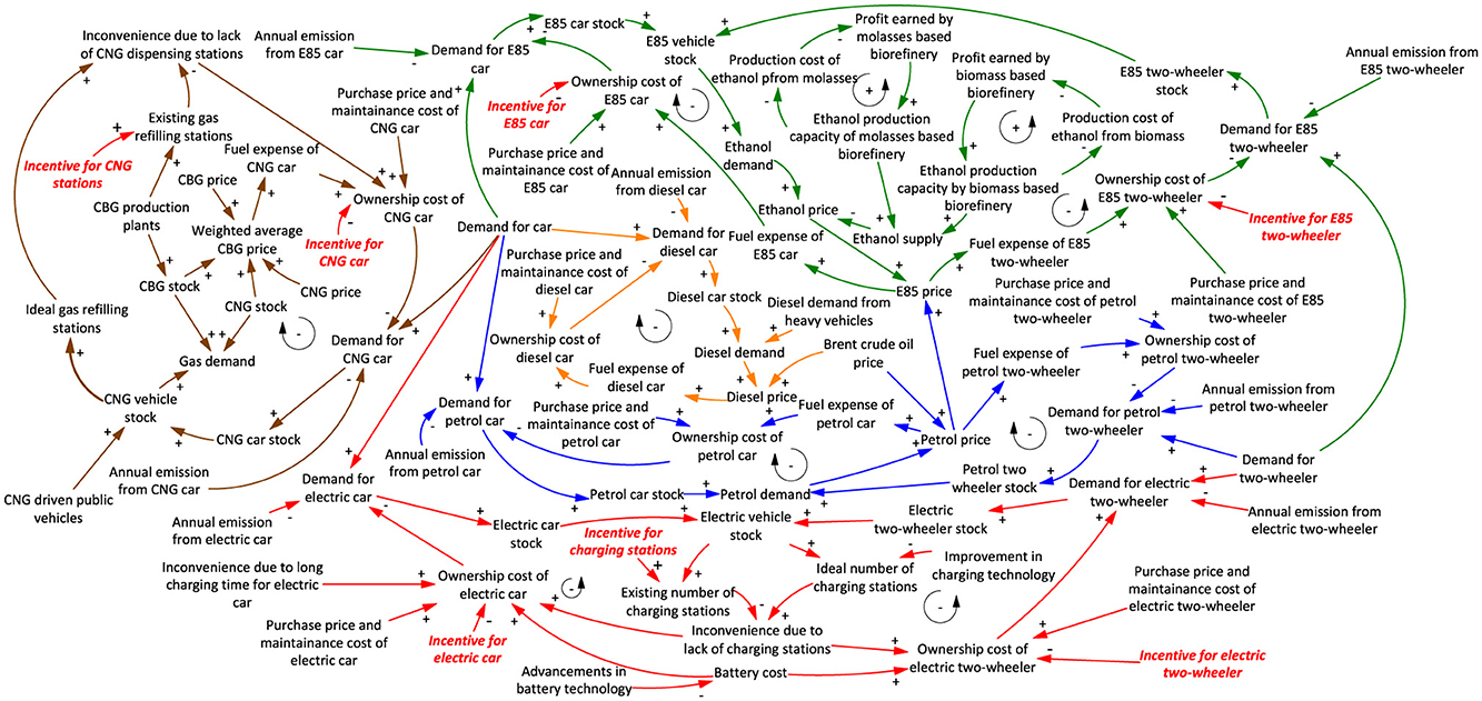
Figure 1. The causal loop diagram of the system dynamics model, as presented in the study by Saraf and Shastri (2024), has been modified to incorporate vehicle and infrastructure incentives. These incentive variables are highlighted in red color.

The ownership cost of a vehicle is the sum of the annualized vehicle purchase price, annual fuel expenses, and annual maintenance costs. Vehicle fuel expenses are influenced by fuel prices, which, in turn, are affected by fuel demand and supply. Higher fuel demand increases fuel prices, whereas higher fuel supply lowers the prices. The model captures these dynamics for petrol, diesel, and ethanol (E85). The production of ethanol, using molasses and lignocellulosic biomass as feedstock, is also considered in the model. As production capacity expands, experience in process technology improves, leading to a reduction in production costs. Reduced production costs increase profits, which, in turn, drive further increases in production capacity, creating positive feedback loops.

In the case of EVs and CNG vehicles, the lack of sufficient charging and gas-refilling stations poses a barrier to adoption. This inconvenience is measured by comparing the actual number of stations to the ideal number required for timely refueling or charging. The inconvenience cost is quantified and added to the ownership cost of these vehicles. Negative feedback loops are established between vehicle stock, ideal number of refueling stations, inconvenience cost, ownership cost, and vehicle demand. The new demand for each option alters the respective vehicle stock, which affects fuel demand for the next year. The simulations are done at an annual time step.

The annual GHG emissions of a vehicle option include the emissions during the operations stage and emissions during the production of fuel or energy sources such as petrol, diesel, ethanol, CNG, CBG, and electricity. For EVs, the GHG emissions during the manufacture and recycling/disposal of the lithium-ion battery are also considered. Four categories of consumers with different relative importance for cost and GHG emissions are modeled (Saraf and Shastri, 2024). Here, it is assumed that the distribution of consumers among these different categories does not change with time.

A detailed description of the model and the values for all the model parameters are provided in Saraf and Shastri (2023, 2024).

The next section discusses the optimization model formulation based on this SD model. It must be noted that this model does not have public transport as an option.

4 Formulation 1: optimization model without metro transportation

There are two different variations of this particular optimization model formulation. In both cases, the decision variables are annual investments across different vehicle technology options and infrastructure considered in the SD model. The first model minimizes the total investment over the simulation horizon to achieve a specific GHG reduction target at a particular time in the future. The second model, in contrast, minimizes the GHG emission in 2050 from the private transport sector. In this model, the total investment is not constrained. The second problem, therefore, provides an optimistic view of how much GHG emission reduction can be achieved, ignoring the financial constraints.

The vehicle incentives, delivered through annual tax discounts throughout the vehicle's service life, are aimed at lowering these novel vehicles' overall annual ownership costs. On the other hand, infrastructure investments focus on promoting the development of EV charging and CNG stations. These are one-time capital investments during the construction of these infrastructures. The infrastructure investment will reduce the inconvenience cost, increasing its annual demand (Figure 1).

Figure 2 is a schematic representation of the interaction between the optimization and the system dynamics model for the model of incentive minimization. The investment decisions are passed on to the SD model, which is simulated to determine the GHG emissions. The GHG emissions are compared with the target GHG emissions, and constraint satisfaction is checked. If the constraint is not met, the optimization algorithm modifies the decision variables (investments). Thus, the complete SD model functions as a set of constraints for the optimization model. The second model also has a similar strategy for GHG minimization.

Figure 2

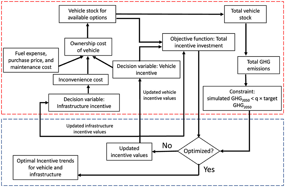
Figure 2. Schematic representation of the interaction between optimization and system dynamics model in minimizing the total incentive value while achieving the GHG emission reduction target. The Red dashed box represents the system dynamics model, while the blue dashed box represents the optimization model.

Both formulations also include constraints on the rate at which investment values can change. This is done to capture the practicality of changing investment prioritization in a government set-up. Generally, these decisions do not change drastically from year to year. If such constraints are not enforced, then the profile of investment decisions may be erratic and fluctuate rapidly. Although mathematically it might be an optimal solution, it will have little practical value. Therefore, enforcing this constraint results in a solution with greater acceptability and a greater likelihood of adoption. Investments for each type also have an upper bound. Additionally, as explained later, specific constraints are added for each of the two formulations. The optimization solver iteratively accesses and simulates the SD model and changes the decision variable values until the optimal solution is achieved.

The subsequent section gives the mathematical formulation for the two variations of the formulation.

4.1 Problem 1: minimization of total investment

The objective function to minimize the total investment over the simulation horizon is given by Equation 1.

$\begin{array}{ll}J=min{\displaystyle \sum _{t=1}^T}({\displaystyle \sum _{i=1}^m}({\displaystyle \underset{i}{\overset{t}{z}}}\times {\displaystyle \underset{i}{\overset{t}{V}}})+{\displaystyle \sum _{j=1}^n}{\displaystyle \underset{j}{\overset{t}{y}}})& (1)\end{array}$

where, the simulation time step is denoted by the subscript t, ranging from 1 to T, while the vehicle options are indicated by the superscript i, with the number of options ranging from 1 to m. Regarding refueling infrastructure, superscript j is used, with options ranging from 1 to n. $z_i^t$ is the incentive amount for i^th vehicle option at time step t, $V_i^t$ is the vehicle stock for i^th vehicle option at time step t, and $y_j^t$ is the incentive for setting up of infrastructure for j^th vehicle option at time step t.

The limits on the rate of increase and decrease of vehicle incentives are enforced through Equations 2, 3.

$\begin{array}{ll}{z}_i^t<p\times z_i^{t-1}\forall i,\forall t& (2)\end{array}$

$\begin{array}{ll}r\times z_i^{t-1}<z_i^t\forall i,\forall t& (3)\end{array}$

where, p represents the maximum increase in incentive over the previous time step, while r represents the maximum decrease in incentive over the previous time step. Similar constraints are also enforced on the infrastructure investment and are represented by Equations 4, 5.

$\begin{array}{ll}{y}_j^t<u\times y_j^{t-1}\forall j,\forall t& (4)\end{array}$

$\begin{array}{ll}v\times y_j^{t-1}<y_j^t\forall j,\forall t& (5)\end{array}$

where, u and v represent the maximum limit on the increase and decrease of infrastructure investments in consecutive years.

The estimation of GHG emission from the SD model is expressed in Equation 6, and the constraint representing a minimum reduction in GHG emission is expressed in Equation 7.

$\begin{array}{ll}GH{G}^t=g(z_i^t{y}_j^t,\alpha ,\beta )\forall t& (6)\end{array}$

$\begin{array}{ll}GH{G}^{\bar{t}}<q\times GH{G}_{ref}^{\bar{t}}& (7)\end{array}$

where, GHG emissions at time step t, denoted as GHG^t, are derived through a system dynamics simulation represented by $g(z_i^t,y_j^t,\alpha ,\beta )$. α and β are the variables and inputs of the SD model, respectively. It is crucial to emphasize that the variables (i.e., α) employed in the system dynamics model are simulated internally in the SD model and are not a part of the optimization model. $GH{G}_{ref}^T$ is the reference GHG emission at time step $\bar{t}$.

4.2 Problem 2: minimization of GHG emissions

This formulation is very similar to the previous one, with the only difference being the objective function. Instead of investment minimization, the objective function is GHG minimization in 2050. Since GHG is now an objective, there is no constraint on its value. The objective function is shown by Equation 8:

$\begin{array}{ll}J=min(GH{G}^t)& (8)\end{array}$

The remaining constraints, except the one involving GHG emissions, are same as those for problem 1.

The model developed and presented here is applied to the Indian context. Details regarding this application are discussed in the subsequent section.

4.3 Model parameterization for Indian transport sector

As mentioned earlier, the Indian government has been encouraging the adoption of novel vehicles by setting targets and providing incentives through various policies. Regarding electric vehicles, the FAME scheme offers an incentive of INR 15,000 per unit of battery capacity for electric vehicles at the time of purchase (Govt of India, 2015). Based on the average battery capacities of electric cars and two-wheelers, this incentive amount corresponds to 32% of the EV purchase price in 2022. Currently, no direct incentives are proposed for the purchase prices of E85 and CNG vehicles. The model, however, considers incentives for E85 and CNG vehicles also as decision variables. To maintain consistency among different variables, initial guess values for incentives for all non-petrol and non-diesel vehicle options are set at 32% of their purchase prices in 2022. Since the model simulations are done on an annual time-step and the annual cost of ownership is the factor governing vehicle purchase decision, the incentive is also annualized over the vehicle's service life. Purchase prices and service life data for novel vehicle options are taken from Saraf and Shastri (2023). Moreover, according to the FAME scheme, the maximum incentive can reach up to 40% of the purchase price of an electric vehicle (Govt of India, 2015). Based on this, the upper limit for vehicle incentives is 40% of the vehicle's purchase price. Note that the upper limit and vehicle purchase price are also adjusted for inflation. The inflation rate is assumed to be 3.5% (Saraf and Shastri, 2023). This upper limit is also annualized in accordance with the service life of the vehicle.

For promoting the development of charging infrastructure, the Indian government provides support in the form of property tax rebates, exemption from electricity costs during the construction phase, and a subsidy on the capital cost of the station (Moneycontrol, 2021). It is assumed that for every INR 500,000 subsidy, one charging station can be established (Moneycontrol, 2021). The charging station incentive for the first year is set at INR 150 Million which results in the establishment of 300 charging stations (Press Information Bureau, 2022). The upper limit on this incentive is considered to be INR 1 Billion, which corresponds to 2,000 new stations (The Economic Times, 2023a). This value is adjusted to account for inflation each year. In the case of CNG station incentives, a subsidy of INR 35 Million is provided to establish one station (IOCL, 2023). The CNG station incentive for the first year is set at INR 10.50 Billion, which corresponds to 300 stations. The upper limit for the establishment of CNG stations is also set to match that of charging stations, i.e., 2,000 stations. This translates to a maximum budget of INR 70 Billion. This upper limit is also adjusted annually to account for inflation.

p is assumed to be 1.2, implying that the incentive at time step t can increase up to 20% compared to the previous time step. The value of r is assumed to be 0.8, indicating a maximum reduction by up to 20% over the incentive value in the previous years. Similarly, the values of u and v are also assumed to be 1.2 and 0.8, respectively. This assumption is based on the observation that most policy shift happen gradually, and drastic changes are unlikely. For instance, FAME II funding increased by 11.5% in 2023, from INR 100 billion to INR 115 billion (Ministry of Heavy Industries, 2023). Additionally, funding for charging stations saw a 20% reduction, from INR 10 billion in 2022 to INR 8 billion in 2023 (Ministry of Heavy Industries, 2022, 2023). Moreover, the incentives for electric two-wheelers decreased by 33.33%, from INR 15,000 per kWh in 2022 to INR 10,000 per kWh in 2023 (Ministry of Heavy Industries, 2021, 2022, 2023). Based on these rates of change, the values for parameters p, r, u, and v are assumed.

A base scenario is first simulated without any incentives, and captures business as usual case. For problem 1, the GHG emissions reduction target for the year 2050 is defined in terms of the GHG emissions in the year 2050 for the base case ($\bar{t}=T$). In the base scenario, the GHG emissions in 2050 were 577.42 Mt CO₂e. Therefore, $GH{G}_{ref}^{\bar{t}}$ in Equation 7 is 577.92 Mt CO₂e. This model is applied to achieve a 5% reduction from this baseline level. Thus, q is taken as 0.95, resulting in target maximum GHG emissions of 549.02 Mt CO₂e. The solutions of the optimization problems are compared with the base case.

5 Formulation 2: optimization model with metro transportation

This section first describes the integration of metro transportation into the existing SD model, then presents the optimization model formulation for the revised model.

5.1 Inclusion of metro transport in system dynamics model

The SD model has been revised to simulate the impact of investments in metro lines. The fund invested in constructing metro lines is the input to the model. Figure 3 illustrates the SD model related to metro investment. As shown in Figure 3, the annual investment in the metro rail project is an input to the SD model. It is distributed between the funds for operating the existing metro lines and constructing new ones. Due to the complex nature of infrastructure development, including erection and commissioning phases spanning multiple years, it takes time for the investment to result in the construction and operation of the new lines. This time delay is indicated in Figure 3 by parallel lines on the arrow connecting investment to new metro line construction.

Figure 3

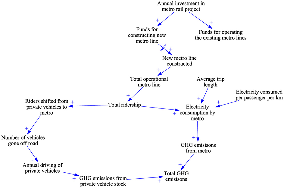
Figure 3. CLD showing variables and their corresponding causal relation involved in metro transportation.

It is assumed that increased accessibility to metro travel increases metro ridership. The new metro riders include those who have transitioned to metro transport from private vehicles, other public transport options, or walking. The scope of this study is limited to those riders who have switched from their private vehicles to metro transport. It is assumed here that consumers will still purchase private vehicles for specific uses such as recreation but will transition to the metro for daily use. Therefore, the demand for vehicles does not change.

An increase in the number of metro riders has two conflicting effects. It reduces the number of on-road vehicles. Thus, the total driving of a private vehicle is reduced. This reduces GHG emissions from private vehicle stock (Figure 3). However, the operation of a metro network requires energy. Therefore, increased construction and use of metro networks result in increased electricity consumption, thereby increasing GHG emissions in the sector. The actual energy consumption depends on the average trip length and the electricity consumption intensity of the metro lines. Both these effects are captured in this work (Figure 3). As the scope of this study is limited to the GHG emissions from private vehicles, the GHG emissions from metro operations corresponding to only those riders who have transitioned from their private vehicles to the metro are considered. Thus, it captures the change in GHG emissions resulting from the transition to metro transport from private vehicles. The total metro ridership also determines the total electricity consumption during metro operation. As the electricity consumption increases, the total electricity cost for operating the metro line increases, thereby increasing the metro operating fund.

5.2 Modeling of metro transport in SD model

The division of total annual investment in metro rail projects between the construction of new lines and operations of existing lines is shown in Equation 9.

$\begin{array}{ll}{I}_{tot}^t=I_c^t+I_o^t& (9)\end{array}$

where, $I_{tot}^t$, $I_c^t$, and $I_o^t$ are the annual investment for metro rail projects, funds allocated for constructing new metro lines, and funds allocated for operating the existing metro lines at time step t, respectively. The estimation of the length of the new metro line constructed corresponding to $I_c^t$ with time delay is calculated as per Equation 10.

$\begin{array}{ll}{L}_{new}^{t+a}=b\times I_c^t& (10)\end{array}$

where, $L_{new}^{t+a}$ is the new metro line constructed at time step t + a due to investment in time step t. Here, a is the time delay in constructing and commencing the operation of the new metro line. b represents the length of the metro line constructed per unit investment in metro construction. The new metro line constructed increases the total operational metro line as shown in Equation 11.

$\begin{array}{ll}{L}_{tot}^t=L_{tot}^{t-1}+L_{new}^t& (11)\end{array}$

where, $L_{tot}^t$ is the total operational metro length at time step t. The metro ridership as a function of operational metro length is determined as follows:

$\begin{array}{ll}{R}_{tot}^t=c\times L_{tot}^t& (12)\end{array}$

where $R_{tot}^t$ is the total metro ridership at time step t, and c is the parameter representing the number of metro riders per unit metro length. Equations 13, 14 show the estimation of riders transitioning from private cars and two-wheelers to metro transport, respectively.

$\begin{array}{ll}{R}_c^t=R_{tot}^t\times S_c& (13)\end{array}$

$\begin{array}{ll}{R}_{tw}^t=R_{tot}^t\times S_t& (14)\end{array}$

where, $R_c^t$ and $R_{tw}^t$ are the riders shifted from their private cars and two-wheelers to the metro transport at time step t, respectively, S_c and S_t represents the fraction of riders transitioned from private car and two-wheeler to metro transport, respectively. Equations 15, 16 estimate the number of cars and two-wheelers gone off the road, respectively.

$\begin{array}{ll}{C}^t=\frac{R_c^t}{O_c}& (15)\end{array}$

$\begin{array}{ll}{T}^t=\frac{R_{tw}^t}{O_{tw}}& (16)\end{array}$

where, C^t and T^t are the number of cars and two-wheelers gone off the road, respectively, at time step t. O_c and O_tw are the average occupancy of cars and two-wheelers, respectively. The annual driving of C^t and T^t is reduced due to the transition of riders to metro transport. The SD model is formulated based on the assumption that all private cars have equal annual driving distances, as do all two-wheelers. Here, C^t and T^t have lower annual driving than the other vehicles in stock. However, to simplify the formulation in the model, rather than specifying a low annual driving for individual vehicles C^t and T^t, an average reduction in annual driving for cars and two-wheelers is estimated. Equations 17, 18 show the average reduction in annual driving per car and two-wheeler, respectively.

$\begin{array}{ll}R{d}_c^t=\frac{C^t\times T_{avg}}{c{s}_{tot}^t}& (17)\end{array}$

$\begin{array}{ll}R{d}_{tw}^t=\frac{T^t\times T_{avg}}{tw{s}_{tot}^t}& (18)\end{array}$

where, $R{d}_c^t$ and $R{d}_{tw}^t$ is the average reduction in annual driving of cars and two-wheelers at time step t, respectively. T_avg is the average metro trip length and $c{s}_{tot}^t$ and $tw{s}_{tot}^t$ are the car and two-wheeler stock at time step t. The numerator in RHS represents the total driving distance reduced due to the transition of riders from private vehicles to metro transport. The average reduction in annual driving of cars and two-wheelers is deducted from the annual driving of respective vehicles estimated in Saraf and Shastri (2023) to estimate the annual driving of vehicles as riders transition from private vehicles to metro transport. Equations 19, 20 show the estimation of the annual driving of cars and two-wheelers, respectively.

$\begin{array}{ll}{D}_{c_{new}}^t=D_c^t-R{d}_c^t& (19)\end{array}$

$\begin{array}{ll}{D}_{t{w}_{new}}^t=D_{tw}^t-R{d}_{tw}^t& (20)\end{array}$

where, $D_{c_{new}}^t$ and $D_{t{w}_{new}}^t$ are the annual driving of cars and two-wheelers at time step t, respectively. $D_c^t$ and $D_{tw}^t$ are the annual driving of cars and two-wheelers at time step t, respectively, as estimated in Saraf and Shastri (2023).

Equation 21 shows the estimation of electricity consumption during metro operation. Consequently, the electricity cost and operating cost of the metro also increase as shown in Equations 22, 23, respectively.

$\begin{array}{ll}{E}_c^t=R_{tot}^t\times T_{avg}\times e& (21)\end{array}$

$\begin{array}{ll}{E}_p^t=E_c^t\times p& (22)\end{array}$

$\begin{array}{ll}{I}_o^t=E_p^t\times f& (23)\end{array}$

where $E_c^t$ is the electricity consumed during metro operation and e represents the electricity consumed per rider per unit trip length. $E_p^t$ is the total electricity cost corresponding to $E_c^t$, and p is per unit electricity price. As the electricity cost increases, the operating cost increases by a factor of f.

5.3 Metro model parameterization

In India, the metro systems in Delhi and Mumbai are the most extensive. Consequently, data on these metro lines related to investment in metro construction, the length of new metro lines, annual ridership, average trip length, and annual electricity consumption were gathered (Maharashtra Government, 2023; DMRCL, 2023; The Times of India, 2021) and fitted to estimate the values of model parameters.

Supplementary Table S1 the construction period, investment, and length of various metro lines. Based on this, it is assumed that it takes five years for the metro to be operational from the time of the first investment (a = 5). The investment values (inflated to the present value of money) and the length of the metro line constructed corresponding to various metro lines (in Supplementary Table S1) are used to estimate the average length of the metro line constructed per unit investment. The value of parameter b is 0.0034 km/INR 10 Million investment. In 2019–20, Bengaluru's daily ridership per kilometer was 9,456. Likewise, in Delhi, Mumbai, and Chennai, it reached 40,650, 14,653, and 2,553, respectively (The Times of India, 2021). The parameter c is determined by calculating the average of these values, which is 16,828. Sharma et al. (2014) reported that in Delhi, about 30% and 40% of commuters have shifted from their private vehicles to the metro in 2006 and 2011, respectively. Similarly, Soni and Chandel (2018) conducted a survey in Mumbai in 2018 in all the 12 metro stations to identify the fraction of commuters using private vehicles before the Mumbai metro. They found that about 8% of commuters shifted from cars and two-wheelers to metro transport. Based on the survey data, the values for S_c and S_t are assumed to be 0.15. The average occupancy of cars and two-wheelers, i.e., O_c and O_tw are taken as 2.4 and 1.5 passengers per vehicle, respectively (Soni and Chandel, 2018). Soni and Chandel (2018) reported the average metro trip length in Mumbai as 6 km, while Sharma et al. (2014) reported the average metro trip length in Delhi in 2006 and 2011 as 10 km and 12.5 km, respectively. Based on these values, this study's average trip length (T_avg) is assumed to be 16 km. Based on the ridership and annual electricity consumption data collected for the Mumbai Metro (Soni and Chandel, 2018), the value of e is estimated to be 0.034 kWh/passenger-km. The electricity price p is estimated in the SD model. As per the data reported for the Delhi metro, the electricity cost constituted 30% of the total operational cost of the metro (Goel and Tiwari, 2014). Therefore, the value of f is taken as 3.3.

Several parameters of the modified SD model related to the metro system are not known with a high degree of certainty. Acquiring data from other cities or obtaining additional data from the metro lines in Delhi and Mumbai proved challenging. The values of these parameters may also change with time as metro systems become common in more cities in India. Consequently, sensitivity analysis has been carried out on these model parameters to assess how changes in parameter values may impact the change in GHG emissions in 2050. The details of the sensitivity analysis will be elaborated upon in the subsequent sections.

5.4 Optimization problem formulation

The optimization model formulation is the same as in the previous section. The goal is to derive optimal investment strategies to minimize GHG emissions by 2050. The formulation described in the minimization of GHG emissions in Section 4.2 is applied. The system dynamics model, acting as a constraint in the optimization model, has been modified to integrate metro transportation. Initial guesses, upper and lower bounds, and other financial constraints are the same as described in the Section 4.3.

The initial aim was to include metro investment also as a decision variable in addition to the ones considered previously. The optimization model was accordingly modified. However, the resulting optimization problem encountered numerical issues. The metro investment was numerically very high as compared to the other investments. Additionally, the problem is non-convex in nature due to the presence of nonlinear equality constraints. Therefore, the optimization problem was encountering convergence issues. Several strategies, such as scaling of decision variables, modifying the convergence and optimality tolerances, and adjusting the step size of the solver, were attempted. The numerical issue, however, could not be addressed. Consequently, the approach was modified. Instead of considering metro investment as a decision variable, three different metro investment patterns were considered, and the optimization problem was solved to determine values (trends) for the remaining decision variables, namely, vehicle incentives and infrastructure investment.

The different scenarios considered here, including the three different metro investment possibilities (Supplementary Figure S1), are explained here:

• No metro investment scenario: This scenario replicates the minimum GHG emission scenario outlined in Section 4.2. It forms the foundation for understanding the impact of investing in metro transportation on incentives for novel vehicle options, their adoption trends, and GHG emissions.

• Low metro investment scenario: In this scenario, a linear trajectory is assumed for the investment in metro transportation that starts from INR 200 Billion, per the Indian budget (The Economic Times, 2023c), and reaches INR 8.6 Trillion in 2050.

• High metro investment scenario: In this scenario, a linear trajectory is assumed for the investment in metro transportation that starts from INR 200 Billion and reaches INR 50.6 Trillion in 2050.

• Decarbonization scenario: This scenario is similar to the high metro investment scenario, including early awareness of consumers and greater penetration of renewables in the electricity grid as discussed in Saraf and Shastri (2024).

Since the SD model was developed in MATLAB ^®. The optimization model was also formulated in MATLAB ^®. The simulation and optimization horizon was from 2023 to 2050, and the simulation time step was one year. Sequential quadratic programming (SQP) algorithm in fmincon solver was used to solve the optimization problems. The maximum number of iterations was set at 100,000. The step, optimality, and constraint tolerance values were set at 1e-18. Generally, it took around 2,000 iterations to solve the problem.

6 Results and discussion

The results for formulation 1 are first discussed followed by results for formulation 2 with metro transport option.

6.1 Formulation 1: optimization problem without metro transportation

This section presents the results of the optimization problems discussed in Section 4. Since the results of the optimization model are compared with the base case, the simulation results for the base case are first presented.

6.1.1 Base case

For the base case, the adoption of novel vehicle options among cars and two-wheelers was 37.62% by 2050. Figure 4 shows the share of various options in total car stock in 2050. Petrol was the most preferred option, followed by E85, diesel, CNG, and electric vehicles. Consequently, the GHG emissions in 2030 reached 391.7 Mt CO₂e and plateaued at 577.92 Mt CO₂e in 2050. Saraf and Shastri (2024) estimated that the GHG emissions for the private road transport sector in 2030 should be 263 Mt CO₂e to meet the COP26 emission reduction target. However, the base scenario surpasses this target by 128.7 Mt CO₂e.

Figure 4

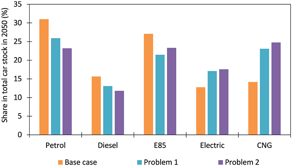
Figure 4. Share of various car options in total car stock in 2050.

6.1.2 Problem 1: minimization of total investment

The optimal solution recommended a total investment of INR 15 Trillion over the entire simulation horizon. Almost 92% of this total investment (INR 13.8 Trillion) was for vehicle incentives, while the rest was for infrastructure. Figures 5, 6 show the incentive trends for cars and two-wheelers, respectively. It was observed that the incentive for electric cars and two-wheelers increased at the maximum possible rate given the constraints till 2027 and 2028, respectively. Thereafter, the incentives were reduced rapidly, again limited by the limit on the rate of reduction. The incentive values for other car and two-wheeler options were reduced from the beginning of the simulation. Figure 7 shows the incentive trends for EV charging and CNG refueling infrastructure. Note that the y-axis of this figure has a logarithmic scale. As can be seen, the incentive trends for both increased at the maximum possible rate till 2036 and then rapidly reduced thereafter.

Figure 5

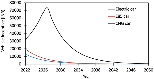
Figure 5. Incentive trends for E85, EV, and CNG four-wheelers to minimize total investment.

Figure 6

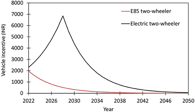
Figure 6. Incentive trends for E85 and electric two-wheelers to minimize total investment.

Figure 7

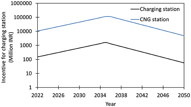
Figure 7. Incentive trends for charging and CNG refilling stations to minimize total investment. Note that the y-axis of this figure has a logarithmic scale.

As per these trends, electric vehicles should be aggressively promoted for the next few years by giving incentives for vehicle purchases and rapidly developing the charging infrastructure to support them. This is reflected in the rapid increase in the adoption of EVs in the near future. Supplementary Figure S2 shows the share of new car sales in the annual total car sales for different years. The fraction of electric car sales in total annual sales of new cars increased from 11.4% in 2022 to 48.35% in 2028, significantly higher than a mere 14% in 2028 for the base case. The share of various car options in total car stock in the year 2050 is shown in Figure 4. It shows a reduction in the share of petrol, diesel, and E85 cars as compared to the base case, while that of EVs and CNG cars increased. Due to vehicle incentives and infrastructure investment, the share of novel vehicle sales increased from 24% in 2022 to 80% in 2030.

Supplementary Figure S3 compares the annual ownership costs of petrol and electric cars in this scenario with those in the base case. Without the incentive, petrol cars would have been preferred over electric cars due to lower annual ownership costs. Due to the reduced adoption of petrol vehicles (as shown in Figure 4), the petrol demand reduced, thereby reducing the petrol prices and annual ownership cost of petrol cars. Therefore, a slight reduction was observed in the annual ownership cost of petrol cars in this scenario compared to the base case. The aggressive incentivization of electric cars drastically reduced ownership costs, making petrol cars relatively less desirable. The proportion of petrol car sales in annual new sales reduced from 56.7% in 2022 to 11.4% by 2028.

CNG cars are not prioritized despite lower GHG emissions than petrol cars. This is because the vehicle selection is based on the vehicle's annual ownership cost and annual GHG emissions (Supplementary Figures S5–S7). It has been previously demonstrated that the cost of ownership of CNG cars is quite sensitive to the availability of CNG refueling infrastructure (Supplementary Figure S6). Due to the shortage of refueling stations, inconvenience costs increase, reducing demand. When the demand remained low for subsequent time steps, the CNG car stock also decreased, reducing the demand for gas-refilling stations and thus reducing inconvenience. This led to increased adoption of CNG car stock, and the feedback loop continued.

In such a situation, offering vehicle incentives to CNG cars could exacerbate the instability. Therefore, the optimization model prioritizes electric vehicles from 2022 to 2036 by providing vehicle and infrastructure incentives to reduce annual ownership costs and prevent the adoption of petrol cars. Meanwhile, it also prioritizes investment in gas refilling stations to develop a strong infrastructure network to support the high adoption of CNG cars. As seen in Figure 7, the investment in charging and CNG stations increased until 2036 and then reduced. This can be explained by Supplementary Figures S4, S8. The annual ownership cost of CNG cars became the lowest from 2035. As a result, the adoption of CNG cars increased from 9% in 2022 to 39% in 2042. Based on the specific GHG reduction target, there is no requirement to provide additional incentives for any options. Hence, incentive values started to decrease with the maximum limit.

In the base case, in 2023 and 2033, E85 car adoption accounted for 39% and 35% of the total car stock, respectively. However, despite experiencing a minor decrease to 35% in 2023 and 33.4% in 2033, the adoption of E85 cars remained substantial in this problem as well. After 2040, E85 cars emerged as the second most prevalent vehicle choice, following CNG cars. Although E85 cars exhibit reduced annual ownership costs and emissions, the optimizer did not prioritize incentives for E85 vehicles due to the potential for increased demand for ethanol with high adoption rates. The limited ethanol supply could result in unmet demand, leading to higher ethanol prices and annual ownership costs for E85 cars. Increase in the annual ownership cost will reduce the demand for E85 cars. Reduced demand, despite incentives for E85 vehicles, would hinder their adoption. Since E85 cars have lower greenhouse gas emissions, a decline in their adoption could make it difficult to meet the GHG emission reduction targets.

This situation is undesirable because E85 vehicles have lower greenhouse gas emissions.

6.1.3 Problem 2: minimization of GHG emissions

The minimum GHG emission in 2050 was achieved at 535.3 Mt CO₂e, with a total incentive investment of INR 137.74 Trillion over the entire simulation horizon. Approximately 98% of this amount was allocated to vehicle incentives, with the remaining portion designated for infrastructure incentives. The total investment has risen substantially from INR 15 Trillion to INR 137.74 Trillion, despite a minor reduction in GHG emissions from 549.02 Mt CO₂e to 535.5 Mt CO₂e in 2050. This non-linear trend can be attributed to the necessity of significantly increasing investment in the phase of high vehicle demand to ensure greater adoption of novel vehicles, thereby reducing GHG emissions.

The trends in vehicle and infrastructure incentives are depicted in Figures 8, 9, respectively. The justification for the trends is similar to that for problem 1 since the vehicle cost and emission attributes are the same. The incentives for electric cars increased until 2034 and then decreased. Similarly, incentives for charging stations also increased until 2030 and then decreased. The incentive for E85 vehicles increased till 2026, ensuring a higher adoption of E85 cars until the annual ownership cost of CNG cars stabilized. The fraction of E85 cars in total car sales in 2026 was 53.3% (Supplementary Figure S9). For CNG cars, as explained in the preceding section, offering vehicle incentives can destabilize the annual ownership cost, leading to a decline in the adoption of CNG cars. Hence, the vehicle incentive was initially reduced while providing incentives for setting up gas refilling stations at the maximum limit. Once a sufficient infrastructure network was established, the vehicle incentive aimed to decrease the annual ownership cost of CNG cars to the minimum, thereby increasing their adoption. Supplementary Figure S10 shows that after 2034, CNG cars had the lowest annual ownership cost. The fraction of CNG car sales in total car sales in 2037 was 49%.

Figure 8

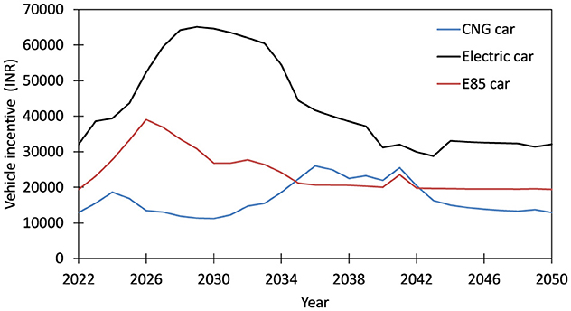
Figure 8. Incentive trends for E85, EV, and CNG four-wheelers to minimize GHG emissions.

Figure 9

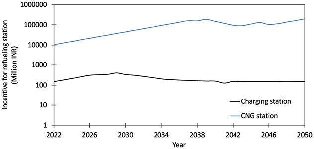
Figure 9. Incentive trends for charging and CNG refilling stations to minimize GHG emissions. Note that the y-axis of this figure is a logarithmic scale.

If constraints on the rate of increase or decrease were removed, the GHG emissions could reduced to 522.5 Mt CO₂e in 2050 with a total investment of INR 129 Trillion, with 86.7% allocated to vehicle incentives and the remaining portion dedicated to infrastructure investments. This result is expected since the optimization model is less constrained. As expected, the incentives had very aggressive profiles. For example, the investment trends hit very high values in the initial phase of the simulation, reducing the inconvenience costs to zero for EVs and CNG vehicles (Supplementary Figures S11, S12). The CNG car sales in total annual new car sales increased to 57.3% and that for petrol reduced to 6% in 2030.

Based on the results of Problem 1 and Problem 2, it can be inferred that a trade-off exist between the investment in incentives and the reduction in GHG emissions which is achieving higher emission reduction is more expensive. To understand the trade-off clearly, Problem 1 was reformulated and solved for varying values of q, i.e., 1%, 3%, 6%, and 6.8% and the resultant values of investment in incentives were plotted against the GHG emissions in 2050. Figure 10 shows the Pareto curve between the investment and GHG emissions in 2050. The results also showed diminishing returns. The reduction of GHG emissions from 577.92 Mt CO₂e to 549.02 Mt CO₂e, i.e., 28.9 Mt CO₂e, was achieved with an investment of INR 15 trillion, meaning that every INR 1 trillion investment reduced the GHG emissions by 1.92 Mt CO₂e. However, the reduction of GHG emission below 549.02 required much higher investment. Every INR 1 trillion investment could only reduce 0.11 Mt CO₂e. The constraints on incentive changes and the upper limit on incentives led to increased investment requirements for achieving greater GHG emission reductions. Furthermore, the initial phase of the simulation saw low adoption of novel vehicles due to high purchase prices and limited refueling infrastructure, resulting in continued adoption of petrol and diesel vehicles, which then remain in use for their full service life. Thus, promoting the adoption of novel vehicles early on is crucial.

Figure 10

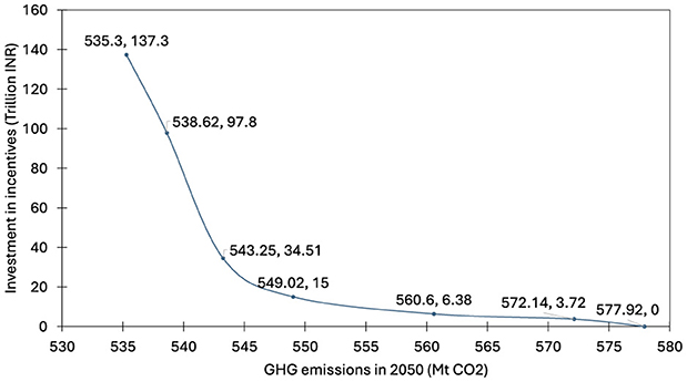
Figure 10. Pareto curve between the investment in incentives and the GHG emissions in 2050.

6.2 Formulation 2: optimization problem with metro transportation

This section presents the results of the optimization problems discussed in Section 5.

6.2.1 Simulation and sensitivity analysis

Simulation studies were performed before using the revised model with the metro transport option in the optimization formulation. The purpose of the simulation studies was to establish a base case or benchmark for the revised model. Additionally, sensitivity analysis was performed to determine the impact of some assumptions made during model parameterization.

The baseline scenario was devised assuming a linear trajectory for the investment in the metro, starting at INR 20,000 Billion in 2022 as per the Indian budget 2022–23 (The Economic Times, 2023c). The base case assumes that it will reach 8.6 trillion INR in 2050. No incentives for individual vehicles were considered, and the consumer environmental awareness factors were the same as those for the base case in the previous scenarios. Simulation results showed that the annual GHG emissions in 2050 were 562.7 Mt CO₂e. These were lower than 577.92 Mt CO₂e obtained for the base case scenario in the previous formulation when metro transport was not considered. This implied that even without incentives, transitioning towards metro transport can lead to a noticeable reduction in GHG emissions.

To explore the sensitivity of the GHG emissions to model parameters a, b, c as well as model inputs S_car and S_tw, the base values of these parameters (as discussed in Section 5.3) were varied from –50% to +50%. Each parameter was individually altered, and the resulting change in GHG emissions in 2050 was examined. Supplementary Figure S13 shows the sensitivity of GHG emissions in 2050 to model parameters. It can be observed from the figure that as the metro construction period increased by 50%, i.e., to 7.5 years, the resultant GHG emissions also increased by 0.53%. Similarly, as the length of the metro line constructed per unit investment was increased by 50%, the GHG emissions in 2050 were reduced by 1.5%. An increase in daily ridership per km reduced GHG emissions by 1.5%. Among the model parameters, the GHG emissions were most sensitive to the electricity consumption per passenger km. An increase in electricity consumption per passenger km by 50%, increased the GHG emissions by 1.6%, while a reduction in electricity consumption by 50%, reduced the GHG emissions by 1.8%, which was more significant than other model parameters. Using a renewable electricity grid for metro operations could significantly reduce GHG emissions.

6.2.2 Optimization results: GHG emissions and investment trends

Table 1 reports the minimum GHG emissions achieved in 2050 under various metro investment scenarios. Table 2 shows the distribution of the total investment in novel transport options across different categories for various metro investment scenarios. A substantial decrease in GHG emissions occurred from the no metro investment to the low metro investment scenario, dropping from 535.5 to 464.5 Mt CO₂e. This was because metro transportation can significantly reduce the driving of private vehicles while emitting lower emissions per unit distance traveled. In the low metro investment scenario, the driving distances for private cars and two-wheelers reduced by 645 km per vehicle and 601 km per vehicle by 2050, respectively. This resulted in an increase in GHG emissions of 11.3 Mt CO₂e due to metro operations in 2050. This was compensated by the significant reduction in GHG emissions from on-road vehicles, thereby giving a 20% reduction over the scenario with no metro investment and no incentives. The reduction was about 13% compared to the scenario with no metro investment but investment in other incentives. The GHG reduction intensity was 0.3 Mt CO₂e per INR Trillion investment for the no metro investment scenario. This increased to 0.44 Mt CO₂e per INR Trillion investment for low metro investment scenarios. It clearly shows that investment in public transport infrastructure and incentives for novel vehicles leads to more impact. About 96% of the total investment of INR 128.25 Trillion was allocated to vehicle incentives and the rest to infrastructure investments. The vehicle incentives were distributed between electric, CNG, and E85 vehicles with a share of 51%, 42%, and 7%, respectively. Among the infrastructure investments, investments for gas refilling stations dominated over charging stations. Since there was a significant benefit in the low metro investment scenario, it was expected that the benefit would be even greater when there was substantially higher investment in the metro. Instead, GHG emissions in 2050 increased slightly to 467.8 Mt CO₂e in the high metro investment scenario compared to the low metro investment scenario. This seemed counterintuitive, but it can be justified as follows.

Table 1

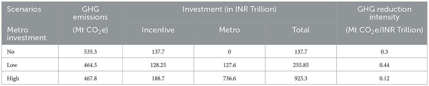
Table 1. GHG emission and incentive investment in different scenarios for formulation 2 with metro transport option.

Table 2

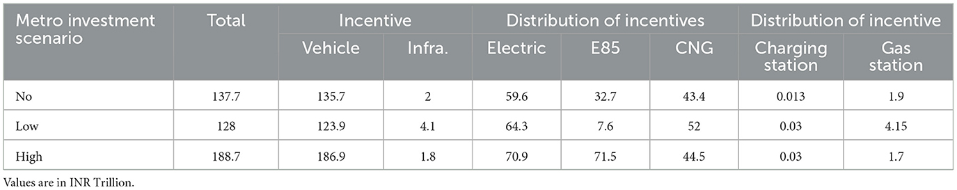
Table 2. Total incentive and allocation in vehicle and infrastructure incentive for different metro investment scenarios.

The investment for metro transportation activated a feedback effect in the system, as illustrated in Figure 11. With the reduction in private vehicle driving, fuel consumption was significantly reduced, particularly petrol consumption. In the transport sector, petrol is predominantly utilized by private vehicles, while diesel experiences its highest demand from heavy-duty vehicles. Consequently, any fluctuations in the demand for petrol vehicles or variations in annual driving habits carry substantial implications for both petrol demand and pricing dynamics. As outlined in Saraf and Shastri (2023), the decline in petrol demand led to a reduction in petrol prices, subsequently lowering the fuel expenses and annual ownership costs associated with petrol vehicles. Supplementary Figure S14 compares the annual ownership costs of a petrol car in different investment scenarios. Until 2030, there was no notable change in the annual ownership cost of petrol cars. However, after 2030, the difference began to increase significantly. The diminished annual ownership costs became an attractive factor for adopting petrol vehicles. Consequently, the adoption of novel vehicles decreased. However, increased adoption of petrol vehicles is not conducive to minimizing GHG emissions, given the higher GHG emission intensity of petrol compared to ethanol, CBG, and EVs. Therefore, there was a 47% increase in the incentives for different vehicle options (from INR 128.25 Trillion to INR 188.7 Trillion), yet the total emissions increased in the year 2050. The GHG emission reduction intensity was 0.12 Mt CO₂e per INR Trillion investment. To further verify this hypothesis, the SD model was simulated without incentives for novel vehicle options, using high investment in metro transportation as an input. The adoption of novel vehicle options declined from 43% to 37%, and the adoption of petrol vehicles increased from 53% to 57.2%. As a result, GHG emissions increased from 467 Mt CO₂e to 493 Mt CO₂e in 2050.

Figure 11

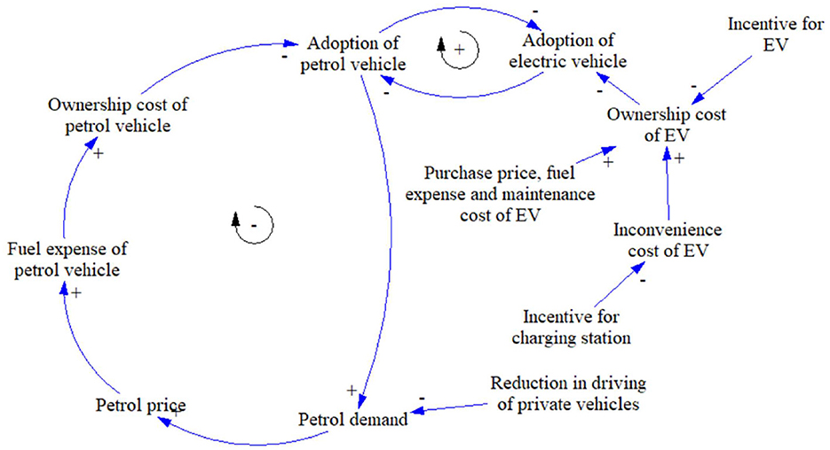
Figure 11. Causal loop diagram showing the impact of reduced driving on adoption of petrol vehicles.

This result captures the central hypothesis of this work, which is that the behavior of the transport sector can be highly non-linear. Results cannot be extrapolated, and consumer decision-making will be crucial in achieving the desired goals. The policy instruments, therefore, need to be designed appropriately. An optimization problem was solved to minimize the GHG emissions for a high metro investment scenario by including a carbon tax rate on transport fuels as discussed in Saraf and Shastri (2024). The results showed a decline in GHG emissions in 2050 from 467.8 Mt CO₂e in a high metro investment scenario to 456.33 Mt CO₂e. Additionally, the total investment reduced significantly from INR 188.7 Trillion in the high metro investment scenario to INR 66.86 Trillion. Out of this, about 98% was for vehicle incentives and the rest for infrastructure investment. Among the vehicle incentives, about 40% was allocated to CNG cars, followed by 30% to E85 vehicles and the rest to electric vehicles. Regarding the adoption of novel vehicle options, it increased from 43% in high metro investment to 46% in 2050 due to the imposition of the carbon tax (Supplementary Figure S15). The reduction in total investment when the carbon tax was imposed compared to the high metro investment scenario was to prevent the annual ownership costs of E85 and electric cars from becoming comparable with CNG cars, thereby ensuring high adoption of CNG cars. Supplementary Figure S16 shows the annual ownership costs of various car options. The investment in gas refilling stations was sufficient to ensure no inconvenience costs for CNG cars. Therefore, the annual ownership cost of the CNG car shows no fluctuations (see Supplementary Figure S16). In addition, lower carbon tax due to lower emissions and annual ownership cost made it the most preferred option. Due to the imposition of the carbon tax, the adoption of petrol cars declined. The fraction of petrol car sales in total car sales in 2030 reduced from 12% in the high metro investment scenario to 8.3%. As a result, higher investments were not required to prevent the adoption of petrol vehicles. In this particular case, the result shows that high metro investment will need to be complemented with carbon tax to keep fossil fuel-based vehicles more expensive to own. This is expected to provide significant benefits and will lead to a reduction in total GHG emissions.

6.2.3 Decarbonization scenario

An optimization problem was solved for the high metro investment scenario by including early awareness of consumers and greater penetration of renewables in the electricity grid as discussed in Saraf and Shastri (2024). Figure 12 shows the GHG emission trend for the decarbonization scenario. In 2030, GHG emissions reached 352 Mt CO₂e, still 34% higher than the COP26 target for the private road transport sector. However, the GHG emissions show a promising trend, peaking at around 2040 and then reducing for the remaining time horizon. Since the adoption of novel vehicles only began in 2022–23, conventional petrol and diesel vehicles still made up a significant share of the total vehicle stock, posing a challenge to meet the COP26 emissions reduction target by 2030. In 2023, the demand for novel vehicles was low at 5.48%, while conventional vehicles remained highly popular, with annual demands for petrol cars, two-wheelers, and diesel cars at 54%, 72.94%, and 18.3%, respectively. These conventional vehicles continued to operate until the end of their service lives. While incentives, carbon tax, greener electricity grid, and consumer awareness contribute to increased demand of novel vehicles, bringing their adoption up to 34% in total vehicle stock by 2030, the stock of petrol and diesel cars still held a substantial share of 32% and 15.5%, respectively in total car stock, accounting for nearly 50% of the total car stock. Thus, with novel vehicle adoption only starting in 2022–23, achieving the 2030 COP26 target is challenging. Banning the purchase of new petrol and diesel vehicles, or introducing an attractive vehicle scrapping/swapping policy could help bridge this gap.

Figure 12

Figure 12. GHG emission trend in decarbonization scenario.

In terms of investment, the incentive investment was INR 77.9 Trillion, significantly lower than that obtained in the high metro investment scenario, i.e., INR 188.7 Trillion. Reduction in investment was attributed to increased adoption of novel vehicle options due to increased environmental awareness and a greener electricity grid, leading to reduced emission intensity for electric vehicles. The vehicle incentive constituted 97% of the total investment and the rest for infrastructure investments. The highest share of vehicle incentives was 45.6% for E85 vehicles, followed by 31% for EVs and 23.4% for CNG vehicles. The adoption of novel vehicle options increased from 43% in the high metro investment scenario to 48% in the decarbonization scenario in 2050. In the decarbonization scenario, the share of E85 cars in the total car stock in 2050 was 32%, the highest among other available options, followed by CNG cars with 29.2% share and electric cars with 9.2%. The fraction of E85 car sales in total car sales has been highest at 48% among other vehicle options in 2030 (Supplementary Figure S17). As E85 cars had the highest preference during the phase of high vehicle demand, it led to a significant share in the total car stock. The fraction of CNG car sales in total car sales increased 16.6% in 2022 to 75.8% in 2050, which has been the highest among other vehicle options. Higher adoption of E85 and CNG vehicles due to lower annual ownership costs and emissions dominated the adoption of electric vehicles. In addition to that, EVs were less preferred due to their higher annual ownership costs and emissions compared to E85 and CNG vehicles. As a result, the share of electric cars in total car stock in 2050 was reduced to 9% from 18.3% in the high metro investment scenario. Even with comparable petrol prices, the fraction of petrol cars in total car sales throughout the simulation horizon was lower than in the high metro investment scenario.

A pivotal factor contributing to reducing GHG emissions was the decrease in GHG emissions from metro operations due to a greener electricity grid. The GHG emissions from metro operation in 2050 reduced from 104 Mt CO₂e in the high metro investment scenario to 0.08 Mt CO₂e in the decarbonization scenario. This indicates the importance of increasing renewable share in the electricity grid.

7 Conclusion

An optimal investment strategy has been devised to allocate the incentives for novel vehicle options to decarbonize the Indian private vehicle sector. This work has used a system dynamics model, previously developed for the private road transport sector of India, within an optimization modeling framework. Different optimization models with varying objectives and constraints were solved, and multiple scenarios were considered.

The critical overall conclusion from the results was that the sector is highly complex, with strong interactions between different vehicle technologies. Therefore, incentives must be designed to consider these interactions and the effects of feedback in the system. Otherwise, they are likely to be less effective. Incentivization strategy should be combined with carbon taxation and increased renewables in the electricity grid for maximum benefits.

Specifically, it was observed that a total investment INR 15 Trillion was needed to achieve the GHG emissions target of 549.02 Mt CO₂e by 2050. However, the investment rose by over 9 folds to INR 137.74 Trillion to achieve GHG emissions of 535 Mt CO₂e by 2050. This indicated a highly nonlinear nature of the GHG reduction and cost trade-off. EVs were incentivized in the near future to reduce the adoption of petrol and diesel vehicles, while incentives were provided to establish strong network of charging and gas-refilling stations. In the later stage, CNG vehicle were prioritized by removing the purchase incentives for other vehicle options. The rate at which incentives were increased or decreased impacted both the minimum achievable GHG emissions and the total investment required. A higher rate of increase of incentive especially during the phase of high vehicle demand can lead to greater GHG reductions due to the accelerated adoption of novel vehicles. Metro transport could significantly reduce GHG emissions due to the reduced use of vehicles. The GHG reduction benefit per unit of investment increased from 0.3 to 0.44 Mt CO₂e/INR Trillion when metro investment was an option. However, beyond a certain threshold of investment in metro transportation, it was needed to be supported by more significant incentives for novel vehicle options due to a feedback effect causing reduction in petrol price. Implementation of a carbon tax on transport fuels demonstrated effectiveness in reaching minimum GHG emission of 456.8 Mt CO₂e in 2050, along with a notable decrease in financial incentives by INR 66.8 Trillion. In addition to that, increased renewable share in the electricity grid and environmental awareness among consumers reduced the GHG emissions further to 400 Mt CO₂e in 2050. However, it was still higher than the COP26 emission reduction target of 2030 by 34%. Greener electricity grid reduced the emissions from metro transportation by 99% in 2050.

This work involved integrating metro transportation into the system dynamics model, introducing several new parameters, such as investment in metro line construction, length of operational lines, construction duration, daily ridership, and more. In order to model the dynamics of metro construction and its impact on daily ridership, most of the data needed for estimating parameter values were obtained from two major metro cities in India, Delhi and Mumbai. However, as metro lines continue to be constructed and become operational in additional cities, these parameter values would not be able to capture the dynamics of metro transportation at national level accurately. Thus, periodic re-parameterization will be necessary as more data becomes available.

The work can be extended further to consider other emerging technologies such as fuel cell vehicles. Other transport sectors, such as long-distance road transport (passenger and freight), can also be considered. Finally, this work considered only GHG emissions as the environmental impact. However, other pollution effects are equally important and can be considered in the vehicle purchase decision-making model.

Data availability statement

The original contributions presented in the study are included in the article/Supplementary material, further inquiries can be directed to the corresponding author.

Author contributions

NS: Conceptualization, Methodology, Writing – original draft. YS: Conceptualization, Methodology, Supervision, Writing – review & editing.

Funding

The author(s) declare financial support was received for the research, authorship, and/or publication of this article. This study was supported by the SPLICE - Climate Change Programme, Department of Science and Technology, Ministry of Science and Technology through project DST/CCP/CoE/140/2018 (G).

Conflict of interest

The authors declare that the research was conducted in the absence of any commercial or financial relationships that could be construed as a potential conflict of interest.

Publisher's note

All claims expressed in this article are solely those of the authors and do not necessarily represent those of their affiliated organizations, or those of the publisher, the editors and the reviewers. Any product that may be evaluated in this article, or claim that may be made by its manufacturer, is not guaranteed or endorsed by the publisher.

Supplementary material

The Supplementary Material for this article can be found online at: https://www.frontiersin.org/articles/10.3389/frsus.2024.1472115/full#supplementary-material

References

Ashok, B., Kannan, C., Usman, K. M., Vignesh, R., Deepak, C., Ramesh, R., et al. (2022). Transition to electric mobility in india: Barriers exploration and pathways to powertrain shift through mcdm approach. J. Inst. Eng. 103, 1251–1277. doi: 10.1007/s40032-022-00852-6

Crossref Full Text | Google Scholar

Bansal, P., Dua, R., Krueger, R., and Graham, D. J. (2021). Fuel economy valuation and preferences of Indian two-wheeler buyers. J. Clean. Prod. 294:126328. doi: 10.1016/j.jclepro.2021.126328

Crossref Full Text | Google Scholar

Bjerkan, K. Y., Nørbech, T. E., and Nordtømme, M. E. (2016). Incentives for promoting battery electric vehicle (BEV) adoption in Norway. Transpor. Res. Part D 43, 169–180. doi: 10.1016/j.trd.2015.12.002

Crossref Full Text | Google Scholar

Bureau, F. E. (2019). Electric vehicles to match petrol car rates only after 2030. Available at: https://www.financialexpress.com/industry/electric-vehicles-to-match-petrol-car-rates-only-after-2030-bnef/1664789/ (accessed August 15, 2022).

Google Scholar

Clinton, B. C., and Steinberg, D. C. (2019). Providing the spark: Impact of financial incentives on battery electric vehicle adoption. J. Environ. Econ. Manage. 98:102255. doi: 10.1016/j.jeem.2019.102255

Crossref Full Text | Google Scholar

Dixit, S. K., and Singh, A. K. (2022). Predicting electric vehicle (EV) buyers in India: a machine learning approach. Rev. Soc. Strat. 16, 221–238. doi: 10.1007/s12626-022-00109-9

PubMed Abstract | Crossref Full Text | Google Scholar

DMRCL (2023). Delhi Metro Phase 2 - Information, Route Maps &Updates. Available at: https://themetrorailguy.com/delhi-metro-phase-2-information-map/ (accessed November 30, 2023).

Google Scholar

Dwivedi, A., Kumar, R., Goel, V., Kumar, A., and Bhattacharyya, S. (2024). A move toward environmental sustainability: an analysis of the impact of state-level incentive policy improving the adoption of electric vehicles in India. J. Thermal Anal. Calor. 2024, 1–14. doi: 10.1007/s10973-024-13683-7

Crossref Full Text | Google Scholar

Dwivedi, R. (2020). Significant Potential: Key Issues Holding Back the Adoption of Natural Gas Vehicles in India. Available at: https://cgdindia.net/significant-potential-key-issues-holding-back-the-adoption-of-natural-gas-vehicles-in-india/ (accessed May 3, 2023).

Google Scholar

Falbo, P., Pelizzari, C., and Rizzini, G. (2022). Optimal incentive for electric vehicle adoption. Energy Econ. 114:106270. doi: 10.1016/j.eneco.2022.106270

PubMed Abstract | Crossref Full Text | Google Scholar

Goel, R., and Tiwari, G. (2014). Case study of metro rails in Indian cities. Available at: https://unepccc.org/wp-content/uploads/2014/08/case-study-of-metro-final.pdf (accessed February 7, 2024).

Google Scholar

Govt of India (2015). Faster adoption and manufacturing of hybrid and electric vehicles.

Google Scholar

Hema, R., and Venkatarangan, M. (2022). Adoption of EV: landscape of EV and opportunities for India. Measurement 24:100596. doi: 10.1016/j.measen.2022.100596

Crossref Full Text | Google Scholar

IOCL (2023). Satat: Overview. Available at: https://iocl.com/pages/satat-overview (accessed May 3, 2023).

Google Scholar

Jenn, A., Azevedo, I. L., and Ferreira, P. (2013). The impact of federal incentives on the adoption of hybrid electric vehicles in the United States. Energy Econ. 40, 936–942. doi: 10.1016/j.eneco.2013.07.025

Crossref Full Text | Google Scholar

Kamboj, P., Malyan, A., Kaur, H., Jain, H., and Chaturvedi, V. (2022). India Transport Energy Outlook. New Delhi: Council on Energy, Environment and Water. Available at: https://www.ceew.in/sites/default/files/ceew-research-transport-energy-use-carbon-emissions-decarbonisation.pdf

Google Scholar

Lam, A., and Mercure, J.-F. (2021). Which policy mixes are best for decarbonising passenger cars? Simulating interactions among taxes, subsidies and regulations for the United Kingdom, the United States, Japan, China, and India. Energy Res. Soc. Sci. 75:101951. doi: 10.1016/j.erss.2021.101951

Crossref Full Text | Google Scholar

Maharashtra Government (2023). Mumbai metropolitan region development authority. Available at: https://mmrda.maharashtra.gov.in/projects/transport/metro-line-1/overview (accessed November 30, 2023).

Google Scholar

Mersky, A. C., Sprei, F., Samaras, C., and Qian, Z. S. (2016). Effectiveness of incentives on electric vehicle adoption in Norway. Transport. Res. Part D 46, 56–68. doi: 10.1016/j.trd.2016.03.011

PubMed Abstract | Crossref Full Text | Google Scholar

Ministry of Heavy Industries (2021). Year End Review - 2021. Available at: https://pib.gov.in/PressReleaseIframePage.aspx?PRID=1784161 (accessed October 28, 2024).

Google Scholar

Ministry of Heavy Industries (2022). Year End Review - 2022. Available at: https://pib.gov.in/PressReleasePage.aspx?PRID=1887129 (accessed October 28, 2024).

Google Scholar

Ministry of Heavy Industries (2023). Year End Review - 2023. Available at: https://pib.gov.in/PressReleaseIframePage.aspx?PRID=1989854 (accessed October 28, 2024).

Google Scholar

Ministry of Petroleum and Natural Gas Government of India (2023). City gas distribution. Available at: https://mopng.gov.in/en/pdc/investible-projects/oil-amp-gas-infrastructure/city-gas-distribution (accessed May 3, 2023).

Google Scholar

Moneycontrol (2021). A look at India's various EV policies. Available at: https://www.moneycontrol.com/news/business/statewise-ev-cost-subsidy-electric-vehicles (accessed May 3 2022).

Google Scholar

Mpoi, G., Milioti, C., and Mitropoulos, L. (2023). Factors and incentives that affect electric vehicle adoption in Greece. Int. J. Transp. Sci. Technol. 12, 1064–1079. doi: 10.1016/j.ijtst.2023.01.002

Crossref Full Text | Google Scholar

Nie, Y. M., Ghamami, M., Zockaie, A., and Xiao, F. (2016). Optimization of incentive polices for plug-in electric vehicles. Transport Res. Part B 84, 103–123. doi: 10.1016/j.trb.2015.12.011

PubMed Abstract | Crossref Full Text | Google Scholar

Press Information Bureau (2022). Ministry of Heavy Industries sanctions 1576 EV Charging Stations across 16 Highways and 9 Expressways under Phase-II of FAME India Scheme. Available at: https://pib.gov.in/Pressreleaseshare.aspx?PRID=1808115 (accessed May 3, 2022).

Google Scholar

Santarromana, R., Mendonça, J., and Dias, A. M. (2020). The effectiveness of decarbonizing the passenger transport sector through monetary incentives. Transp. Res. Part A 138, 442–462. doi: 10.1016/j.tra.2020.06.020

Crossref Full Text | Google Scholar

Saraf, N., and Shastri, Y. (2023). System dynamics-based assessment of novel transport options adoption in India. Clean Technol. Environ. Policy 25, 799–823. doi: 10.1007/s10098-022-02398-8

PubMed Abstract | Crossref Full Text | Google Scholar

Saraf, N., and Shastri, Y. (2024). Impact of consumer preferences on decarbonization of transport sector in India. arXiv preprint arXiv:2411.15352. doi: 10.48550/arXiv.2411.15352

Crossref Full Text | Google Scholar

Sharma, N., Singh, A., Dhyani, R., and Gaur, S. (2014). Emission reduction from MRTS projects-a case study of Delhi metro. Atmos. Pollut. Res. 5, 721–728. doi: 10.5094/APR.2014.081

Crossref Full Text | Google Scholar

Soni, A. R., and Chandel, M. K. (2018). Assessment of emission reduction potential of Mumbai metro rail. J. Clean. Prod. 197, 1579–1586. doi: 10.1016/j.jclepro.2018.06.216

Crossref Full Text | Google Scholar

Statista (2023). Share of cars sold in India from 2020 to first half of 2022, by fuel type. Available at: https://www.statista.com/statistics/1234230/india-share-of-car-sales-by-fuel-type/ (accessed June 6, 2023).

Google Scholar

The Economic Times (2023a). Centre gives Rs 800 crore to oil companies for setting up over 7000 charging stations under FAME II. Available at: https://economictimes.indiatimes.com/industry/renewables/centre-gives-rs-800-crore-to-oil-companies-for-setting-up-over-7000-charging-stations-under-fame-ii/articleshow/99040128.cms?from=mdr (accessed May 3, 2022).

Google Scholar

The Economic Times (2023b). Rs 19,518 cr allocated to metro projects across India in Budget 2023–24. Available at: https://economictimes.indiatimes.com/industry/transportation/railways/rs-19518-cr-allocated-to-metro-projects-across-india-in-budget-2023–24/articleshow/97529904.cms?from=mdr (accessed November 30, 2023).

Google Scholar

The Economic Times (2023c). Rs 19,518 cr allocated to metro projects across India in Budget 2023–24. Available at: https://economictimes.indiatimes.com/industry/transportation/railways/rs-19518-cr-allocated-to-metro-projects-across-india-in-budget-2023–24/articleshow/97529904.cms (accessed November 30, 2023).

Google Scholar

The Times of India (2021). Bengaluru: Namma Metro requires 12 lakh daily ridership to breakeven. Available at: https://timesofindia.indiatimes.com/city/bengaluru/bengaluru-namma-metro-requires-12-lakh-daily-ridership-to-break-even/articleshow/88016611.cms (accessed November 30, 2023).

Google Scholar

The Times of India (2021). Govt promoting ethanol production in a big way: Gadkari. Available at: https://timesofindia.indiatimes.com/auto/news/govt-promoting-ethanol-production-in-a-big-way-gadkari/articleshow/86967326.cms (accessed May 3, 2023).

Google Scholar

World Resources Institute (2023). Improving metro access in India: Evidence from three cities. Available at: https://wri-india.org/publication/improving-metro-access-india#:~:text=Evidence%20from%20Three%20Cities=Poor%20access%20(last%2Dmile%20connectivity,from%20their%20last%2Dmile%20commute) (accessed November 30 2023).

Google Scholar

Wu, Y.-C., and Kontou, E. (2022). Designing electric vehicle incentives to meet emission reduction targets. Transport. Res. Part D 107:103320. doi: 10.1016/j.trd.2022.103320

Crossref Full Text | Google Scholar

Wu, Y. A., Ng, A. W., Yu, Z., Huang, J., Meng, K., and Dong, Z. (2021). A review of evolutionary policy incentives for sustainable development of electric vehicles in China: strategic implications. Energy Policy 148:111983. doi: 10.1016/j.enpol.2020.111983

Crossref Full Text | Google Scholar