Soundscape components inform acoustic index patterns and refine estimates of bird species richness

Ecoacoustic monitoring has proliferated as autonomous recording units (ARU) have become more accessible. ARUs provide a non-invasive, passive method to assess ecosystem dynamics related to vocalizing animal behavior and human activity. With the ever-increasing volume of acoustic data, the field has grappled with summarizing ecologically meaningful patterns in recordings. Almost 70 acoustic indices have been developed that offer summarized measurements of bioacoustic activity and ecosystem conditions. However, their systematic relationships to ecologically meaningful patterns in varying sonic conditions are inconsistent and lead to non-trivial interpretations. We used an acoustic dataset of over 725,000 min of recordings across 1,195 sites in Sonoma County, California, to evaluate the relationship between 15 established acoustic indices and sonic conditions summarized using five soundscape components classified using a convolutional neural network: anthropophony (anthropogenic sounds), biophony (biotic sounds), geophony (wind and rain), quiet (lack of emergent sound), and interference (ARU feedback). We used generalized additive models to assess acoustic indices and biophony as ecoacoustic indicators of avian diversity. Models that included soundscape components explained acoustic indices with varying degrees of performance (avg. adj-R² = 0.61 ± 0.16; n = 1,195). For example, we found the normalized difference soundscape index was the most sensitive index to biophony while being less influenced by ambient sound. However, all indices were affected by non-biotic sound sources to varying degrees. We found that biophony and acoustic indices combined were highly predictive in modeling bird species richness (deviance = 65.8%; RMSE = 3.9 species; n = 1,185 sites) for targeted, morning-only recording periods. Our analyses demonstrate the confounding effects of non-biotic soundscape components on acoustic indices, and we recommend that applications be based on anticipated sonic environments. For instance, in the presence of extensive rain and wind, we suggest using an index minimally affected by geophony. Furthermore, we provide evidence that a measure of biodiversity (bird species richness) is related to the aggregate biotic acoustic activity (biophony). This established relationship adds to recent work that identifies biophony as a reliable and generalizable ecoacoustic measure of biodiversity.

1 Introduction

Monitoring animal diversity enables us to understand how species and communities change across time and space in relation to natural and anthropogenic forces, such as climate change (Magurran et al., 2010). Ecoacoustic monitoring provides cost- and time-effective methods to quantify ecosystem changes (Pijanowski et al., 2011; Sueur et al., 2014). Recording of environmental sounds across landscapes can capture animal community dynamics by tracking native and invasive vocalizing species (Wood et al., 2019), as well as the multiple drivers responsible for biodiversity loss, such as agricultural expansion (Dröge et al., 2021) and logging (Burivalova et al., 2019; Rappaport et al., 2022). Studies relating biodiversity to acoustic patterns are promising but require further exploration for operational monitoring and conservation efforts (Sueur and Farina, 2015; Gibb et al., 2018; Burivalova et al., 2019).

Ecoacoustics leverages differences in sound emanating from a landscape, i.e., a soundscape (Pijanowski et al., 2011), to infer patterns and changes in animal and human communities. Over the past 15 years, ecoacoustic studies have focused on establishing methods that attempt to distill ecologically-meaningful information from recordings (Sueur and Farina, 2015). These efforts have resulted in the creation of approximately 70 acoustic indices (Buxton et al., 2018b) that summarize the time and frequency domain of acoustic recordings to provide simple metrics of acoustic activity (Sueur et al., 2008; Pijanowski et al., 2011; Gasc et al., 2015) and biodiversity-related patterns (Sueur et al., 2008; Ross et al., 2021).

Although such indices allow for more convenient and efficient summarization of acoustic data than the expert knowledge and time required for identifying individual sound events (e.g., bird species; Snyder et al., 2022), explicit links among acoustic indices (Bradfer-Lawrence et al., 2020) and biotic acoustic activity (“biophony”) or biodiversity are limited (Duarte et al., 2021), and empirical relationships between biophony and established biodiversity indicators remain equivocal. These gaps persist even though biophony is commonly conceptualized in ecoacoustics as a proxy for biodiversity and is treated as the intrinsic soundscape property that drives acoustic index patterns (Pijanowski et al., 2011). This lack of explicit, foundational association between biophony and acoustic indices has led to disparate findings. For example, in one study, acoustic indices have been found to reflect avian species richness in temperate habitats but were weaker in tropical ones (Eldridge et al., 2018), while another tropical study found similar indices were related to bird abundance and biological activity (Retamosa Izaguirre et al., 2018). Other studies have demonstrated that acoustic indices have no relationship to avian species richness (Moreno-Gómez et al., 2019).

Inconsistencies in relationships among acoustic indices and biodiversity measures may be partly due to non-biotic sounds mixing with biotic sounds in recordings; however, these confounding issues are rarely accounted for (Fairbrass et al., 2017; Duarte et al., 2021) and have only recently been systematically investigated (e.g., Ross et al., 2021). A meta-analysis of acoustic index applications revealed that although acoustic indices were significantly related to biological activity in 74% of studies, they were also related to anthropogenic activity in 88% of studies (Buxton et al., 2018b). The influence of anthropogenic acoustic activity (i.e., “anthropophony”; Fairbrass et al., 2017), ambient weather sounds (i.e., “geophony”; Depraetere et al., 2012; Sánchez-Giraldo et al., 2020), and ambient noise (Gasc et al., 2015) present further difficulty in applying acoustic indices as ecosystem monitoring tools.

The efficacy of acoustic indices and their predictable interpretation across study domains remains unclear, resulting in reduced generalizability. Gibb et al. (2018) discuss current issues in “accuracy, transferability, and limitations of many [ecoacoustic] analytical methods” and further highlight how comparison of acoustic index values becomes non-trivial across study sites and surveys, particularly outside of undisturbed forest regions (i.e., in the presence of variable sonic conditions). These issues are particularly vexing, as affordable autonomous recording units (ARU) have led to increasingly large datasets requiring automated methods for interpretation (Snyder et al., 2022). Indices should be interpretable across new study domains to establish spatial and temporal consistency for tracking change (Bradfer-Lawrence et al., 2020). We believe a significant factor resulting in the lack of transferable interpretation is the effect of non-biotic sounds on index values, which must be better understood and accounted for to facilitate interpretable transferability.

Here we categorize soundscapes into acoustic activity events (Krause, 2002; Pijanowski et al., 2011), which we call soundscape components. Soundscape components include anthropophony (anthropogenic sounds), biophony (animal sounds), geophony (wind and rain), quiet (lack of emergent sound), and interference (ARU feedback), collectively ABGQI (Quinn et al., 2022). We use these terms to reflect the presence of the events they represent, such as a birdcall, amphibian chorus, engine noise, or wind gust at a 2-s temporal resolution which we then aggregate to percent time present as opposed to abstract representations of acoustic activity in frequency bands or acoustic index values. Grinfeder et al. (2022) developed a model that classified anthropophony, biophony, geophony, and quiet that demonstrated the ability of soundscape components to track soundscape trends over long periods. Additionally, two studies used manual (Mullet et al., 2016) and supervised, deep learning (Fairbrass et al., 2019) methods to classify biophony in large acoustic datasets, with the latter method outperforming the ability to capture biophony when compared to a suite of acoustic indices (Fairbrass et al., 2019). These studies provide evidence that soundscape components may provide a more transferable and flexible method for assessing levels of biodiversity represented by biophony and human impact across landscapes, adding to the potential for soundscape components to be used for ecosystem monitoring.

We leverage a 5-year dataset from low-cost ARUs with over 725,000 min of acoustic recordings across 1,195 sites spanning urban to natural habitats in Sonoma County, California, United States. Our objectives here are to 1) understand how multiple acoustic indices are modeled by the amount of ABGQI events at a site level, 2) explore the relationship between biophony and bird diversity to determine if biophony can be used as an indicator of bird diversity, and 3) offer a solution to the confounding effects of non-biotic soundscape components on acoustic indices. We build upon studies that have related acoustic indices to soundscape components (Fairbrass et al., 2017), measures of biodiversity (Gasc et al., 2015), and compare patterns here with a study that analyzed the effects of sonic conditions on index interpretation (Ross et al., 2021).

2 Methods

2.1 Study region and data collection

As part of the Soundscapes to Landscapes project (Snyder et al., 2022; soundscapes2landscapes.org, hereafter S2L), citizen scientists deployed passive ARUs across Sonoma County, California, United States (4,152 km²), overlapping with the bird breeding season from late March to June, through years 2017–2021 (Figure 1). At each site, ARUs recorded 1 min every 10 min, amounting to 144 min of acoustic recordings per 24 h. S2L employed two different ARU models: AudioMoths (AM) programmed with an upper-frequency range of 24 kHz (sampling rate = 48,000 Hz, digitization depth = 16-bit; flat frequency response ±2 dB between 100 and 10,000 Hz; sensitivity −18 dB V/Pa re: 94 dB SPL @ 1 kHz; Hill et al., 2018) and LG phone recorders with an upper-frequency range of 22.05 kHz (sampling rate = 44,100 Hz, digitization depth = 16-bit; flat frequency response between 50 and 20,000 Hz; sensitivity −45 ± 2 dB V/Pa re: 94 dB SPL @ 1 kHz; Campos-Cerqueira and Aide, 2016). We established an approximate minimum distance of 500 m between ARUs deployed at the same time, though 22 intentionally paired AM-LG deployments were included in analyses from 2021 (i.e., distance = 0 m). AMs were covered in a protective vinyl pouch, while LG recorders were housed in a hard shell with an external microphone. In both cases, ARUs were affixed to woody vegetation if present or a temporary stake at approximately 1.5 m. We used 1,195 unique sites and 726,801 min of acoustic data for analyses (Table 1).

FIGURE 1

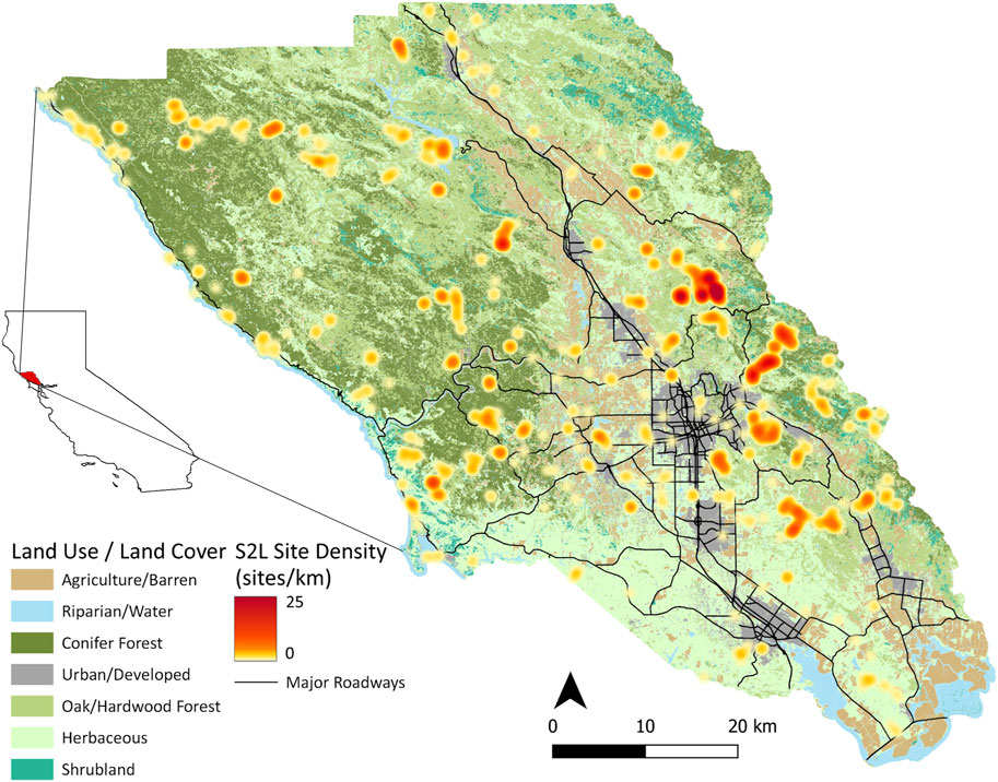
FIGURE 1. Sonoma County, California, United States land use/land cover classes from Sonoma County Fine-scale Vegetation and Habitat Map (sonomavegmap.org) used as a component of site selection stratification from 2017 to 2021 (n = 1,195).

TABLE 1

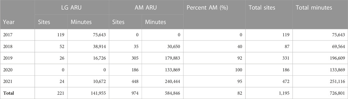
TABLE 1. Summary of acoustic sampling by year and device.

2.2 Acoustic features

2.2.1 Acoustic indices

We calculated 15 acoustic indices for each 1-min recording (Table 2 and Supplementary Material S1). We chose these indices because they have been frequently applied in terrestrial ecoacoustic and bioacoustic research (Sueur et al., 2014) and have consistently demonstrated varying sensitivity to sources of biophony, geophony, and anthropophony. We used minute-level values of indices to calculate two mean site-level values used in statistical analyses, one for 24-h and a second for morning only (4 a.m.–12 p.m.; used in bird species richness analyses).

TABLE 2

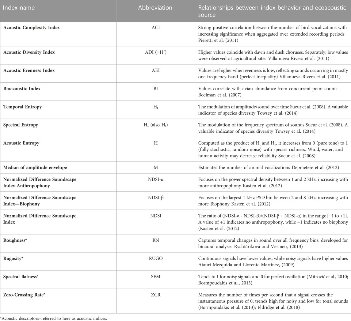
TABLE 2. Fifteen acoustic indices and descriptors for soundscape analysis from ecoacoustic studies.

2.2.2 Soundscape components

We used the percent presence of ABGQI soundscape events to investigate how sonic conditions in a large acoustic dataset relate to ecological indicators. We detected ABGQI events in our recordings using a convolutional neural network (CNN) classifier initially developed by and full details can be found in Quinn et al. (2022). Briefly, we generated probabilities for each ABGQI class for 21,804,030 2-s (2-s) samples (the CNN produces an independent probability for each class for each 2-s sample). The ABGQI probabilities were classified as present or absent using optimized class wise threshold values. The 2-s presences for each ABGQI class were then averaged for each site, resulting in a feature value for each soundscape component ranging from 0% to 100% present at the site-level. Two site-averages were calculated, one for 24-h and a second for morning only (4 a.m.–12 p.m.; used in bird species richness analyses). For example, if a site had 1,200 2-s samples from 40 1-min recordings, and anthropophony was predicted present in 300 of these 2-s samples, then 25% of recordings would be predicted to contain anthropophony. Notably, our ABGQI CNN treats each soundscape component independently, so any combination of soundscape components can be predicted for a given 2-s sample and will not necessarily sum to 100%. We interpret the effects of soundscape components as follows.

- Biophony: reflects general vocalizing animal activity. These primarily include bird calls and frog and insect choruses while capturing flying insect activity more uncommonly.

- Anthropophony: primarily reflects anthropogenic activity such as vehicle traffic, various combustion engines, and airplane activity.

- Quiet: reflects the general absence of emergent sound. We classified quiet to explicitly model periods of silence and not assume the absence of other soundscape components implied silence, as the CNN model included classification error of ABGI. A positive effect implies a relationship with more quiet periods, while a negative effect implies stronger effects from other soundscape components.

- Geophony: primarily reflects wind, as Sonoma County recordings show increased wind levels in the late afternoon (Quinn et al., 2022), and is considered non-ecologically meaningful ambient sound.

- Interference: reflects broad-frequency, rapid spikes in acoustic activity related to physical interferences with the ARU (e.g., branches hitting the ARU) or internal electronic malfunctions and is influenced by internal ARU self-noise. Interference results in higher acoustic activity that may be associated with events such as gusty winds, and we interpreted this as non-meaningful noise in recordings regardless of the cause of the interference event.

2.2.3 Acoustically-derived bird species richness

We used acoustically-derived bird species richness to measure biodiversity, which we then related to acoustic indices and soundscape components. The S2L project developed a separate CNN-based classification approach to identify 54 of the most common vocalizing bird species across Sonoma County (Clark et al., 2023). We derived bird species classification from three CNNs at 2-s intervals. For each bird species, we used the highest accuracy CNN to calculate the presence and absence of the species in all recordings and applied a lower cutoff of n = 3 positive classifications per site to indicate a presence for a given site, resulting in 1,185 sites with bird observations. We then summed all species detections at each site to arrive at site-level species richness for 24 h of recording and a “morning-only” subset targeting high bird activity periods (4 a.m.–12 p.m.). For both summaries, all 54 bird species had presences across sites, with the minimum richness of zero species for both datasets and the highest richness of 51 species (µ = 27.1 ± 7.3) for 24-h and 48 species (µ = 21.7 ± 6.7) for morning-only data, respectively.

2.3 Statistical analyses

2.3.1 Generalized additive modeling

We used generalized additive models (GAMs) to relate soundscape components and acoustic indices with one another and with bird species richness. GAMs are an even more flexible modeling option than generalized linear models, which provide benefits over ordinary linear models, such as allowing for non-normal error distributions and non-linear model structures (Wood, 2017).

All GAMs were fit using the R (R Core Team, 2022) package “mgcv” (Wood, 2017) using backward variable selection from full models. We generated partial dependence plots (PDPs) in R using the draw function from the “gratia” package (Simpson, 2022). We interpreted PDP slopes as the magnitude of influence a covariate had on the response, where higher absolute slope values were more influential for those areas in the covariate’s domain. Comparatively, a covariate with a near-zero slope had minimal effect on the response when included. For our final GAMs, we reported error distribution, link function, adj-R², and deviance, where applicable. We report deviance because it can better approximate non-normal error distributions for GAMs; however, deviance and adj-R² are equivalent for GAMs with a Gaussian error distribution. See Supplementary Material S2 for the full GAM fitting procedure.

2.3.2 Acoustic index sound composition

We investigated how soundscape components vary with each acoustic index using GAMs. All models were nested versions of the full model:

$\begin{array}{c}E\left({AcousticIndex}_i\right)={ARU}_i+\mathit{log}\left({Minutesrecorded}_i\right)\\ +f_1\left({Anthropophony}_i\right)+f_2\left({Biophony}_i\right)\\ +f_3\left({Geophony}_i\right)+f_4\left({Quiet}_i\right)\\ +f_5\left({Interference}_i\right)\end{array}(1)$

where for each site observation i, $f_j$ represents smooth functions for soundscape components, ARU has two levels (AM and LG, not individual device), and Minutes recorded_i is the logarithm of the number of 1-min recordings. We scaled soundscape component covariates using a min-max normalization. We used PDPs and slope summaries from soundscape component models to interpret significant model covariates for each acoustic index. Because GAMs had splines fit with up to k = 5 basis functions, a partial effect could have positive and negative effects throughout the covariate domain. Positive effects implied a covariate resulted in increases in the response, while negative effects implied an inverse relationship.

2.3.3 Case study: accounting for interference

GAM analyses indicate that the presence of ABGQI CNN-classified interference heavily influenced the ACI; thus, we performed an experiment to account for this effect. We removed any 1-min recording containing an interference sample and recalculated the average site soundscape components and ACI values. Removing recordings with interference reduced the dataset to 300,572 recordings (41.4% of data) and reduced sites to 1,194, though the average minutes per site were reduced from 608 ± 317 min to 251 ± 186 min, resulting in the rate of soundscape components changing (Table 3). We followed the same procedure to model ACI with GAMs as found in the “Generalized additive modeling” section. The resulting final model reflects the relationship between soundscape components and ACI without the effect of interference.

TABLE 3

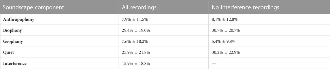
TABLE 3. The change in the rate of soundscape components after removing 1-min recordings with interference (mean and standard deviation).

2.3.4 Relationship between acoustic features and bird species diversity

We explored how soundscape components were associated with site-level bird species richness. First, we constructed a GAM to see how variance in biophony could be explained by bird species richness (Eq. 2):

$E\left({Biophony}_i\right)={ARU}_i+\mathit{log}\left({Minutesrecorded}_i\right)+f_1\left({Richness}_i\right)(2)$

where Richness_i is each site’s acoustically-derived bird species richness. We then designed three models to compare the ability of biophony and acoustic indices to predict bird species richness and reflect their joint ability to function as biodiversity indicators. First, biophony was used alone to model bird richness (Eq. 3):

$E\left({Richness}_i\right)={ARU}_i+\mathit{log}\left({Minutesrecorded}_i\right)+f_1\left({Biophony}_i\right)(3)$

Recent research suggests multiple acoustic indices can better represent diversity measures like avian vocal diversity (Buxton et al., 2018a; Allen-ankins et al., 2023) and be used to aid soundscape labeling of birds, insects, and geophony (Scarpelli et al., 2021) when used together. Therefore, we developed a GAM to relate all 15 acoustic indices to bird species richness to investigate 1) which acoustic indices best capture variation in richness and 2) the directional effect of significant acoustic indices (Eq. 4):

$\begin{array}{ll}\hfill E\left({Richness}_i\right)& ={ARU}_i+\mathit{log}\left({Minutesrecorded}_i\right)+f_1\left({ACI}_i\right)+f_2\left({ADI}_i\right)+f_3\left({AEI}_i\right)+f_4\left({BI}_i\right)+f_5\left(H_i\right)+f_6\left(H_{s_i}\right)+f_7\left(H_{t_i}\right)\hfill \\ \hfill & +f_8\left(M_i\right)+f_9\left({NDSI}_i\right)+f_{10}\left({NDSI-\alpha }_i\right)+f_{11}\left({NDSI-\beta }_i\right)+f_{12}\left(R_i\right)+f_{13}\left({Rugosity}_i\right)+f_{14}\left({SFM}_i\right)+f_{15}\left({ZCR}_i\right)\hfill \end{array}(4)$

Our third GAM combined biophony and all acoustic indices to assess the ability of all acoustic indicators to model bird species richness (Eq. 5):

$\begin{array}{l}\hfill E\left({Richness}_i\right)={ARU}_i+\mathit{log}\left({Minutesrecorded}_i\right)+f_1\left({ACI}_i\right)\\ +f_2\left({ADI}_i\right)+f_3\left({AEI}_i\right)+f_4\left({BI}_i\right)+f_5\left(H_i\right)\\ +f_6\left(H_{s_i}\right)+f_7\left(H_{t_i}\right)+f_8\left(M_i\right)+f_9\left({NDSI}_i\right)\\ +f_{10}\left({NDSI-\alpha }_i\right)+f_{11}\left({NDSI-\beta }_i\right)+f_{12}\left(R_i\right)\\ +f_{13}\left({Rugosity}_i\right)+f_{14}\left({SFM}_i\right)+f_{15}\left({ZCR}_i\right)\\ +f_{16}\left({Biophony}_i\right)\end{array}(5)$

We compared all model performances and variable selection for the morning-only and 24-h data to investigate whether targeting periods when bird species are more active results in a stronger relationship between acoustic features and bird species richness. We followed the approach outlined in the “Generalized additive modeling” section for all bird species richness models.

3 Results

3.1 Effects of soundscape components on acoustic indices

We modeled acoustic indices using soundscape components (Eq. 1), with model mean and standard deviation deviance explained of 66.8% ± 13.9% (Table 4). Because of the relatively large sample size (n = 1,195 sites), covariate significance levels were frequently highly significant (p < 0.05) when soundscape components were retained in the final GAMs (Supplementary Materials S3, S4). All final GAMs contain biophony, interference, and the ARU fixed effect. However, no model contains the number of recordings. The fitted model for BI is the only model not to include anthropophony, quiet is not in the final model for ACI, and geophony is not included in NDSI-α, NDSI, SFM, and RN (all abbreviations defined in Table 2).

TABLE 4

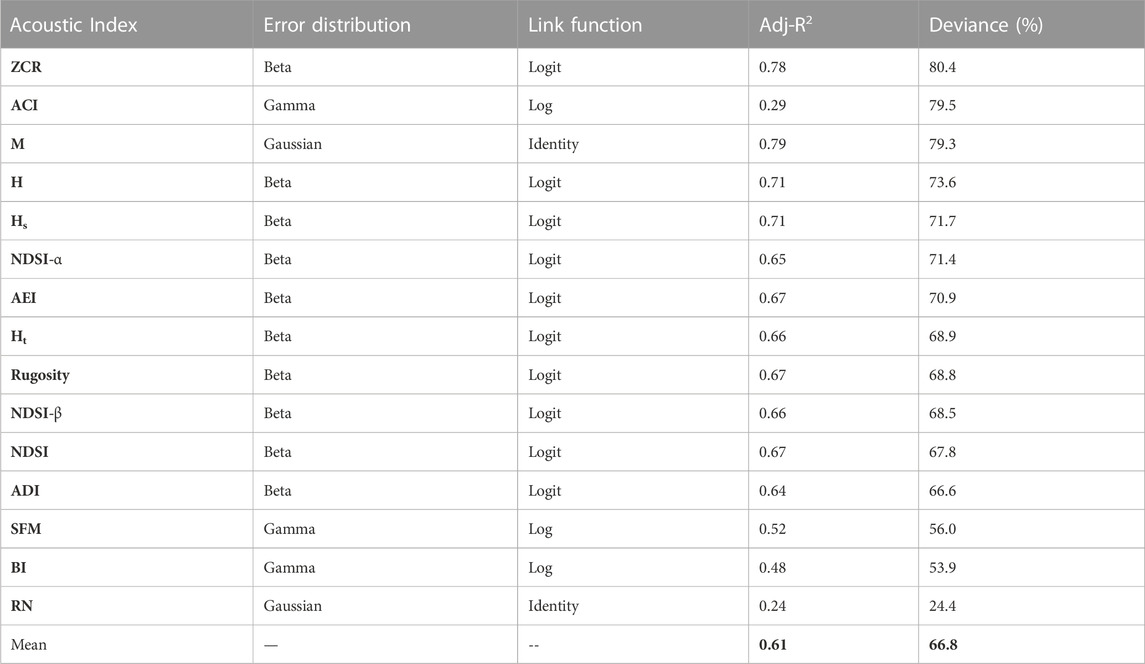
TABLE 4. Final GAM results and model structure, sorted by high to low deviance. Acoustic index abbreviations can be found in Table 2.

Figure 2 shows the influence on index values from the partial dependence on each sound component individually. Interference influences ACI most intensely based on all soundscape components’ high positive slope values. Furthermore, all sounds positively affect the value of ACI, and quiet is not included in the final model. Comparatively, RN is weakly influenced by interference, with values clustered around a slope of zero, while anthropophony and biophony have more significant, generally positive effects on RN.

FIGURE 2

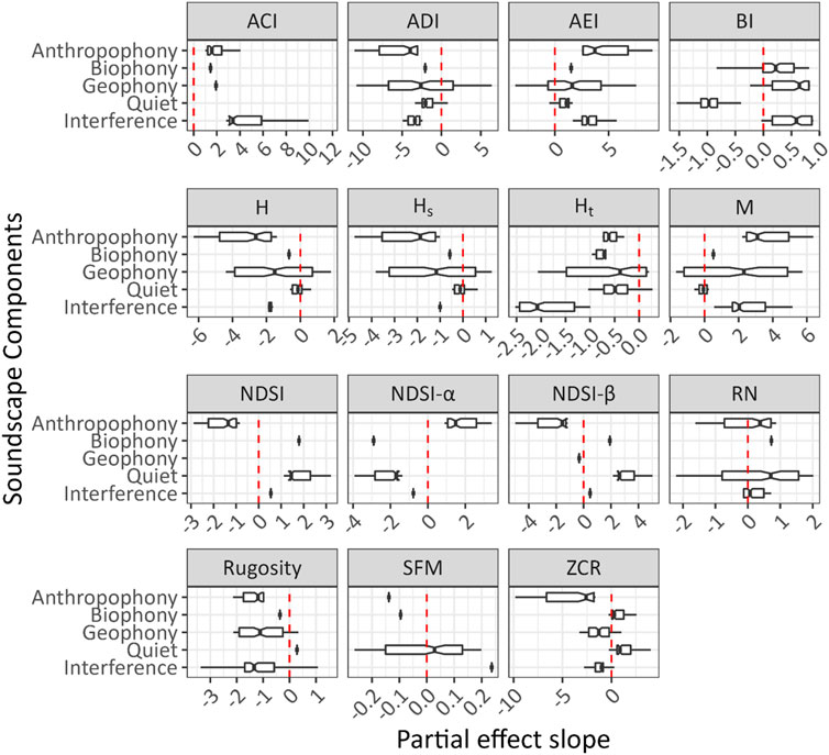
FIGURE 2. The effect of each sound component on index values in the GAM for each acoustic index, evaluated using the partial dependence of each sound component’s inner 99% range of values while holding all other components to their mean value. PDPs (Supplementary Material S4) show the index’s sensitivity to the sound component. Because these values are obtained for each component while holding the others constant, the total variance in index values for the sound component is highlighted. Higher variance in an index’s partial effect slope reflects higher sensitivity to the sound component. Values of x = 0 denote a zero slope in the PDPs and do not imply non-significance.

3.2 Case study: accounting for ambient sounds

After removing 1-min recordings with interference, we found biophony changed from being one of the least influential covariates modeling ACI to being the most influential soundscape component (Figure 3). Further, ACI became more robust to anthropophony, as indicated by lower slope values (Figure 4). Geophony’s effect is less linear and slightly more influential, although higher slope values occur primarily in geophony’s sparse higher values. Geophony’s effect on ACI may have increased because it is tightly linked to non-internal ARU interference events (e.g., wind co-occurring with interference), and when these events were removed, other geophony types (e.g., rain and running water) could explain more variation in ACI. After removing interference, GAM deviance decreased slightly from 79.5% to 74.4%. Quiet is included in the final GAM, although it was non-significant (p = 0.12).

FIGURE 3

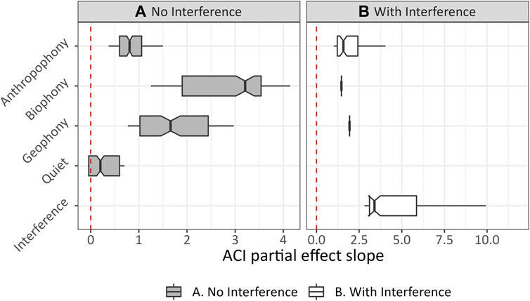
FIGURE 3. ACI GAM PDP slope summaries modeled recordings (A) without and (B) with interference, respectively.

FIGURE 4

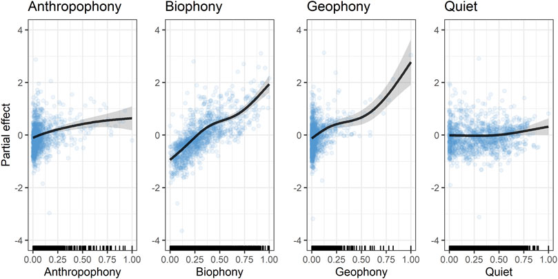
FIGURE 4. Cubic spline (black line) of PDPs of ACI modeled without interference. The y-axis shows the mean model ACI values (centered on zero), and the x-axis shows covariate values with ticks reflecting the density of observations. Changes across a covariate’s domain reflect its influence on ACI value. Shaded regions reflect 95% credible intervals of the spline, and blue points indicate partial residuals. Note that geophony values >0.5 are sparse yet heavily affect the behavior and precision of the spline.

3.3 Relationships of acoustic indices and biophony with bird species richness

The GAM modeling biophony as a function of bird species richness (Eq. 2) had 40.3% deviance explained (i.e., a measure of model fit), 12.9% RMSE, and included both ARU and the log number of recordings for the 24-h data. The morning-only model had higher performance (deviance = 45.4%) but higher error (RMSE = 15.3%). Both datasets show a strong positive relationship between bird species richness and biophony across all species richness values. Model fits capture the mean trend in bird species richness related to biophony but underestimate the variance at intermediate species richness values (e.g., 15–35 species).

We found the highest performing GAM modeling bird species richness (according to the greatest explained deviance) was the combined acoustic indices and biophony GAM using the morning-only dataset (Table 5). This model resulted in the highest deviance (65.8%; RMSE = 3.9 species; Figure 5), 2% higher than the 24-h model. In general, the morning-only GAMs, regardless of covariates, performed better than the 24-h GAMs. Most notably, there was a 6.8% better performance for the morning-only biophony GAM (Eq. (3)) than the 24-h GAM.

TABLE 5

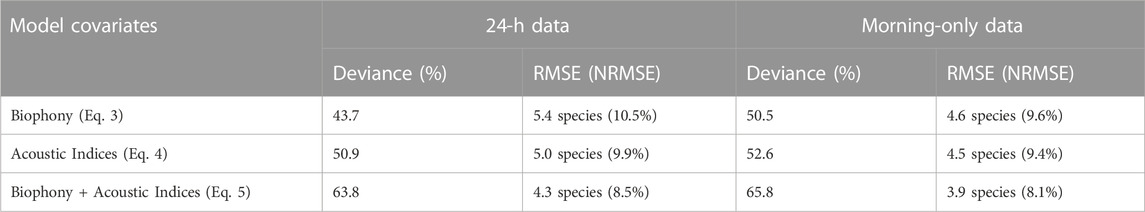
TABLE 5. Performance of bird species richness models with covariates of biophony (Eq. 3), acoustic indices (Eq. 4), and combined biophony and acoustic indices (Eq. 5), respectively. Normalized RMSE (NRMSE) was calculated using RMSE divided by species richness range (48 for morning-only and 51 for 24-h datasets).

FIGURE 5

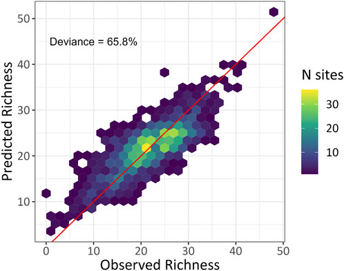
FIGURE 5. Predicted and observed bird species richness from the combined morning-only acoustic index and biophony GAM with the log number of recordings as a fixed effect. The density of sites is shown for observed and predicted values, and the red line indicates the 1:1 fit line.

The highest performing, morning-only GAM includes the log number of recordings along with biophony, ADI, AEI, BI, H, M, NDSI, NDSI-α, NDSI-β, RN, and ZCR (PDP in Supplementary Material S6). The number of recordings has a positive effect on bird species richness. Biophony, NDSI-β, and AEI have the largest effects of the included covariates, while ADI, BI, and RN have the smallest effects on bird species richness. AEI, BI, NDSI-β, and ZCR have concave-down shaped PDPs, but BI decreases across its entire domain. Biophony also has a concave-down PDP with the strongest positive effect from 0%–25%. NDSI-α has a concave up trend, while RN has a concave down to concave up trend across its domain, approximating a flattened sinusoid. H and M have negative linear effects, while ADI and RN have roughly linear, positive effects. Notably, NDSI has an unreliable PDP interpretation due to high concurvity and covariance structure with NDSI-α and NDSI-β. The 24-h model contained all covariates in the morning-only model in addition to ACI (Eq. 5).

4 Discussion

4.1 Contribution of soundscapes components to acoustic indices

All GAMs from Eq. 1 contained ARU effects suggesting systematic differences between ARU models. We believe this is most likely due to the hardware specification differences in the LG ARUS compared to the AM ARUs (see methods) where AM ARUs were more sensitive to distant sounds (Campos-Cerqueira and Aide, 2016) and highlights the need to include ARU type when considering sonic conditions (Haupert et al., 2022). Additionally, no acoustic index final models included the number of recordings. In our analyses, the amount of data collected did not strongly modulate the relationships between soundscape components and acoustic indices. However, Bradfer-Lawrence et al. (2019) recommend continuously sampling 120 h of data per site, or 26 weeks with the 1-min-in-10 as used here, to achieve stability in acoustic indicator variance, while our mean recording duration per site equated to 99 h of deployed recording time or 9.9 cumulative hours of recordings. We did not record for a sufficient duration to observe decreased variance at 120 h of recording, as in Bradfer-Lawrence et al. (2019), which may lead to this disparity in findings.

We found that biophony positively influenced NDSI-β, NDSI, AEI, BI, RN, ZCR, and ACI. This suggests these indices are related to vocalizing animals as these sounds were encompassed in the biophony CNN training and therefore possess ecologically-meaningful information about animal activity and diversity. Similarly, indices with greater influence from anthropophony and quiet could provide information related to anthropogenic impact on ecosystems and areas with quiet landscapes (Pavan, 2017), which in some cases could indicate ecosystem decline if there were previously high levels of biophony (Quinn et al., 2022). Indices strongly affected by geophony and interference (ACI, AEI, M, Rugosity, H, H_t, and ADI) should be used and interpreted judiciously because their outcomes may be more of a reflection of ambient noise than the ecology of the study domain.

Our findings corroborate some studies on soundscape components and acoustic indices yet contradict others. For example, Bradfer-Lawrence et al. (2019) found that high amounts of anthropophony and geophony led to high ADI values, while we found the inverse for anthropophony and a more complex but generally inverse relationship with geophony in our data, which aligns more with findings from Fairbrass et al. (2017). Patterns for H were consistent with prior work, namely, that anthropophony, geophony, and interference influence H to a larger degree than biophony; however, this contrasts with Ross et al. (2021), where H was relatively insensitive to confounding soundscape influences. Sueur et al. (2008) recommend a low-pass frequency filter of <200 Hz to reduce anthropophony and geophony effects; however, this recommendation would be minimally effective in our data because anthropophony events affected soundscapes up to 5,000 Hz (Quinn et al., 2022 Supplementary Material). The low-pass frequency filter would be adequate for most sources of geophony in our dataset. Other work has demonstrated ACI to be robust against rain events and NDSI as highly sensitive to rainfall (Sánchez-Giraldo et al., 2020). Here, we contribute to these findings and demonstrate ACI’s significant relationship to wind-related geophony, consistent with Depraetere et al. (2012) and NDSI’s lack of a significant relationship with wind events. Overall, many of our findings relating indices to observed richness agree with findings in other studies (e.g., ACI, BI, H, and M in Bradfer-Lawrence et al., 2019). However, we provide evidence that the anthropogenic (NDSI-α) and biotic (NDSI-β) components of NDSI have strong positive relationships with anthropophony and biophony, respectively, and may be more informative as separate indices than NDSI, which integrates both components. This finding corroborates prior results that demonstrate NDSI and the biotic component of NDSI are insensitive to confounding sonic conditions (Ross et al., 2021).

We also found that removing unwanted noise from interference events resulted in a more reliable application of ACI, as recommended in prior work (Fairbrass et al., 2017). This result supports the hypothesis that acoustic indices such as ACI may be generalizable across spatial and temporal domains and therefore measure universally meaningful aspects of the soundscape, so long as extraneous biasing sounds are accounted for beforehand. This is particularly important for the AM ARUs which recorded significantly more interference events than LG ARUs and could result in erroneous interpretation of interference as biophony. Even though biophony accounted for more variance in ACI than other soundscape components when removing interference, the level of data loss here may not be an ideal solution to improve index reliability for other recording archives. To avoid this data loss, the application of ACI would be most effective in sonically consistent environments using ARUs that are not prone to rapid, broad-frequency interference events. Recording schedules could also be designed to account for data loss to achieve desired total samples after the removal of interference. Previous studies have recommended accounting for low-amplitude sound pulses when applying ACI (Farina et al., 2016), though these methods do not appear to scale to our broad-frequency interference events. We believe source separation techniques will provide better options for events such as interference while minimizing data loss (Lin and Tsao, 2020) or future statistical analysis of the interaction between interference and other soundscape components.

Indices strongly affected by multiple soundscape components are more difficult to interpret in complex landscapes that contain multiple sonic conditions across numerous land-use and land-cover types like Sonoma County, while indices affected to a lesser extent by soundscape components are more straightforward to interpret (i.e., NDSI, R, and BI). Indicators strongly influenced by biophony and robust to the other soundscape components may be applied more broadly (NDSI and NDSI-β) than indices where biophony does not have as much influence (H, H_s, M). Depending on the acoustic index, anthropophony may be a meaningful category (e.g., NDSI-α) or a non-meaningful source of noise (e.g., ACI). We summarized the trends of acoustic indices with soundscape components (Table 6), and we recommend that future ecoacoustic work apply appropriate indices given a study’s sonic characteristics and desired acoustic target (e.g., sound pollution or biotic events).

TABLE 6

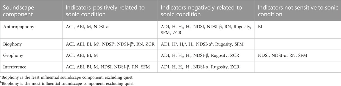
TABLE 6. When applying acoustic indices, consider the potential effects of soundscape components. We supply the dominant interpreted directional effects of the soundscape component on the index based on Figure 2 and PDPs in Supplementary Materials.

4.2 Predicting bird diversity with derived acoustic features

We sought to relate acoustic indices directly to species richness and followed recommendations to use indices in combination instead of independently (e.g., Buxton et al., 2018a; Bradfer-Lawrence et al., 2019). Our GAM approach with only acoustic indices (Eq. 4) resulted in comparable accuracy (adj-R² = 0.53; deviance/goodness of fit = 52.5%; n = 1,185) to another multi-index study that implemented Random Forest models to predict bird species vocalizations (R² = 0.40–0.51; Buxton et al., 2018a). Even though these findings were comparable, the ability of acoustic indices to represent bird species richness may be limited in acoustically-complex and heterogeneous environments (Buxton et al., 2018a) based on the effects of non-ecologically meaningful sounds on acoustic index patterns (Table 6). However, bird species richness models are not the only utility for multi-index models. Ensemble acoustic index modeling is promising when distinguishing degraded habitats from healthy habitats in marine settings (Williams et al., 2022) and terrestrial habitats (Bradfer-Lawrence et al., 2020) and monitoring vertebrate groups (Allen-ankins et al., 2023).

To extend the ability for acoustic indices to reflect biodiversity, we leveraged the automated detection of soundscape components to provide an empirical approach to predicting bird species diversity. The combined acoustic indices and biophony GAM (Eq. 5) slightly overpredicted at low species richness values and underpredicted at higher values (Figure 5). This pattern, particularly at higher richness values, may reflect the saturation and the inability of recordings to capture increases in species richness (Burivalova et al., 2019) or the model’s tendency to favor mean behavior over extreme values. However, the former explanation relates to sonic condition interactions, which result in the “masking” of unique signals. Notably, unlike anthropophony and geophony sources, animals are known to adjust their vocalization frequency and amplitude to increase propagation and success of signal reception (Pijanowski et al., 2011). Another consideration is that our detection data only included 54 species (a max richness of 48 in the morning data and 51 in the 24-h data), and a model with higher species richness values could resolve this potential saturation issue.

In the morning-only biophony and acoustic indices GAM, positive trends in biophony and NDSI-β support their utility as biodiversity indicators. Furthermore, reducing acoustic covariates from 16 to 11 suggests high redundancy in acoustic indices’ ability to explain variation in bird species richness. The negative trend in M aligns with other work showing that higher signal vocalizing activity leads to lower M values (Bradfer-Lawrence et al., 2019). However, this change from having a weak influence from biophony (Eq. 1) to a strong influence as a predictor of bird species richness demonstrates the need for caution when interpreting index effects.

In the 24-h dataset, acoustic indices were better predictors of bird species richness (Eq. 4) than biophony alone (Eq. 3). However, the performance for the morning-only biophony model (Eq. 3) had comparable performance to the acoustic index, 24-h GAM (Eq. 4). Our modeling is consistent with other work relating individual indices to bird richness and biophony (e.g., ADI: Machado et al., 2017; H_t, NDSI, ADI, AEI, M, ACI; Ross et al., 2021). Additionally, the ability for indices to better represent richness in a modeling framework over correlative analyses is consistent (Supplementary Material S7; Mammides et al., 2017). Overall, though, correlative relationships among indices and bird richness were weak here (|ρ| ≤ 0.35), and biophony had the strongest relationship (ρ = 0.56 for the morning only), reinforcing our emphasis on the utility of biophony as a more robust predictor of biodiversity metrics compared to acoustic indices. The ability of biophony to explain similar levels of species richness compared to 15 acoustic indices supports the utility of biophony as a viable ecoacoustic metric on par with combined acoustic indices and allows for targeted morning-only data collection. If biophony is unavailable, acoustic indices may provide higher performance and representation of bird species richness when using a 24-h sampling approach. Adding biophony to acoustic indices in an ensemble model (Eq. 5) increased the performance beyond comparable acoustic index models of bird diversity (Eq. 4; Buxton et al., 2018a).

4.3 Extension of biophony in ecoacoustics

Our analyses corroborate a finding from Fairbrass et al. (2017) and Ross et al. (2021) that acoustic indices applied in complex acoustic environments can reflect biotic activity, yet other sound sources significantly affect their replicability and make interpretation non-trivial. Namely, our analyses support NDSI-β as both relatively robust in varying sonic conditions (Ross et al., 2021) and the most representative index of bird species richness when biophony is unavailable. It is thus essential to understand assumptions and underlying effects of non-biotic sounds before interpreting index values (Gasc et al., 2015).

These analyses build on research that establishes that the cumulative amount of biophony, here quantified by our CNN, is a robust ecoacoustic indicator of biodiversity (Mullet et al., 2016; Fairbrass et al., 2019; Grinfeder et al., 2022). Compared to more traditional acoustic indices, biophony has the potential to be more directly related to animal diversity as it captures biotic events as opposed to an abstracted summary of acoustic energy as acoustic indices do, which at present can result in non-trivial relationships with underlying acoustic sources of sound. Furthermore, we believe CNN-derived metrics like biophony are potentially more robust to non-calibrated ARUs and methodological inconsistencies that influence acoustic index variation, but this issue requires formal study.

Our approach to quantifying biophony requires generalizability tests with other datasets and locations. Ideally, a future study would fine-tune the ABGQI CNN to reflect sounds in a different study domain. Even though this approach would require significant work to generate reference sound data, biophony as a general soundscape class is less intensive to generate from CNNs than those that detect species presences, which involve expert knowledge to identify reference species vocalizations (Clark et al., 2023). Non-experts can help in the effort to generate biophony reference data, as it does not involve species identification (Snyder et al., 2022). If not used as an ecoacoustic metric, biophony is valuable as a tool to aid researchers in filtering the ever-expanding size of acoustic datasets into relevant subsets for more efficient, targeted analyses (Pijanowski and Brown, 2022). In future efforts, periods with biophony may be broken into finer taxonomic granularity to understand specific family or species dynamics (Hao et al., 2022), expanding biophony’s value in conservation efforts (Dumyahn and Pijanowski, 2011).

With the rapidly advancing field of deep learning, CNN classification and source separation techniques (Lin and Tsao, 2020) may soon be more user-friendly to the point of competing with acoustic index calculations. Even if adapting our CNN or the development of a new CNN is outside a project’s scope, acoustic indices remain an approachable and relatively low-cost option for generating acoustic activity summaries, ensuring correct assumptions and a general understanding of how non-biotic noise influences values. Non-index quantification of soundscape dynamics using metrics like biophony may be more generalizable to measure changes in biodiversity and soundscapes incurring disturbance (e.g., increased anthropophony) and for targeted conservation and study (Grinfeder et al., 2022).

5 Conclusion

Our overarching goal was to understand how sonic conditions represented using soundscape components affect acoustic indices and improve interpretation. We applied a CNN classifier to detect soundscape components automatically, used statistical models to investigate their relationship with 15 common acoustic indices, and provided recommendations to contextualize the effects of soundscape components when applying these 15 acoustic indices. We found combining biophony and acoustic indices particularly informative for predicting bird species richness. We also validated how acoustic indices more reliably reflect biophony when non-biotic ambient noises are quantified and excluded from models. We aimed to provide a more flexible method to measure species richness acoustic activity than species-level identification in novel acoustic datasets. Our work supports applying more automated methods, such as CNN soundscape component detection, to acoustically assess and monitor biodiversity by establishing the combination of biophony and acoustic indices as useful ecoacoustic monitoring tools for bird species richness.

Data availability statement

Publicly available datasets were analyzed in this study. This data can be found here: sonomavegmap.org. The datasets generated for this study can be found alongside the associated code to reproduce results at github.com/CQuinn8/Ecoacoustic_indicators.

Author contributions

CQ: Conceptualization, Data curation, Formal analysis, Methodology, Software, Visualization, Writing—original draft. PB: Methodology, Writing–review and editing. CH: Methodology, Writing–review and editing. LS: Data curation, Funding acquisition, Methodology, Project administration, Writing–review and editing. BP: Writing–review and editing. SG: Funding acquisition, Resources, Supervision, Writing–review and editing. MC: Data curation, Conceptualization, Funding acquisition, Methodology, Resources, Supervision, Writing–review and editing. All authors contributed to the article and approved the submitted version.

Funding

The Soundscapes to Landscapes project was funded by NASA’s Citizen Science for Earth Systems Program (CSESP) under cooperative agreement 80NSSC18M0107.

Acknowledgments

We are grateful to the hundreds of citizen scientists who collected sound recordings and helped with bird CNN development in Soundscapes to Landscapes between 2017 and 2021. The following citizen scientists are recognized by name for their expert contributions of over 100 volunteer hours spent working on the project: Wendy Schackwitz, David Leland, Taylour Stephens, Jade Spector, Tiffany Erickson, Teresa Tuffli, Miles Tuffli, Katie Clas, and Bob Hasenick. We ran computational analyses on Northern Arizona University’s Monsoon computing cluster, funded by Arizona’s Technology and Research Initiative Fund. The Sonoma County land cover data used in our analyses was created with funding by NASA Grant NNX13AP69G, the University of Maryland, and the Sonoma Vegetation Mapping and LiDAR Program.

Conflict of interest

The authors declare that the research was conducted in the absence of any commercial or financial relationships that could be construed as a potential conflict of interest.

Publisher’s note

All claims expressed in this article are solely those of the authors and do not necessarily represent those of their affiliated organizations, or those of the publisher, the editors and the reviewers. Any product that may be evaluated in this article, or claim that may be made by its manufacturer, is not guaranteed or endorsed by the publisher.

Supplementary material

The Supplementary Material for this article can be found online at: https://www.frontiersin.org/articles/10.3389/frsen.2023.1156837/full#supplementary-material

References

Allen-ankins, S., Mcknight, D. T., Nordberg, E. J., Hoefer, S., Roe, P., Watson, D. M., et al. (2023). Effectiveness of acoustic indices as indicators of vertebrate biodiversity. Ecol. Indic. 147 (2022), 109937. doi:10.1016/j.ecolind.2023.109937

CrossRef Full Text | Google Scholar

Atauri Mezquida, D., and Llorente Martínez, J. (2009). Short communication. Platform for bee-hives monitoring based on sound analysis. A perpetual warehouse for swarm apos;s daily activity. Span. J. Agric. Res. 7 (4), 824. doi:10.5424/sjar/2009074-1109

CrossRef Full Text | Google Scholar

Boelman, N. T., Asner, G. P., Hart, P. J., and Martin, R. E. (2007). Multi-trophic invasion resistance in Hawaii: Bioacoustics, field surveys, and airborne remote sensing. Ecol. Appl. 17 (8), 2137–2144. doi:10.1890/07-0004.1

PubMed Abstract | CrossRef Full Text | Google Scholar

Bormpoudakis, D., Sueur, J., and Pantis, J. D. (2013). Spatial heterogeneity of ambient sound at the habitat type level: Ecological implications and applications. Landsc. Ecol. 28 (3), 495–506. doi:10.1007/s10980-013-9849-1

CrossRef Full Text | Google Scholar

Bradfer-Lawrence, T., Bunnefeld, N., Gardner, N., Willis, S. G., and Dent, D. H. (2020). Rapid assessment of avian species richness and abundance using acoustic indices. Ecol. Indic. 115, 106400. doi:10.1016/j.ecolind.2020.106400

CrossRef Full Text | Google Scholar

Bradfer-Lawrence, T., Gardner, N., Bunnefeld, L., Bunnefeld, N., Willis, S. G., and Dent, D. H. (2019). Guidelines for the use of acoustic indices in environmental research. Methods Ecol. Evol. 00, 1796–1807. doi:10.1111/2041-210X.13254

CrossRef Full Text | Google Scholar

Burivalova, Z., Game, E. T., and Butler, R. A. (2019). The sound of a tropical forest. Science 363 (6422), 28–29. doi:10.1126/science.aav1902

PubMed Abstract | CrossRef Full Text | Google Scholar

Buxton, R. T., Agnihotri, S., Robin, V. V., Goel, A., and Balakrishnan, R. (2018a). Acoustic indices as rapid indicators of avian diversity in different land-use types in an Indian biodiversity hotspot. J. Ecoacoustics 2, 1–17. doi:10.22261/jea.gwpzvd

CrossRef Full Text | Google Scholar

Buxton, R. T., McKenna, M. F., Clapp, M., Meyer, E., Stabenau, E., Angeloni, L. M., et al. (2018b). Efficacy of extracting indices from large-scale acoustic recordings to monitor biodiversity. Conserv. Biol., 32(5), 1174–1184. doi.org/doi:10.1111/cobi.13119

PubMed Abstract | CrossRef Full Text | Google Scholar

Campos-Cerqueira, M., and Aide, T. M. (2016). Improving distribution data of threatened species by combining acoustic monitoring and occupancy modelling. Methods Ecol. Evol. 7 (11), 1340–1348. doi:10.1111/2041-210X.12599

CrossRef Full Text | Google Scholar

Clark, M. L., Salas, L., Baligar, S., Quinn, C. A., Snyder, R. L., Leland, D., et al. (2023). The effect of soundscape composition on bird vocalization classification in a citizen science biodiversity monitoring project. Ecol. Inf. 75, 102065. doi:10.1016/j.ecoinf.2023.102065

CrossRef Full Text | Google Scholar

Depraetere, M., Pavoine, S., Jiguet, F., Gasc, A., Duvail, S., and Sueur, J. (2012). Monitoring animal diversity using acoustic indices: Implementation in a temperate woodland. Ecol. Indic. 13 (1), 46–54. doi:10.1016/j.ecolind.2011.05.006

CrossRef Full Text | Google Scholar

Dröge, S., Martin, D. A., Andriafanomezantsoa, R., Burivalova, Z., Fulgence, T. R., Osen, K., et al. (2021). Listening to a changing landscape: Acoustic indices reflect bird species richness and plot-scale vegetation structure across different land-use types in north-eastern Madagascar. Ecol. Indic. 120, 106929. doi:10.1016/j.ecolind.2020.106929

CrossRef Full Text | Google Scholar

Duarte, M. H. L., Sousa-Lima, R. S. S., Young, R. J., Vasconcelos, M. F., Bittencourt, E., Scarpelli, M. D. A., et al. (2021). Changes on soundscapes reveal impacts of wildfires in the fauna of a Brazilian savanna. Sci. Total Environ. 769, 144988. doi:10.1016/j.scitotenv.2021.144988

PubMed Abstract | CrossRef Full Text | Google Scholar

Dumyahn, S. L., and Pijanowski, B. C. (2011). Soundscape conservation. Landsc. Ecol. 26 (9), 1327–1344. doi:10.1007/s10980-011-9635-x

CrossRef Full Text | Google Scholar

Eldridge, A., Guyot, P., Moscoso, P., Johnston, A., Eyre-Walker, Y., and Peck, M. (2018). Sounding out ecoacoustic metrics: Avian species richness is predicted by acoustic indices in temperate but not tropical habitats. Ecol. Indic. 95, 939–952. doi:10.1016/j.ecolind.2018.06.012

CrossRef Full Text | Google Scholar

Fairbrass, A. J., Firman, M., Williams, C., Brostow, G. J., Titheridge, H., and Jones, K. E. (2019). CityNet—deep learning tools for urban ecoacoustic assessment. Methods Ecol. Evol. 10 (2), 186–197. doi:10.1111/2041-210X.13114

CrossRef Full Text | Google Scholar

Fairbrass, A. J., Rennett, P., Williams, C., Titheridge, H., and Jones, K. E. (2017). Biases of acoustic indices measuring biodiversity in urban areas. Ecol. Indic. 83, 169–177. doi:10.1016/j.ecolind.2017.07.064

CrossRef Full Text | Google Scholar

Farina, A., Pieretti, N., Salutari, P., Tognari, E., and Lombardi, A. (2016). The application of the acoustic complexity indices (ACI) to ecoacoustic event detection and identification (EEDI) modeling. Biosemiotics 9 (2), 227–246. doi:10.1007/s12304-016-9266-3

CrossRef Full Text | Google Scholar

Gasc, A., Pavoine, S., Lellouch, L., Grandcolas, P., and Sueur, J. (2015). Acoustic indices for biodiversity assessments: Analyses of bias based on simulated bird assemblages and recommendations for field surveys. Biol. Conserv. 191, 306–312. doi:10.1016/j.biocon.2015.06.018

CrossRef Full Text | Google Scholar

Gibb, R., Browning, E., Glover-Kapfer, P., and Jones, K. E. (2018). Emerging opportunities and challenges for passive acoustics in ecological assessment and monitoring. Methods Ecol. Evol. 2019, 169–185. doi:10.1111/2041-210X.13101

CrossRef Full Text | Google Scholar

Grinfeder, E., Haupert, S., Ducrettet, M., Barlet, J., Reynet, M. P., Sèbe, F., et al. (2022). Soundscape dynamics of a cold protected forest: Dominance of aircraft noise. Landsc. Ecol. 37 (2), 567–582. doi:10.1007/s10980-021-01360-1

PubMed Abstract | CrossRef Full Text | Google Scholar

Hao, Z., Zhan, H., Zhang, C., Pei, N., Sun, B., He, J., et al. (2022). Assessing the effect of human activities on biophony in urban forests using an automated acoustic scene classification model. Ecol. Indic. 144, 109437. doi:10.1016/j.ecolind.2022.109437

CrossRef Full Text | Google Scholar

Haupert, S., Sèbe, F., and Sueur, J. (2022). Physics-based model to predict the acoustic detection distance of terrestrial autonomous recording units over the diel cycle and across seasons: Insights from an Alpine and a Neotropical forest. Methods Ecol. Evol. 2023 (2022), 614–630. doi:10.1111/2041-210X.14020

CrossRef Full Text | Google Scholar

Hill, A. P., Prince, P., Piña Covarrubias, E., Doncaster, C. P., Snaddon, J. L., and Rogers, A. (2018). AudioMoth: Evaluation of a smart open acoustic device for monitoring biodiversity and the environment. Methods Ecol. Evol. 9 (5), 1199–1211. doi:10.1111/2041-210X.12955

CrossRef Full Text | Google Scholar

Kasten, E. P., Gage, S. H., Fox, J., and Joo, W. (2012). The remote environmental assessment laboratory’s acoustic library: An archive for studying soundscape ecology. Ecol. Inf. 12, 50–67. doi:10.1016/j.ecoinf.2012.08.001

CrossRef Full Text | Google Scholar

Krause, B. L. (2002). The loss of natural soundscapes. Earth Isl. J. 17, 27–29.

Google Scholar

Lin, T. H., and Tsao, Y. (2020). Source separation in ecoacoustics: A roadmap towards versatile soundscape information retrieval. Remote Sens. Ecol. Conservation 6 (3), 236–247. doi:10.1002/rse2.141

CrossRef Full Text | Google Scholar

Machado, R. B., Aguiar, L., and Jones, G. (2017). Do acoustic indices reflect the characteristics of bird communities in the savannas of Central Brazil? Landsc. Urban Plan. 162, 36–43. doi:10.1016/j.landurbplan.2017.01.014

CrossRef Full Text | Google Scholar

Magurran, A. E., Baillie, S. R., Buckland, S. T., Dick, J. M. P., Elston, D. A., Scott, E. M., et al. (2010). Long-term datasets in biodiversity research and monitoring: Assessing change in ecological communities through time. Trends Ecol. Evol. 25 (10), 574–582. doi:10.1016/j.tree.2010.06.016

PubMed Abstract | CrossRef Full Text | Google Scholar

Mammides, C., Goodale, E., Dayananda, S. K., Kang, L., and Chen, J. (2017). Do acoustic indices correlate with bird diversity? Insights from two biodiverse regions in yunnan province, south China. Ecol. Indic. 82, 470–477. doi:10.1016/j.ecolind.2017.07.017

CrossRef Full Text | Google Scholar

Mitrović, D., Zeppelzauer, M., and Breiteneder, C. (2010). Features for content-based audio retrieval. Adv. Comput. 78 (10), 71–150. doi:10.1016/S0065-2458(10)78003-7

CrossRef Full Text | Google Scholar

Moreno-Gómez, F. N., Bartheld, J., Silva-Escobar, A. A., Briones, R., Márquez, R., and Penna, M. (2019). Evaluating acoustic indices in the Valdivian rainforest, a biodiversity hotspot in South America. Ecol. Indic. 103, 1–8. doi:10.1016/j.ecolind.2019.03.024

CrossRef Full Text | Google Scholar

Mullet, T. C., Gage, S. H., Morton, J. M., and Huettmann, F. (2016). Temporal and spatial variation of a winter soundscape in south-central Alaska. Landsc. Ecol. 31 (5), 1117–1137. doi:10.1007/s10980-015-0323-0

CrossRef Full Text | Google Scholar

Pavan, G. (2017). “Fundamentals of soundscape conservation,” in Fundamentals of soundscape conservation (Wiley, Oxford, UK: Wiley-Blackwell), 235–258. doi:10.1002/9781119230724.ch14

CrossRef Full Text | Google Scholar

Pieretti, N., Farina, A., and Morri, D. (2011). A new methodology to infer the singing activity of an avian community: The Acoustic Complexity Index (ACI). Ecol. Indic. 11 (3), 868–873. doi:10.1016/j.ecolind.2010.11.005

CrossRef Full Text | Google Scholar

Pijanowski, B. C., and Brown, C. J. (2022). Grand challenges in acoustic remote sensing: Discoveries to support a better understanding of our changing planet. Front. Remote Sens. 2, 1–9. doi:10.3389/frsen.2021.824848

CrossRef Full Text | Google Scholar

Pijanowski, B. C., Farina, A., Gage, S. H., Dumyahn, S. L., and Krause, B. L. (2011). What is soundscape ecology? An introduction and overview of an emerging new science. Landsc. Ecol. 26 (9), 1213–1232. doi:10.1007/s10980-011-9600-8

CrossRef Full Text | Google Scholar

Quinn, C. A., Burns, P., Gill, G., Baligar, S., Snyder, R. L., Salas, L., et al. (2022). Soundscape classification with convolutional neural networks reveals temporal and geographic patterns in ecoacoustic data. Ecol. Indic. 138, 108831. doi:10.1016/j.ecolind.2022.108831

CrossRef Full Text | Google Scholar

R Core Team, (2022). R: A language and environment for statistical computing. R Foundation for Statistical Computing, Vienna, Austria. Available at: https://www.R-project.org/.

Google Scholar

Rappaport, D. I., Swain, A., Fagan, W. F., Dubayah, R., and Morton, D. C. (2022). Animal soundscapes reveal key markers of Amazon forest degradation from fire and logging. PNAS 119 (18), 21028781199–e2102878211. doi:10.1073/pnas.2102878119

CrossRef Full Text | Google Scholar

Retamosa Izaguirre, M. I., Ramírez-Alán, O., and De la O Castro, J. (2018). Acoustic indices applied to biodiversity monitoring in a Costa Rica dry tropical forest. J. Ecoacoustics 2, 1. doi:10.22261/jea.tnw2np

CrossRef Full Text | Google Scholar

Ross, S. R. P. J., Friedman, N. R., Yoshimura, M., Yoshida, T., Donohue, I., and Economo, E. P. (2021). Utility of acoustic indices for ecological monitoring in complex sonic environments. Ecol. Indic. 121, 107114. doi:10.1016/j.ecolind.2020.107114

CrossRef Full Text | Google Scholar

Rychtáriková, M., and Vermeir, G. (2013). Soundscape categorization on the basis of objective acoustical parameters. Appl. Acoust. 74 (2), 240–247. doi:10.1016/j.apacoust.2011.01.004

CrossRef Full Text | Google Scholar

Sánchez-Giraldo, C., Bedoya, C. L., Morán-Vásquez, R. A., Isaza, C. V., and Daza, J. M. (2020). Ecoacoustics in the rain: Understanding acoustic indices under the most common geophonic source in tropical rainforests. Remote Sens. Ecol. Conservation 6 (3), 248–261. doi:10.1002/rse2.162

CrossRef Full Text | Google Scholar

Scarpelli, M. D. A., Liquet, B., Tucker, D., Fuller, S., and Roe, P. (2021). Multi-index ecoacoustics analysis for terrestrial soundscapes: A new semi-automated approach using time-series motif discovery and random forest classification. Front. Ecol. Evol. 9, 1–14. doi:10.3389/fevo.2021.738537

CrossRef Full Text | Google Scholar

Simpson, G. L. (2022). gratia: Graceful ggplot-based graphics and other functions for GAMs fitted using mgcv. R package version 0.7.3.

Google Scholar

Snyder, R., Clark, M., Salas, L., Schackwitz, W., Leland, D., Stephens, T., et al. (2022). The soundscapes to landscapes project: Development of a bioacoustics-based monitoring workflow with multiple citizen scientist contributions. Citiz. Sci. Theory Pract. 7 (1), 24. doi:10.5334/cstp.391

CrossRef Full Text | Google Scholar

Sueur, J., and Farina, A. (2015). Ecoacoustics: The ecological investigation and interpretation of environmental sound. Biosemiotics 8 (3), 493–502. doi:10.1007/s12304-015-9248-x

CrossRef Full Text | Google Scholar

Sueur, J., Farina, A., Gasc, A., Pieretti, N., and Pavoine, S. (2014). Acoustic indices for biodiversity assessment and landscape investigation. Acta Acustica United Acustica 100 (4), 772–781. doi:10.3813/aaa.918757

CrossRef Full Text | Google Scholar

Sueur, J., Pavoine, S., Hamerlynck, O., and Duvail, S. (2008). Rapid acoustic survey for biodiversity appraisal. PLoS ONE 3 (12), 40655–e4110. doi:10.1371/journal.pone.0004065

PubMed Abstract | CrossRef Full Text | Google Scholar

Towsey, M., Wimmer, J., Williamson, I., and Roe, P. (2014). The use of acoustic indices to determine avian species richness in audio-recordings of the environment. Ecol. Inf. 21, 110–119. doi:10.1016/j.ecoinf.2013.11.007

CrossRef Full Text | Google Scholar

Villanueva-Rivera, L. J., Pijanowski, B. C., Doucette, J., and Pekin, B. (2011). A primer of acoustic analysis for landscape ecologists. Landsc. Ecol. 26 (9), 1233–1246. doi:10.1007/s10980-011-9636-9

CrossRef Full Text | Google Scholar

Williams, B., Lamont, T. A. C., Chapuis, L., Harding, H. R., May, E. B., Prasetya, M. E., et al. (2022). Enhancing automated analysis of marine soundscapes using ecoacoustic indices and machine learning. Ecol. Indic. 140, 108986. doi:10.1016/j.ecolind.2022.108986

CrossRef Full Text | Google Scholar

Wood, C. M., Popescu, V. D., Klinck, H., Keane, J. J., Gutiérrez, R. J., Sawyer, S. C., et al. (2019). Detecting small changes in populations at landscape scales: A bioacoustic site-occupancy framework. Ecol. Indic. 98, 492–507. doi:10.1016/j.ecolind.2018.11.018

CrossRef Full Text | Google Scholar

Wood, S. N. (2017). Generalized additive models: An introduction with R. 2nd edition. Boca Raton, FL: Taylor and Francis.

Google Scholar